High precision tests of QCD without scale or scheme ambiguities
The 40th anniversary of the
Brodsky–Lepage–Mackenzie method
Abstract
A key issue in making precise predictions in QCD is the uncertainty in setting the renormalization scale and thus determining the correct values of the QCD running coupling at each order in the perturbative expansion of a QCD observable. It has often been conventional to simply set the renormalization scale to the typical scale of the process and vary it in the range in order to estimate the theoretical error. This is the practice of Conventional Scale Setting (CSS). The resulting CSS prediction will however depend on the theorist’s choice of renormalization scheme and the resulting pQCD series will diverge factorially. It will also disagree with renormalization scale setting used in QED and electroweak theory thus precluding grand unification. A solution to the renormalization scale-setting problem is offered by the Principle of Maximum Conformality (PMC), which provides a systematic way to eliminate the renormalization scale-and-scheme dependence in perturbative calculations. The PMC method has rigorous theoretical foundations, it satisfies Renormalization Group Invariance (RGI) and preserves all self-consistency conditions derived from the renormalization group. The PMC cancels the renormalon growth, reduces to the Gell-Mann–Low scheme in the Abelian limit and leads to scale- and scheme-invariant results. The PMC has now been successfully applied to many high-energy processes. In this article we summarize recent developments and results in solving the renormalization scale and scheme ambiguities in perturbative QCD. In particular, we present a recently developed method the PMC∞ and its applications, comparing the results with CSS. The method preserves the property of renormalizable SU(N)/U(1) gauge theories defined as Intrinsic Conformality (iCF).
This property underlies the scale invariance of physical observables and leads to a remarkably efficient method to solve the conventional renormalization scale ambiguity at every order in pQCD.
This new method reflects the underlying conformal properties displayed by pQCD at NNLO, eliminates the scheme dependence of pQCD predictions and is consistent with the general properties of the PMC. A new method to identify conformal and -terms, which can be applied either to numerical or to theoretical calculations is also shown. We present results for the thrust and -parameter distributions in annihilation showing errors and comparison with the CSS. We also show results for a recent innovative comparison between the CSS and the PMC∞ applied to the thrust distribution investigating both the QCD conformal window and the QED limit. In order to determine the thrust distribution along the entire renormalization group flow from the highest energies to zero energy, we consider the number of flavors near the upper boundary of the conformal window. In this flavor-number regime the theory develops a perturbative infrared interacting fixed point. These results show that PMC∞ leads to higher precision and introduces new interesting features in the PMC. In fact, this method preserves with continuity the position of the peak, showing perfect agreement with the experimental data already at NNLO.
We also show a detailed comparison of the PMC∞ with the other PMC approaches: the multi-scale-setting approach (PMCm) and the single-scale-setting approach (PMCs) by comparing their predictions for three important fully integrated quantities , and up to the four-loop accuracy.
keywords:
QCD , Renormalization Group , Event Shape Variables , Higgs , Principle of Maximum Conformality1 Introduction
The renormalization scale and scheme ambiguities
The renormalization scale and scheme ambiguities are an important source of errors in many processes in perturbative QCD preventing precise theoretical predictions for both standard model (SM) and beyond standard model (BSM) physics. In principle, an infinite perturbative series is devoid of this issue, given the scheme and scale invariance of entire physical quantities [1, 2, 3, 4, 5]; in practice, perturbative corrections are known up to a certain order of accuracy and scale invariance is only approximated in truncated series, leading to scheme and scale ambiguities [6, 7, 8, 9, 10, 11, 12, 13, 14, 15, 16, 17, 18].
Although perturbative calculations for theoretical predictions are also affected by other sources of errors, e.g. the top- and Higgs-mass uncertainties and the strong-coupling uncertainty, the renormalization scale and scheme ambiguities remain among of the main sources of errors. These scale and scheme ambiguities play an important role for predictions in many fundamental processes in perturbative QCD, also with respect to the other sources of uncertainties. Processes such as gluon fusion in Higgs production [19] or bottom-quark production [20], which are essential for the physics investigated at the Large Hadron Collider (LHC) and at future colliders, are all affected by these ambiguities. In the present era, high-precision predictions are crucial for both SM and BSM physics, in order to test the theory in all sectors and to enhance sensitivity to possible new physics (NP) at colliders.
At the moment two basic strategies exist to deal with this problem. On one hand, according to conventional practice or conventional scale setting (CSS), this problem cannot be avoided and is responsible for part of the theoretical errors. The simple CSS procedure starts from the scale and scheme invariance of a given observable, which translates into complete freedom for the choice of renormalization scale. According to common practice, a first evaluation of the physical observable is obtained by calculating perturbative corrections in a given scheme (commonly used are or ) and at an initial renormalization scale . Thus, the renormalization scale is set to one of the typical scales of a process, , and errors are estimated by varying the scale over a range .
This method is claimed to evaluate uncalculated contributions from higher-order terms and that, due to the perturbative nature of the expansion, the introduction of higher-order corrections would reduce the scheme and scale ambiguities order by order. There is no doubt that the higher the order of the loop corrections calculated, the greater is the precision of the theoretical estimates in comparison with the experimental data, but we cannot determine a priori the level of accuracy necessary for the CSS to achieve the desired precision. And in the majority of cases at present only the NNLO corrections are available. Moreover, the divergent nature of the asymptotic perturbative series and the presence of factorially growing terms (i.e. renormalons [21, 22, 23] severely compromise the theoretical predictions.
However, even though this procedure may give an indication as to the level of conformality and convergence reached by the truncated expansion, it leads to a numerical evaluation of theoretical errors that is quite unsatisfactory and strongly dependent on the value of the chosen scale. Moreover, this method gives predictions with large theoretical uncertainties that are comparable with the calculated order correction; different choices of the renormalization scale may lead to very different results when higher-order corrections are included. For example, the NLO correction to jets with the BlackHat code [24] can range from negligible to extremely severe, depending on the choice of the particular renormalization scale. One may argue that the proper renormalization scale for a fixed-order prediction may be judged by comparing theoretical results with experimental data, but this method would be strongly process dependent and would compromise the predictivity of the pQCD approach.
Besides the complexity of the higher-order calculations and the slow convergence of the perturbative series, there are many critical points in the CSS method:
-
1.
In general, the proper renormalization scale value, , is not known, nor the correct range over which the scale and scheme parameters should be varied in order to obtain the correct error estimate. In fact, in some processes there can be more than one typical momentum scale that may be taken as the renormalization scale according to the CSS procedure; for example, in processes involving heavy quarks typical scales are either the center-of-mass energy or also the heavy-quark mass. Moreover, the idea of the typical momentum transfer as the renormalization scale only sets the order of magnitude of the scale, but does not indicate the optimal scale.
-
2.
No distinction is made among different sources of errors and their relative contributions; e.g. in addition to the errors due to scale-scheme uncertainties there are also errors from missing uncalculated higher-order terms. In such an approach theoretical uncertainties can become quite arbitrary and unreliable.
-
3.
The convergence of the perturbative series in QCD is affected by uncancelled large logarithms as well as by “renormalon” terms that diverge as at higher orders [21, 22]; this is known as the renormalon problem [23]. Such renormalon terms can give sizable contributions to the theoretical estimates, as shown in annihilation, decay, deeply inelastic scattering and hard processes involving heavy quarks. These terms are responsible for important corrections at higher orders also in the perturbative region, leading to different predictions according to the different choices of scale (as shown in Ref. [24]). Large logarithms on the other hand can be resummed using the resummation technique [25, 26, 27, 28, 29, 30, 31] and results are IR renormalon free. This does not help for the renormalization scale and scheme ambiguities, which still affect theoretical predictions with or without resummed large logarithms. In fact, as recently shown in Ref. [20] for the -production cross-section at NNLO-order accuracy at hadron colliders, the CSS scale setting leads to theoretical uncertainties that are of the same order as the NNLO corrections , taking as the typical momentum scale the -quark mass GeV.
-
4.
In the Abelian limit at fixed with , a QCD case effectively approaches the analogous QED case [32, 33]. Thus, to be self-consistent, any QCD scale-setting method should also be extendable to QED and results should be in agreement with the Gell-Mann–Low (GM–L) scheme. This is an important requirement also from the perspective of a grand unified theory (GUT), where only a single global method for setting the renormalization scale may be applied and then it can be considered as a good criterion for verifying if a scale setting is correct or not. CSS leads to incorrect results when applied to QED processes. In the GM–L scheme, the renormalization scale is set with no ambiguity to the virtuality of the exchanged photon/photons, which naturally sums an infinite set of vacuum polarization contributions into the running coupling. Thus, the CSS approach of varying the scale by a factor 2 is not applicable to QED, since the scale is already optimized.
-
5.
The large amount of forthcoming high-precision experimental data, produced especially by the running at high collision energy and high luminosity of the Large Hadronic Collider (LHC), will require more accurate and refined theoretical estimates. The CSS appears to be more a “guess”; its results are afflicted by large errors and the perturbative series converges poorly with or without large-logarithm resummation or renormalon contributions. Moreover, within such a framework, it is almost impossible to distinguish between SM and BSM signals and in many cases, improved higher-order calculations are not expected to be available in the short term.
To sum up, the conventional scale-setting method assigns an arbitrary range and an arbitrary systematic error to fixed-order perturbative calculations that greatly affects the predictions of pQCD. On the other hand, various strategies for optimization of the truncated expansion have been proposed. We point out that since its very beginning, several attempts have been performed to improve the renormalization procedure and different schemes have been introduced mainly to improve the convergence of the perturbative series. An example is the introduction of the , as suggested in Refs.[34, 35] and later the introduction of the momentum subtraction scheme (MOM) as discussed by Celmaster and Gonsalves in Refs. [36, 6]. The MS scheme, introduced in Ref. [37], is in fact quite arbitrary and related to the particular regularization scheme used, leading to a rather higher second-order contribution in the DIS process, by reabsorbing the scheme term into a redefinition of the QCD scale parameter , Bardeen et al. noticed a significant improvement of the convergence of the perturbative series. Later, the introduction of the MOM scheme, though being gauge dependent, has been shown to also include other scheme terms into , leading to a scheme which is less dependent on the regularization procedure and tending to a more "physical" scale and nearly to an "optimization procedure" [6]. A recent discussion on the gauge dependence of the MOM scheme has been given in Ref. [38]. We discuss these schemes in more detail in Sec. 2.3.
In general, an optimization or scale-setting procedure is considered reliable if it preserves important self-consistency requirements. All Renormalization Group properties, such as uniqueness, reflexivity, symmetry and transitivity should also be preserved by the scale-setting procedure in order to be generally applied [39]. A fundamental requirement is the scheme independence; other requirements can be suggested by known tested theories (such as QED), by the convergence behavior of the series in particular kinematic regions or by important phenomenological results.
The Principle of Minimal Sensitivity (PMS) is an optimization procedure proposed by Stevenson [11, 10, 9, 8] based on the assumption that, since observables should be independent of the particular RS and scale, their optimal perturbative approximations should be stable under small RS variations. The RS-scheme parameters and the scale parameter (or the subtraction point ) are considered “unphysical” and independent variables; their values are thus set in order to minimize the sensitivity of the estimate to their small variations. This is essentially the core of Optimized Perturbation Theory (OPT) [9], based on the PMS procedure. The convergence of the perturbative expansion is improved by requiring its independence from the choice of RS and . Optimization is implemented by identifying the RS-dependent parameters in the truncated series ( for and ), with the request that the partial derivative of the perturbative expansion of the observable with respect to the RS-dependent and scale parameters vanishes. In practice, the PMS scale setting is designed to eliminate the remaining renormalization and scheme dependence in the truncated expansions of the perturbative series.
We would argue that this approach is based more on convergence rather than physical criteria. In particular, the PMS is a procedure that can be extended to higher order and it can be generally applied to calculations obtained in arbitrary initial renormalization schemes. Although this procedure leads to results that are suggested to be unique and scheme independent, it unfortunately violates important properties of the renormalization group, as shown in Ref. [40], such as reflexivity, symmetry, transitivity and also the existence and uniqueness of the optimal PMS renormalization scheme are not guaranteed since they are strictly related to the presence of maxima and minima.
Another optimization procedure, namely the Fastest Apparent Convergence (FAC) criterion was introduced by Grunberg and is based on the idea of effective charges. As pointed out by Grunberg [12, 13, 14], any perturbatively calculable physical quantity can be used to define an effective coupling, or “effective charge”, by entirely incorporating the radiative corrections into its definition. Effective charges can be defined from an observable starting from the assumption that the infinite series of a given quantity is scheme and scale invariant. The effective charge satisfies the same renormalization group equations as the usual coupling. Thus, the running behavior for both the effective coupling and the usual coupling are the same if their RG equations are calculated in the same renormalization scheme. This idea has been discussed in more detail in Refs. [41, 42].
An important suggestion is that all effective couplings defined in the same scheme satisfy the same RG equations. While different schemes or effective couplings would lead to different renormalization group equations. Hence, any effective coupling can be used as a reference for the particular renormalization procedure. In general, this method can be applied to any observable calculated in any RS, also in processes with large higher-order corrections. The FAC scale setting, as has been shown in Ref. [40], preserves the RG self-consistency requirements, although the FAC method can be considered more an optimization approach rather than a proper scale-setting procedure to extend order by order. FAC results depend sensitively on the quantity to which the method is applied. In general, when the NLO correction is large, the FAC proves to be a resummation of the most important higher-order corrections and thus a RG-improved perturbation theory is achieved.
PMS and FAC are procedures commonly in use for scale setting in perturbative QCD together with CSS and an introduction to these methods can be found in Refs. [40, 43]. However, as shown in Refs. [44], these optimization methods not only have the same difficulties of CSS, but they also lead to incorrect and unphysical results in particular kinematic regions.
A solution to the renormalization scale setting problem is offered by the Principle of Maximum Conformality (PMC) [45, 46, 47, 48]. This method is the generalization and extension of the original Brodsky-Lepage-Mackenzie (BLM) method [15] to all theories, to all orders and to all observables and it satisfies all the theoretical requirements of a reliable scale-setting procedure at once, leading to accurate and consistent results. The primary purpose of the PMC method is to solve the scale-setting ambiguity; it has been extended to all orders [49, 50] and it determines the correct running coupling and the correct momentum flow according to RGE invariance [51, 52]. This leads to results that are invariant with respect to the initial renormalization scale and in agreement with the requirement of scale invariance of observables in pQCD [40]. The approach provides a systematic method to eliminate renormalization scheme and scale ambiguities from first principles by absorbing the terms, which govern the behavior of the running coupling via the renormalization group equation. Thus, the divergent renormalon terms cancel, improving convergence of the perturbative QCD series. Furthermore, the resulting PMC predictions do not depend on the particular scheme used, thereby preserving the principles of renormalization group invariance [39, 51]. The PMC procedure is also consistent with the standard Gell-Mann–Low method in the Abelian limit, [32]. Moreover, in a theory unifying all forces (electromagnetic, weak and strong interactions), such as Grand Unified Theories, one cannot trivially apply a different scale-setting or analytic procedure to different sectors of the theory. The PMC offers the possibility to apply the same method to all sectors of a theory, starting from first principles, eliminating renormalon growth, scheme dependence, scale ambiguity and satisfying the QED Gell-Mann–Low scheme in the zero-color limit .
PMC and schemes
We remark that the fundamental task of the PMC is to solve the renormalization scale and scheme ambiguities and in order to achieve this, it makes use of the RG-equations to reabsorb the -terms that are related to the UV-divergent diagrams. The procedure of the PMC works with any initial definition of the scheme or scale for the running coupling, MS or or the ’t Hooft scheme are all equivalent, since the entire scheme dependence of the observable is reabsorbed into the running coupling and into the PMC scale in the final series. In particular, the lower order terms, , of the -function are scheme independent; thus a scheme transformation cannot lead to a prescription for determining the scale. In fact, also in the case of the ’t Hooft scheme (as shown in Refs.[53, 54]) one can eliminate all scheme dependent coefficients, but there is no prescription for the renormalization scale, which can be considered as the first scheme parameter. Moreover, what seems a good prescription for the running coupling is not necessarily a good prescription for the entire fixed-order calculated quantity. In fact, still considering the ’t Hooft case, the entire series of is removed from the definition of the coupling, but in a fixed-order calculation these coefficients would have an impact on the coefficients of the series at each order of calculation and on the convergence of the series. On the other hand, the PMC gives a prescription for fixing the scale and reabsorbing all scheme-dependent terms of a cross-section into the running coupling and into the PMC scale, exposing the perturbative series to a minimization/cancellation of the effects of the scale and scheme uncertainties. An important consequence of the PMC procedure is the RS-invariance of the resulting series. We refer to RS-scheme invariance as the invariance under the extended-renormalization group and its equations (xRGE)[9, 55, 56, 17]. It can be shown that the PMC procedure may be performed either way using the same xRGE111We will discuss this procedure in detail in a future work soon.. The xRGE show that different scheme definitions can be related at the lowest order by a scale transformation for the case of the minimal subtraction schemes (MS and ) and the momentum space subtraction (MOM) scheme, but using the PMC, results would be scheme independent. A recent argument on the scheme dependence of the first conformal coefficient by Stevenson [57] is incorrect. The reason is that he assumes the coefficient of the scheme to be totally free with respect to the structure of the color factors and that it can be reabsorbed into the parameter. There are several reasons why this certainly leads to wrong results. First, two different couplings in two different schemes at NLO can only be related by a scale transformation according to the RG group, i.e. by a shift of the type: as shown also in Ref. [17]. In fact, given the scheme invariance of the , the only parameter that can be varied at NLO is the renormalization scale , which can have any real value or at most any value in the complex plane. Thus, the only scheme terms that can be reabsorbed into the scale (either the or the renormalization scale ) are those related to a shift of the scale using the standard RG group equations. This corresponds to the freedom of subtracting out any finite value together with the pole, in the renormalization procedure (e.g. MS and ). If one takes the freedom to vary the scheme according to any other relation that does not correspond to a "proper" RG equation at NLO, this consequently modifies the structure of the color factors for the coupling and thus would obtain a wrong result. If one follows this misleading assumption, one can obtain any result outside of a given initial theory and this is certainly not the aim of the xRGE, which should preserve the invariance of the final result. Moreover, if one changes the color structure for the coupling, one should be aware that, to be consistent, also the structure of the entire fixed-order calculation should be varied accordingly; though we do not agree with this procedure since a change of the color structure correspond to a change of the initial SU(N) theory (e.g. from QCD to QED Ref.[32]). Thus, any relation among couplings in different schemes, which can have perturbative validity in QCD but which cannot be considered as "proper" xRG transformations, should be considered as matching relations among quantities defined in different approximations or obtained using different approaches. Also in this case, results can be improved using the PMC and the residual dependence on the particular implicit definition of the "scheme" can be suppressed perturbatively by adding higher-order calculations. It can be shown that also in this case the results obtained are scheme-independent (e.g. see Ref. [58]). One may point out that, though the LO and the NLO conformal coefficient are scheme invariant, the higher-order conformal coefficients can be scheme dependent, we can answer that in the worst case this scheme dependence for any of the PMCs procedures is highly suppressed. Another argument in Ref. [57] by Stevenson, which is based on the principle of minimum sensitivity (PMS), we hold to be incorrect. Since the PMS is based on the assumption that all the unknown higher-order terms give zero contribution to the pQCD series [9], its prediction directly breaks the standard renormalization group invariance [39, 51], its pQCD series does not have normal perturbative features [59] and can be treated as an effective prediction only when we know the series up to high enough orders and the conventional series has already shown good perturbative features [60]. On the other hand, the PMC respects all features of the renormalization group, and its prediction satisfies all the requirements of standard renormalization group invariance [39, 51, 58, 52]. Moreover, given that the PMC preserves the RG invariance, it is possible to define CSR - Commensurate Scale Relations[50] among the effective charges relating observables in different "schemes" preserving all the group properties. Applying the PMC and the CSRs, one can relate effective couplings, as also conformal coefficients, leading to scheme-independent results for the observables. We remark that in order to apply the PMC correctly, one should be able to distinguish among the nature of the different -terms: whether they are related to the running of the coupling, to the running of masses or to UV-finite diagrams and in a deeper analysis also to the particular UV-divergent diagram (as discussed in Refs. [61, 48]). Once all -terms have been associated with the correct diagram or parameter, conformal coefficients are RG invariant and match the coefficients of a conformal theory. Applications of the PMC to different quantities (see Ref. [62, 63]) have recently shown a direct improvement of theoretical predictions. Moreover, a deeper insight into the QCD coupling at all scales, including , has been recently achieved (e.g. see Refs. [64, 65]), showing results consistent with the PMC.
PMC applications
So far, the PMC approach has been successfully applied to many high-energy processes, including Higgs boson production at the LHC [66], Higgs boson decays to [67, 68], and [69, 70, 71, 72, 73, 63] processes, top-quark pair production at the LHC and Tevatron [74, 47, 75, 76, 77, 78, 79], decay process [80, 81], semihard processes based on the BFKL approach [82, 83, 84], electron–positron annihilation to hadrons [49, 50, 51], hadronic boson decays [85, 86], the event shapes in electron–positron annihilation [87, 88, 89, 90, 91], the electroweak parameter [92, 93], leptonic decay [94, 95], and charmonium production [96, 97, 98] and decay [99, 100, 101, 102]. As shown in Ref. [103], by using the PMC, one can obtain a smooth transition for the running behavior between Bjorken sum rule effective coupling in the V-scheme and the Light-Front Holographic QCD (LFHQCD) coupling, going from the perturbative to the non nonperturbative domain respectively. In addition, the PMC provides a possible solution to the puzzle [104] and to the puzzle [105].
In particular, with regard to the PMC application to top-quark pair hadroproduction, the resulting production cross-sections agree with precise experimental data, and the large discrepancies of the top-quark forward-backward asymmetries between SM estimations and experimental measurements are greatly reduced [47, 74, 75, 76, 77]. Recently, an improved QCD prediction for the top-quark decay process obtained by using the PMC has also been presented in Ref.[80].
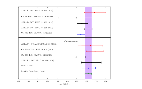
A precise top-quark mass can be extracted by the comparison of precise PMC predictions of production cross-sections with experimental data measured at LHC [78, 79]. The determined top-quark pole mass GeV, from the LHC measurement at TeV [79] agrees with the world average cited by the Particle Data Group (PDG) [106]. More explicitly, we present a summary of the top-quark pole masses in Fig.(1.1), where our PMC result and previous determinations from collider measurements at different energies and different techniques are presented. Owing to unknown higher-order contributions, this leads to two kinds of residual scale dependence for PMC predictions. However, these two residual scale dependencies are distinct from the conventional scale ambiguities, they are given by the unknown higher-order uncalculated contributions, while the scale dependence of the CSS is related more to the calculated orders. Thus, the residual scale dependence of the PMC results from the unknown higher-order terms and is an unavoidable intrinsic feature of the perturbative approach. It is to be noted that two of the three PMC ambiguities identified in Ref.[107] correspond exactly to two kinds of residual scale dependence. These two residual scale dependencies are highly suppressed; however, if the pQCD convergence of the perturbative series of either the PMC scale or the pQCD approximant is weak, such residual scale dependence could be significant. A recent discussion of the residual scale dependence of PMC predictions can also be found in the review [52].
Outline
In this review we display recent developments in solving the renormalization-scale and -scheme ambiguities based on the PMC and present some fundamental applications and results.
With respect to the previous reviews on the PMC (Refs. [40, 52]), in this review we focus on the recently developed method, namely the Infinite-Order Scale-Setting using the Principle of Maximum Conformality (PMC∞), showing first some of its applications and new features, and then a comparison of this method with the CSS and the other PMC approaches, such as the multi-scale (PMCm), and the single-scale PMC (PMCs), on the Event Shape Variables and on some crucial fully integrated quantities: , and .
More in detail: in Section I we give an introduction to the renormalization scale setting problem in QCD; in Section II we recall fundamental equations of the renormalization group and their extended version, starting from the renormalization procedure of the strong coupling and its renormalization scale dependence; in Section III we summarize formulas and basic concepts of the PMC approach with its features and methods (PMCm, PMCs); in Section IV we introduce the newly developed method PMC∞ and its new features; in Section V we show results for the application of the PMC∞ to the event-shape variables: thrust and -parameter, we show particularly new features of the PMC performing interesting limits for thrust (IR conformal and QED limit) and comparing the results under the CSS and the PMC∞ methods; in this section we also show a novel method to determine the strong coupling and its behavior over a wide range of scales, from a single experiment at a single scale, using the event-shape variable results; in Section VI we present a detailed comparison of the CSS, PMCs, PMCm and PMC∞ methods tested on fundamental fully integrated quantities at 4 loops: , and ; finally, in Section VII we summarize and discuss the results.
2 Renormalization Scale and Scheme invariance
The focus of this section is the strong coupling constant and its renormalization-scale and -scheme dependence. We summarize fundamental basic theoretical results and updated formulas regarding the renormalization group.
2.1 The Renormalization Group
QCD is a renormalizable theory, which means that the infinite number of ultraviolet (UV) singularities that arise in loop integration may be reabsorbed into a finite number of parameters entering the Lagrangian: the masses, coupling constant and fields.
The procedure starts from the assumption that the variables entering the Lagrangian are not the effective quantities measured in experiments, but are unknown functions affected by singularities. The origin of the ultraviolet singularities is often interpreted as a manifestation that a QFT is a low-energy effective theory of a more fundamental yet unknown theory. The use of regularization UV cut-offs shields the very short-distance domain, where the perturbative approach to QFT ceases to be valid.
Once the coupling has been renormalized to a measured value and at a given energy scale, the effective coupling is no longer sensitive to the ultraviolet (UV) cut-off, nor to any unknown phenomena arising beyond this scale. Thus, the scale dependence of the coupling can be well understood formally and phenomenologically. Actually, gauge theories are affected not only by UV, but also by infrared (IR) divergencies. The cancellation of the latter is guaranteed by the Kinoshita-Lee-Nauenberg (KLN) theorem [108, 109].
Considering first the Lagrangian of a massless theory, which is free of any particular scale parameter, in order to deal with these divergences a regularization procedure is introduced. Referring to the dimensional regularization procedure [37, 110, 111], one varies the dimension of the loop integration, and introduces a scale in order to restore the correct dimension of the coupling.
In order to determine the renormalized gauge coupling, we consider the quark-quark-gluon vertex and its loop corrections. UV-divergences arise from loop integration for higher-order contributions for both the external fields and the vertex. The renormalization constants of the vertices are related by Slavnov-Taylor identities, in particular:
| (2.1) |
where is the coupling renormalization constant, is the vertex renormalization constant, and are:
the renormalization constants for gluon and quark fields respectively. The superscript indicates renormalized fields. The renormalization constants in dimensional regularization are given by:
| (2.2) | |||||
| (2.3) | |||||
| (2.4) |
where is the regulator parameter for the UV-ultraviolet singularities. We have labelled the number of flavors related to the UV singular diagrams.222Throughout the paper we use the following notation: for the general number of active flavors, to indicate the number of flavors related to the UV-divergent and for the UV-finite diagrams. By substitution, we have that the UV divergence:
| (2.5) |
with
| (2.6) |
The singularities related to the UV poles are subtracted out by a redefinition of the coupling. In the scheme, the renormalized strong coupling is related to the bare coupling by:
| (2.7) |
In the minimal subtraction scheme () only the pole related to the UV singularity is subtracted out. A more suitable scheme is [35, 112, 113], where the constant term is also subtracted out. Different schemes can also be related by scale redefinition, e.g. . We remark that the renormalization procedure leads to a unique renormalization constant for the strong coupling. In fact, the other renormalization constants, such as , , i.e. the renormalization constants for 3-gluon, 4-gluon, ghost-ghost-gluon, quark-quark-gluon vertex respectively, are related to it via the Slavnov–Taylor identities [114]:
| (2.8) | |||||
| (2.9) | |||||
| (2.10) | |||||
| (2.11) |
Thus, the renormalization procedure depends both on the particular choice of scheme and on the subtraction point . Hence, even though there are no dimensionful parameters in the initial bare Lagrangian, a mass scale is acquired during the renormalization procedure. The emergence of from a Lagrangian with no explicit scale is called dimensional transmutation [115]. The value of is arbitrary and is the momentum at which the UV divergences are subtracted out. Hence is called the subtraction point or renormalization scale. Thus, the definition of the renormalized coupling depends at the same time on both the chosen scheme, and the renormalization scale .
Renormalization scale invariance is recovered by introducing the Renormalization Group Equations. The scale dependence of the coupling can be determined by considering that the bare coupling and renormalized couplings, , at different scales are related by:
| (2.12) |
where is the regularization parameter, integrals are carried out in dimensions and the UV divergences are regularized to poles. The are constructed as functions of , such that they cancel all poles. From Eq. (2.12) we obtain the relation from two different couplings at two different scales:
| (2.13) |
with . The then clearly form a group with a composition law
| (2.14) |
a unity element and an inverse: . The fundamental properties of the Renormalization Group are: reflexivity, symmetry and transitivity. Thus, the scale invariance of a given perturbatively calculated quantity is recovered by the invariance of the theory under the Renormalization Group Equations (RGE).
2.2 The evolution of in perturbative QCD
As shown in the previous section the renormalization procedure is not void of ambiguities. The subtraction of the singularities depends on the subtraction point or renormalization scale and on the renormalization scheme (RS). Physical observables cannot depend on the particular scheme or scale, given that the theory stems from a conformal Lagrangian. This implies that scale invariance must be recovered imposing the invariance of the renormalized theory under the renormalization group equation (RGE). In this section we discuss the dependence of the renormalized coupling on the scale . As shown in QED by Gell-Mann and Low, this dependence can be described introducing the -function given by:
| (2.15) |
and
| (2.16) |
Neglecting quark masses, the first two -terms are RS independent and have been calculated in Refs. [116, 117, 118, 119, 120] for the scheme:
| (2.17) | |||||
| (2.18) |
where , and are the color factors for the gauge group [121]. At higher loops are scheme dependent; results for are given in Ref. [122]
| (2.19) |
in Ref. [123]
| (2.20) | |||||
and in Ref. [124]
| (2.21) | |||||
with , and , the Riemann zeta function. Given the renormalizability of QCD, new UV singularities arising at higher orders can be cancelled by redefinition of the same parameter, i.e. the strong coupling. This procedure leads to the renormalization constant:
| (2.22) | |||||
where in the scheme. Given the arbitrariness of the subtraction procedure of also including part of the finite contributions (e.g. the constant in ), there is an inherent ambiguity for these terms that translates into the RS dependence. In order to solve any truncated version of Eq. (2.15), this being a first order differential equation, we need an initial value of at a given energy scale . For this purpose, we set the initial scale the mass, with the value being determined phenomenologically. In QCD the number of colors is set to 3, while , i.e. the number of active flavors, varies with energy scale across quark thresholds.
2.2.1 One-loop result and asymptotic freedom
When all quark masses are set to zero, two physical parameters dictate the dynamics of the theory and these are the numbers of flavors and colors . In this section we determine the exact analytical solution to the truncated Eq. (2.15). Considering the formula:
| (2.23) |
and retaining only the first term:
| (2.24) |
we achieve the solution for the coupling:
| (2.25) |
This solution can be given in the explicit form:
| (2.26) |
This solution relates one known (measured value) of the coupling at a given scale with an unknown value . More conveniently, the solution can be given introducing the QCD scale parameter . At order, this is defined as:
| (2.27) |
which yields the familiar one-loop solution:
Already at the one-loop level one can distinguish two regimes of the theory. For the number of flavors larger than (i.e. the zero of the coefficient) the theory possesses an infrared noninteracting fixed point and at low energies the theory is known as non-Abelian quantum electrodynamics (non-Abelian QED). The high-energy behavior of the theory is uncertain, it depends on the number of active flavors and there is the possibility that it could develop a critical number of flavors above which the theory reaches an UV fixed point [125] and therefore becomes safe. When the number of flavors is less than , the noninteracting fixed point becomes UV in nature and then we say that the theory is asymptotically free.
It is straightforward to check the asymptotic limit of the coupling in the deep-UV region:
| (2.28) |
This result is known as asymptotic freedom and it is the outstanding result that has justified QCD as the most accredited candidate for the theory of strong interactions. On the other hand, we have that the perturbative coupling diverges at the scale . This is sometimes referred to as the Landau ghost pole to indicate the presence of a singularity in the coupling that is actually unphysical and implies the breakdown of the perturbative regime. This itself is not an explanation for confinement, though it might indicate its presence. When the coupling becomes too large, the use of a nonperturbative approach to QCD is mandatory in order to obtain reliable results. We remark that the scale parameter is RS dependent and its definition depends on the order of accuracy of the coupling . Considering that the solution at order or is universal, the definition of at the first two orders is usually preferred, i.e. given at 1-loop by Eq. (2.27) or at 2-loops (see later) by Eq. (2.33).
2.2.2 Two-loop solution and the perturbative conformal window
In order to determine the solution for the strong coupling at NNLO, it is convenient to introduce the following notation: , , and , . The truncated NNLO approximation of the Eq. (2.15) leads to the differential equation:
| (2.29) |
An implicit solution of Eq. (2.29) is given by the Lambert function:
| (2.30) |
with: . The general solution for the coupling is:
| (2.31) | |||||
| (2.32) |
Here we shall discuss the solutions to Eq. (2.29) with respect to the particular initial phenomenological value given by the coupling determined at the mass scale [126].
The signs of and consequently of , depend on the values of the , since the number is set by the SU theory, we discuss the possible regions varying only the number of flavors . We point out that different regions are defined by the signs of the , which have zeros in , respectively with . In the range and we have , and the physical solution is given by the branch, while for the solution for the strong coupling is given by the branch. By introducing the phenomenological value , we define a restricted range for the IR fixed point discussed by Banks and Zaks [127]. Given the value , we have that in the range the -function has both a UV and an IR fixed point, while for we no longer have the asymptotically free UV behavior. The two-dimensional region in the number of flavors and colors where asymptotically free QCD develops an IR interacting fixed point is colloquially known as the conformal window of pQCD.
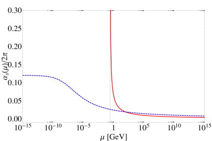
Thus, the actual physical range of a conformal window for pQCD is given by . The behavior of the coupling is shown in Fig. 2.1. In the IR region the strong coupling approaches the IR finite limit, , in the case of values of within the conformal window (e.g. black dashed curve of Fig. 2.1), while it diverges at
| (2.33) |
outside the conformal window given the solution for the coupling with (e.g. the solid red curve of Fig. 2.1). The solution of the NNLO equation for the case , i.e. , can also be given using the standard QCD scale parameter of Eq. (2.33),
| (2.34) | |||||
| (2.35) |
Different solutions can be achieved using different schemes, i.e. different definitions of the scale parameter [128]. We stress that the presence of a Landau “ghost” pole in the strong coupling is only an effect of the breaking of the perturbative regime, including nonperturbative contributions, or using nonperturbative QCD, a finite limit is expected at any [43]. Both solutions have the correct UV asymptotically free behavior. In particular, for the case , we have a negative , a negative and a multi-valued solution, one real and the other imaginary, actually only one (the real) is acceptable given the initial conditions, but this solution is not asymptotically free. We thus restrict our analysis to the range , where we have the correct UV behavior. In general, IR and UV fixed points of the -function can also be determined at different values of the number of colors (different gauge group ) and also extending this analysis to other gauge theories [129].
2.2.3 at higher loops
The 3-loop truncated RG equation 2.15, written using the same normalization as Eq. (2.29) is given by
| (2.36) |
with .
A straightforward integration of this equation would be hard to invert, as shown in Ref. [128], it is more convenient to extend the approach of the previous section by using the Padé Approximant Approach (PAA) [130, 131, 132]. The Padé Approximant of a given quantity calculated perturbatively in QCD up to order , i.e. of the series:
| (2.37) |
is defined as the rational function
| (2.38) |
whose Taylor expansion up to order is identical to the original truncated series. The use of the PA makes the integration of Eq. (2.36) straightforward. PA’s may also be used either to predict the next term of a given perturbative expansion, called a Padé Approximant prediction (PAP), or to estimate the sum of the entire series, called Padé Summation. Features of the PA are described in Ref. [133].
The Padé Approximant () of the 3-loop -function is given by
| (2.39) |
which leads to the solution:
| (2.40) |
and finally,
| (2.41) | |||||
| (2.42) |
the sign of determines the sign of and also the physically relevant branches of the Lambert function : for and the physical branch is , taking real values in the range , while for and the physical branch is given by the , taking real values in the range .
We notice that the only significant difference between the 3-loop solution and the 2-loop solution (2.32) is in the solution . This is because the difference in the definition of can be reabsorbed into an appropriate redefinition of the scale parameter:
For orders up to , an approximate analytical solution is obtained integrating Eq. (2.15):
| (2.43) | |||||
where and , and performing the inversion of the last formula by iteration as shown in Ref. [134], achieving the final result of the coupling at five-loop accuracy:
| (2.44) | |||||
where . The same definition of the scale given in Eq. (2.33) has been used for the scheme, which leads to setting the constant .
Alternatively, we can relate the values of the coupling at two different scales by the 5-loop perturbative solution:
| (2.45) | |||||
2.3 Renormalization scheme dependence
The are the coefficients of the -function arising in the loop expansion, i.e. in powers of . Although the first two coefficients are universally scheme-independent coefficients, depending only on the number of colors and flavors , the higher-order terms are, in contrast, scheme dependent. In particular, for the ’t Hooft scheme [135] the higher terms are set to zero, leading to the solution of Eq. (2.2.2) for the -function valid at all orders. Moreover, in all -like schemes all the coefficients are gauge independent, while other schemes, such as the momentum space subtraction (MOM) scheme [36, 6], depend on the particular gauge. Using the Landau gauge, the terms for the MOM scheme are given by [136]
and
Results for the minimal MOM scheme and Landau gauge are given in Ref. [137]. The renormalization condition for the MOM scheme sets the virtual quark propagator to the same form as a free massless propagator. Different MOM schemes exist and the above values of and are determined with the MOM scheme defined by subtracting the 3-gluon vertex to a point with one null external momentum. This leads to a coupling that is not only RS dependent but also gauge dependent. The values of and given here are only valid in the Landau gauge. Values in the -scheme defined by the static heavy-quark potential [138, 139, 140, 141, 142, 143, 144] can be found in Ref. [145]. They result in and respectively. We recall that the signs of the control the running of . We have for for for and is always positive. Consequently, decreases at high momentum transfer, leading to the asymptotic freedom of pQCD. Note that, are sometimes defined with an additional multiplying factor . Different schemes are characterized by different and lead to different definitions for the effective coupling.
The parameter represents the Landau ghost pole in the perturbative coupling in QCD. We recall that the Landau pole was initially identified in the context of Abelian QED. However, the presence of this pole does not affect QED. Given its value, , above the Planck scale [146], at which new physics is expected to occur in order to suppress the unphysical divergence. The QCD parameter in contrast is at low energies, its value depends on the RS, on the order of the -series, , on the approximation of the coupling at orders higher than and on the number of flavors . Although mass corrections due to light quarks at higher order in perturbative calculations introduce negligible terms, they actually indirectly affect through . In fact, the number of active quark flavors runs with the scale and a quark is considered active in loop integration if the scale . Thus, in general, light quarks can be considered massless regardless of whether they are active or not, while varies smoothly when passing a quark threshold, rather than in discrete steps. The matching of the values of below and above a quark threshold makes depend on . Matching requirements at leading order , imply that:
and therefore that:
The formula with , can be found in [147] and the four-loop matching in the RS is given in [148].
As shown in the previous section at the lowest order , the Landau singularity is a simple pole on the positive real axis of the -plane, whereas at higher order it acquires a more complicated structure. This pole is unphysical and is located on the positive real axis of the complex -plane. This singularity of the coupling indicates that the perturbative regime of QCD breaks down and it may also suggest that a new mechanism takes over, such as the confinement. Thus, the value of is often associated with the confinement scale, or equivalently to the hadronic mass scale. An explicit relation between hadron masses and the scale has been obtained in the framework of holographic QCD [149]. Landau poles on the other hand, usually do not appear in nonperturbative approaches, such as AdS/QCD.
Different schemes are related perturbatively by:
| (2.46) |
where is the leading order difference between in the two schemes. In the case of the V-scheme and scheme we have: . Thus, the relation between in a scheme 1 and in a scheme 2 is, at the one-loop order, given by:
For example, the and V-scheme scale parameters are related by:
The relation is valid at each threshold, translating all values for the scale from one scheme to the other.
2.4 The Extended Renormalization Group Equations
Given that physical predictions cannot depend on the choice of the renormalization scale nor on the scheme, the same approach used for the renormalization scale based on the invariance under RGE is extended to scheme transformations. This approach leads to the Extended Renormalization Group Equations, which were introduced first by Stückelberg and Peterman [1], then discussed by Stevenson [8, 9, 11, 10] and also improved by Lu and Brodsky [150]. A physical quantity, , calculated at the -th order of accuracy is expressed as a truncated expansion in terms of a coupling constant defined in the scheme and at the scale , such as
| (2.47) |
At any finite order, the scale and scheme dependences of the coupling constant and of the coefficient functions do not totally cancel, this leads to a residual dependence in the finite series and to the scale and scheme ambiguities.
In order to generalize the RGE approach, it is convenient to improve the notation by introducing the universal coupling function as the extension of an ordinary coupling constant to include the dependence on the scheme parameters :
| (2.48) |
where is the standard two-loop scale parameter. The subtraction prescription is now characterized by an infinite set of continuous scheme parameters and by the renormalization scale . Stevenson [9] has shown that one can identify the beta-function coefficients of a given renormalization scheme with the scheme parameters. Considering that the first two coefficients of the -function are scheme independent, each scheme is identified by its parameters.
More conveniently, let us define the rescaled coupling constant and the rescaled scale parameter as
| (2.49) |
Then, the rescaled -function takes the canonical form:
| (2.50) |
with for .
The scheme and scale invariance of a given observable , can be expressed as:
| (2.51) |
The fundamental beta function that appears in Eqs. (2.51) reads:
| (2.52) |
and the extended or scheme-parameter beta functions are defined as:
| (2.53) |
The extended beta functions can be expressed in terms of the fundamental beta function. Since the are independent variables, second partial derivatives respect the commutativity relation:
| (2.54) |
which implies
| (2.55) |
| (2.56) |
where and . From here
| (2.57) |
| (2.58) |
where the lower limit of the integral has been set to satisfy the boundary condition
That is, a change in the scheme parameter can only affect terms of order or higher in the evolution of the universal coupling function.
The extended renormalization group equations Eqs. (2.51) can be written in the form:
| (2.59) |
Thus, provided we know the extended beta functions, we can determine any variation of the expansion coefficients of under scale-scheme transformations. In particular, we can evolve a given perturbative series into another, determining the expansion coefficients of the latter and vice versa. Thus, different schemes and scales can be related according to the extended renormalization group equations and the fundamental requirement of “renormalization scale and scheme invariance” is recovered via the extended renormalization group invariance of perturbative QCD. Unfortunately, these relations and in general all perturbative calculations are known only up to a certain level of accuracy and the truncated formulas are responsible for an important source of uncertainties: the scheme and scale ambiguities.
2.5 The running coupling constant
The strong coupling , is a fundamental parameter of the SM theory and determines the strength of the interactions among quarks and gluons in quantum chromodynamics (QCD).
In order to understand hadronic interactions, it is necessary to determine the magnitude of the coupling and its behavior over a wide range of values, from low- to high-energy scales. Long and short distances are related to low and high energies respectively. In the high-energy region the strong coupling has an asymptotic behavior and QCD becomes perturbative, while in the region of low energies, e.g. at the proton-mass scale, the dynamics of QCD is affected by processes such as quark confinement, soft radiation and hadronization. In the first case experimental results can be matched with theoretical calculations and a precise determination of depends on both experimental accuracy and theoretical errors. In the latter case experimental results are difficult to achieve and theoretical predictions are affected by the confinement and hadronization mechanisms, which are rather model dependent. Various processes also involve a precise knowledge of the coupling in both the high and low momentum transfer regions and in some cases calculations must be improved with electroweak (EW) corrections. Thus, the determination of the QCD coupling over a wide range of energy scales is a crucial task in order to achieve results and to test QCD to the highest precision. Theoretical uncertainties in the value of contribute to the total theoretical uncertainty in the physics investigated at the Large Hadron Collider (LHC), such as the Higgs sector, e.g. Higgs production via gluon fusion [19]. The behavior of the perturbative coupling at low-momentum transfer is also fundamental for the scale of the proton mass, in order to understand hadronic structure, quark confinement and hadronization processes. IR effects, such as soft radiation and renormalon factorial growth, spoil the perturbative nature of QCD in the low-energy domain. Higher-twist effects can also play an important role. Processes involving the production of heavy quarks near threshold require knowledge of the QCD coupling at very low momentum scales. Even reactions at high energies may involve the integration of the behavior of the strong coupling over a large domain of momentum scales, including IR regions. Precision tests of the coupling are crucial also for other aspects of QCD that are still under continuous investigation, such as the hadron masses and their internal structure. In fact, the strong interaction is responsible for the mass of hadrons in the zero-mass limit of the , quarks.
The origin and phenomenology of the behavior of at small distances, where asymptotic freedom appears, is well understood and explained in many textbooks on Quantum Field Theory and Particle Physics. Numerous reviews exist; see e.g. Refs. [151, 152]. However, standard explanations often create an apparent puzzle. Other questions remain even in this well understood regime: a significant issue is how to identify the scale that controls a given hadronic process, especially if it depends on many physical scales.
3 The Principle of Maximum Conformality – PMC scale setting
The Principle of Maximum Conformality (PMC) [45, 46, 47, 49, 50] is the principle underlying BLM and it generalizes the BLM method to all possible applications and to all orders.
BLM scale setting is greatly inspired by QED. The standard Gell-Mann–Low scheme determines the correct renormalization scale identifying the scale with the virtuality of the exchanged photon [2]. For example, in electron–muon elastic scattering, the renormalization scale is given by the virtuality of the photon exchanged, i.e. the spacelike momentum transfer squared . Thus,
| (3.1) |
where
is the vacuum polarization (VP) function. From Eq. (3.1) it follows that the renormalization scale can be determined by the -term at the lowest order. This scale is sufficient to sum all the vacuum polarization contributions into the dressed photon propagator, both proper and improper to all orders. Starting from a first evaluation of the physical observable that is obtained by calculating perturbative corrections in a given scheme (commonly used are or ) and at an initial renormalization scale , one obtains the truncated expansion:
| (3.2) |
where is the tree-level term, while are the one-loop, two-loop and -loop corrections respectively and is the power of the coupling at tree-level. In order to improve the pQCD estimate of the observable, after the initial renormalization a change of scale using the RGE is performed according to the BLM scale setting.
Following the GM–L scheme in QED, the BLM scales can be determined at LO in perturbation theory by writing explicit contributions coming from the different terms of the NLO coefficient in a physical observable as [15]:
| (3.3) | |||||
where stands for an initial renormalization scale, which practically can be taken as the typical momentum transfer of the process. The term is due to the quark vacuum polarization. Calculations are in the -scheme.
At the NLO level, all terms should be resummed into the coupling. Using the NLO -running formula:
| (3.4) |
we obtain
| (3.5) |
where
is the BLM scale and
is the conformal coefficient, i.e. the NLO coefficient not depending on the RS and scale . Both the effective BLM scale and the coefficient are independent and conformal at LO. By including the term into the scale we eliminate the term of the NLO coefficient , which is responsible for the running of the coupling constant, and the observable in the final results can be written in its maximal conformal form, Eq. (3.5).
The BLM method can be extended to higher orders in a systematic way by including the terms arising at higher order into the BLM scales consistently. In order to extend the BLM beyond the NLO, the following points are considered essential:
-
1.
All -terms associated with the -function (i.e. terms) and then with the renormalization of the coupling constant, must be absorbed into the effective coupling, while those -terms that have no relation with UV-divergent diagrams (i.e. -terms) should be identified and considered as part of the conformal coefficients. After BLM scale setting, the perturbative series for the physical observable becomes a conformal series, all nonconformal terms should be absorbed into the effective coupling in a consistent manner.
-
2.
New -terms (corresponding to new coefficients) arise at each perturbative order, thus a new BLM scale that sums these terms consistently into the running coupling, should be introduced at each calculated perturbative order. In fact, there is no reason to use a unified effective scale for the entire perturbative series as shown in Refs. [153, 154].
-
3.
The BLM scales themselves should be a RG-improved perturbative series [46]. The length of the perturbative series for each BLM scale depends on how many new -terms (or -terms) we have from the higher-order calculation and to what perturbative order we have performed.
Actually, the last point is not mandatory and needs clarification. In order to apply the BLM/PMC using perturbative scales, the argument of the coupling in the expansion of the BLM/PMC scale should be the physical scale of the process , that may be either the center-of-mass energy or even another variable, such as , depending on the process. Setting the initial scale to the physical scale would greatly simplify the BLM/PMC procedure, preserving the original scale invariance of the observable and eliminating the initial scale dependence from the BLM/PMC scales. In case the BLM/PMC scales are not perturbatively calculated, as will be shown in Section 4.1, the initial scale can be treated as an arbitrary parameter.
In agreement with these indications, it is possible to achieve a scale setting method extendible iteratively to all orders, which leads to the correct coefficients for the final “maximally conformal” series:
| (3.6) |
where the BLM scales are set by a recursive use of the RG equations in order to cancel all the terms from the series. We remark that since the coefficients have been obtained cancelling all terms related to running of the coupling they actually are free of any scale and scheme dependence left. In other words, the , where the are conformal coefficients not depending on the renormalization scale. Hence, the BLM approach leads to an maximally conformal observable, i.e. where all the renormalization scale and scheme dependence has been confined to the effective coupling and to its renormalization scale .
Fundamental features of the BLM method:
-
A)
BLM scales at LO, are set simply by identifying the coefficient of the term.
-
B)
Since all -terms related to the running of the coupling are reabsorbed, scheme differences do not affect the results and the perturbative expansions in in two different schemes, e.g. and , are identical. We notice that -terms related to the UV finite diagrams, may arise at every order in perturbation theory. These terms might be related either to the particular kinematics of the initial state or even to finite loop diagrams arising at higher orders, thus in both cases are insensitive to the UV cutoff or to the RS and cannot be considered as -terms. We label these terms as -terms and they do not give contributions to the BLM scales.
-
C)
Using BLM scale setting, the perturbative expansion does not change across quark threshold, given that all vacuum-polarization effects due to a new quark are automatically absorbed into the effective coupling. This implies that in a process with fixed kinematic variables (e.g. a total cross-section), we can use a naive LO/NLO -running, with the number of active flavor fixed to the value determined by the BLM scale, to perform the calculation [155].
-
D)
The BLM method preserves all the RG properties of existence and uniqueness, reflexivity, symmetry and transitivity. As shown in Refs. [156, 157, 158, 159], the RG invariance of the BLM leads to scheme-independent transformations that relate couplings in different schemes. These are known as commensurate scale relations (CSRs) and it has been shown that, even though the expansion coefficients under different renormalization schemes can be different, after a proper scale setting, one can determine a relation between the effective couplings leading to an invariant result for the calculated quantity. Using this approach it is also possible to extend conformal properties to renormalizable gauge theories, such as the generalized Crewther relation [160, 161, 162, 163].
-
E)
The BLM approach reduces to the GM–L scheme for QED in the Abelian limit [32]; the results are in perfect agreement.
-
F)
The elimination of the term related to the coefficient from the perturbative series eliminates the renormalon terms over the entire range of the accessible physical energies and not only in the low-energy domain. The convergence of the resulting series is then greatly improved.
Several extended versions of the BLM approach beyond the NLO have been proposed in the literature, such as the dressed-skeleton expansion, the large- expansion, the BLM expansion with an overall renormalization scale and the sequential BLM (seBLM), an extension to the sequential BLM (xBLM) in Refs. [164, 165, 159, 163, 153, 166, 167, 168]. These different extensions of the BLM are mostly partial or ad hoc improvements of the first LO-BLM [15] in some cases up to NNLO, in other cases using a rather effective approach, i.e. by introducing an overall effective BLM scale for the entire perturbative expansion. Results obtained with these approaches also did not respect the basic points (1–3). Most importantly, these methods lead to results that are still dependent on the initial renormalization scale. The fundamental feature of the BLM is to obtain results free of scale ambiguities and thus independent of the choice of initial renormalization scale. The first aim of the BLM scale is to eliminate the renormalization scale and scheme uncertainties; thus any extension of the BLM not respecting this basic requirement does not represent a real improvement of the standard conventional scale setting CSS method.
The reasons for the different extensions of the BLM method to higher orders were mainly two: firstly, it was not clear how to generalize this approach to all possible quantities, which translates into the question: what is the principle underlying the BLM method? And secondly, what is the correct procedure to identify and reabsorb the -terms unambiguously order-by-order? A practical reason that renders the extension to higher orders not straightforward is the presence of finite UV corrections given by the three- and four-gluon vertices of the additional -terms that are unrelated to the running of .
In its first formulation in Ref. [45] it was suggested to use a unique PMC scale at LO to reabsorb all contributions related to different skeleton-graph scales by properly weighting the two contributions, such as that of the -channel and -channel. This approach was more oriented towards a single PMC scale that reabsorbs all terms related to the running coupling. A multi-scale approach was later developed considering different scales arising at each order of accuracy including different coefficients according to the perturbative expansion. We remark that the PMC method preserves all the properties (A–F) of the BLM procedure and it extends these properties to all orders, eliminating the renormalization scale and scheme ambiguities. The PMC also generalizes this approach to all gauge theories. Firstly, this is crucial in order to apply the same method to all SM sectors. Secondly, in the perspective of a grand unified theory (GUT), only one scale-setting method may be applied for consistency, and this method must agree with the GM–L scheme and with the QED results.
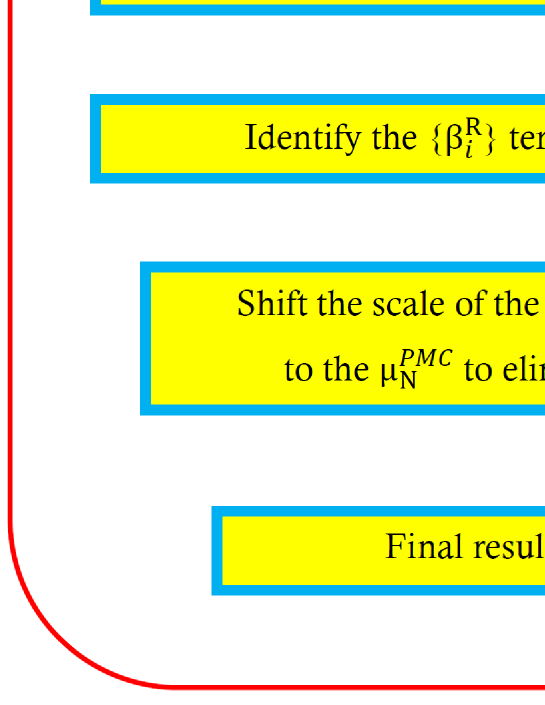
In order to apply the PMC, is convenient to follow the flowchart shown in Fig. 3.1 and to write the observable of Eq. (3.2) with the explicit contributions of the terms in the coefficients calculated at each order of accuracy:
| (3.7) |
where represents the kinematic scale or the physical scale of the measured observable and is the power of associated with the tree-level terms. In general, this procedure is always possible either for analytic or numerical (e.g. Monte Carlo) calculations, given that both strategies keep track of terms related to different color factors. The core of the PMC method, as was for BLM, is that all terms related to the -function arising in a perturbative calculation must be summed, by proper definition of the renormalization scale , into the effective coupling by recursive use of the RGE. Essentially the difference between the two procedures is that while in BLM the scales are set iteratively order-by-order to remove all terms, in the PMC the terms are written first as terms and then reabsorbed into the effective coupling. The two procedures are related by the correspondence principle [46].
3.1 The multi-scale Principle of Maximum Conformality: PMCm
The PMCm method is based on a multi-scale application of the PMC. In this section we show how to implement this method to any order of accuracy. First, as shown in the flowchart in Fig. 3.1, for the pQCD approximant (3.7), it is convenient to transform the series at each order into the series. The QCD degeneracy relations [169] ensure the realizability of such a transformation. For example, Eq. (3.7) may be rewritten as [49, 50]
| (3.8) | |||||
where can be derived from , are conformal coefficients and are nonconformal. For definiteness and without loss of generality, we have set and to illustrate the PMC procedures. Different types of -terms can be absorbed into in an order-by-order manner by using the RGE, which leads to distinct PMC scales at each order:
| (3.9) | |||||
The coefficients are generally functions of , which can be redefined as
| (3.10) |
where the reduced coefficients (specifically, we have ) and the combinatorial coefficients . As discussed in the previous section, we set the renormalization scale to the physical scale of the process :
| (3.11) | |||||
| (3.12) | |||||
| (3.13) |
Note that the PMC scales are of a perturbative nature, which is also a sort of resummation and we need to know more loop terms to achieve more accurate predictions. The PMC resums all the known same type of -terms to form precise PMC scales for each order. Thus, the precision of the PMC scale for the high-order terms decreases at higher and higher orders due to the less known -terms in those higher-order terms. For example, is determined up to next-to-next-to-leading-logarithm (N2LL) accuracy, is determined up to NLL accuracy and is determined at LL accuracy. Thus, the PMC scales at higher orders are of less accuracy due to more of the perturbative terms being unknown. This perturbative property of the PMC scale causes the first kind of residual scale dependence.
After fixing the magnitude of , we achieve a conformal series
| (3.14) |
The PMC scale for the highest-order term, e.g. for the present case, is unfixed, since there is no -term to determine its magnitude. This renders the last perturbative term unfixed and causes the second kind of residual scale dependence. Usually, the PMCm suggests setting as the last determined scale , which ensures the scheme independence of the prediction due to commensurate scale relations among the predictions under different renormalization schemes [159, 170]. The pQCD series (3.14) is renormalization scheme and scale independent and becomes more convergent due to the elimination of the terms including those related to the renormalon divergence. Thus, a more accurate pQCD prediction can be achieved by applying the PMCm. Two residual scale dependences are due to perturbative nature of either the pQCD approximant or the PMC scale, which is in principal different from the conventional arbitrary scale dependence. In practice, we have found that these two residual scale dependences are quite small even at low orders. This is due to a generally faster pQCD convergence after applying the PMCm. Some examples can be found in Ref. [171].
3.2 The single-scale Principle of Maximum Conformality: PMCs
In some cases, the perturbative series might have a weak convergence and the PMC scales might retain a comparatively larger residual scale dependence. To overcome this, a single-scale approach has been proposed, namely the PMCs, in order to suppress the residual scale dependence by directly fixing a single effective . Following the standard procedures of PMCs [172], the pQCD approximant (3.8) changes to the following conformal series,
| (3.15) |
As in the previous section, we have set and for illustrating the procedure. The PMC scale can be determined by requiring all the nonconformal terms to vanish, which can be fixed up to N2LL accuracy for and , i.e. can be expanded as a power series over ,
| (3.16) |
where the coefficients are
| (3.17) | ||||
| and | ||||
| (3.18) | ||||
Eq. (3.16) shows that the PMC scale is also a power series over , which resums all the known -terms and is explicitly independent of at any fixed order, but depends only on the physical scale Q. It represents the correct momentum flow of the process and determines an overall effective value. Together with the -independent conformal coefficients, the resultant PMC pQCD series is scheme and scale independent [58]. By using a single PMC scale determined with the highest accuracy from the known pQCD series, both the first and the second kind of residual scale dependence are suppressed.
4 Infinite-Order Scale Setting via the Principle of Maximum Conformality: PMC∞
In this section we introduce a parametrization of the observables that stems directly from the analysis of the perturbative QCD corrections and which reveals interesting properties, such as scale invariance, independently of the process or of the kinematics. We point out that this parametrization can be an intrinsic general property of gauge theories and we define this property intrinsic conformality (iCF333Here the conformality must be understood as RG invariance only.). We also show how this property directly indicates the correct renormalization scale at each order of calculation and we define this new method PMC∞: Infinite-Order Scale Setting using the Principle of Maximum Conformality. We apply the iCF property and the PMC∞ to the case of the thrust and -parameter distributions in jets and we display the results.
4.1 Intrinsic conformality (iCF)
In order to introduce intrinsic conformality (iCF), we consider the case of a normalized IR-safe single-variable distribution and write the explicit sum of pQCD contributions calculated up to NNLO at the initial renormalization scale :
| (4.1) |
where the is a tree-level hadronic cross-section, are respectively the LO, NLO and NNLO coefficients, is the selected unintegrated variable. For the sake of simplicity, we shall refer to the perturbatively calculated differential coefficients as implicit coefficients and drop the derivative symbol, i.e.
| (4.2) |
We define here the intrinsic conformality as the property of a renormalizable SU(N)/U(1) gauge theory, such as QCD, which yields a particular structure of the perturbative corrections that can be made explicit by representing the perturbative coefficients using the following parametrization: 444We are neglecting here other running parameters, such as the mass terms.
| (4.3) |
where the are the scale-invariant Conformal Coefficients (i.e. the coefficients of each perturbative order not depending on the scale ), while we define the as Intrinsic Conformal Scales and are the first two coefficients of the -function. We recall that the implicit coefficients are defined at the scale and that they change according to the standard RG equations under a change of the renormalization scale according to:
| (4.4) |
It can be shown that the form of Eq. (4.3) is scale invariant and it is preserved under a change of the renormalization scale from to by standard RG equations Eq. (4.4), i.e.:
| (4.5) |
We note that the form of Eq. (4.3) is invariant and that the initial scale dependence is exactly removed by . Extending this parametrization to all orders we achieve a scale-invariant quantity: the iCF parametrization is a sufficient condition in order to obtain a scale-invariant observable.
In order to show this property we collect together the terms identified by the same conformal coefficient, we call each set a conformal subset and extend the property to order :
| (4.6) | |||||
In each subset we have only one intrinsic scale and only one conformal coefficient and the subsets are disjoint; thus, no mixing terms among the scales or the coefficients are introduced in this parametrization. Moreover, the structure of the subsets remains invariant under a global change of the renormalization scale, as shown from Eq. (4.5). The structure of each conformal set and consequently the iCF are preserved, also if we fix a different renormalization scale for each conformal subset, i.e.
| (4.7) |
We define here this property of Eq. 4.6 of separating an observable into the union of ordered scale-invariant disjoint subsets an ordered scale invariance.
In order to extend the iCF to all orders, we perform the limit using the following strategy: we first perform a partial limit including the higher-order corrections relative only to those terms that have been determined already at order for each subset and we then perform the complementary limit, which consists in including all the remaining higher-order terms. For the limit we have:
| (4.8) |
where is the coupling calculated up to at the intrinsic scale . Given the particular ordering of the powers of the coupling, in each conformal subset we have the coefficients of the terms, where is the order of the conformal subset and the is the order of the highest subset with no terms. We note that the limit of each conformal subset is finite and scale invariant up to . The remaining scale dependence is confined to the coupling of the term. Any combination of the subsets is finite and scale invariant. We can now extend the iCF to all orders performing the limit. In this limit we include all the remaining higher-order corrections. For the calculated conformal subsets this leads to defining the coupling at the same scales but including all the missing terms. Thus, each conformal subset remains scale invariant. We point out that we are not making any assumption on the convergence of the series for this limit. We thus have:
| (4.9) |
where here now is the complete coupling determined at the same scale . Equation (4.9) shows that the entire renormalization scale dependence has been completely removed. In fact, neither the intrinsic scales nor the conformal coefficients depend on the particular choice of the initial scale. The only term with a residual dependence is the -th term, but this dependence cancels in the limit . The scale dependence is totally confined to the coupling and its behavior does not depend on the particular choice of any scale in the perturbative region, i.e. with . Hence, the limit of depends only on the properties of the theory and not on the scale of the coupling in the perturbative regime. The proof given here shows that the iCF is sufficient to have a scale-invariant observable and it does not depend on the particular convergence of the series.
In order to show the necessary condition, we separate the two cases of a convergent series and an asymptotic expansion. For the first case the necessary condition stems directly from the uniqueness of the iCF form, since given a finite limit and the scale invariance, any other parametrization can be reduced to the iCF by means of appropriate transformations in agreement with the RG equations. For the second case, we have that an asymptotic expansion though not convergent, can be truncated at a certain order , which is the case of Eq. (4.6). Given the particular structure of the iCF we can perform the first partial limit and we would achieve a finite and scale-invariant prediction, , for a truncated asymptotic expansion, as shown in Eq. (4.8). Given the truncation of the series in the region of maximum of convergence the -th term would be reduced to the lowest value and so the scale dependence of the observable would reach its minimum. Given the finite and scale-invariant limit we conclude that the iCF is unique and thus necessary for an ordered scale-invariant truncated asymptotic expansion up to the -th order.
We point out that in general the iCF form is the most general and irreducible parametrization that leads to scale invariance; other parametrization are forbidden, since if we were to introduce more scales 555Here we refer to the form of Eq. (4.3). In principle, it is possible to write other parametrizations preserving the scale invariance, but these can be reduced to the iCF in agreement with the RG equations. into the logarithms of one subset, we would spoil the invariance under the RG transformation and we could not achieve Eq. (4.5), while on the other hand no scale dependence can be introduced into the intrinsic scales since it would remain in the observable already in the first partial limit and it could not be eliminated. The conformal coefficients are conformal at each order by definition; thus, they do not depend on the renormalization scale and they do not have a perturbative expansion. Hence the iCF is a necessary and sufficient condition for scale invariance.
4.2 Comments on the iCF and ordered scale invariance
The iCF parametrization can stem either from an inner property of the theory, the iCF, or from direct parametrization of the scale-invariant observable. In both cases the iCF parametrization makes the scale dependence of the observable explicit and it exactly preserves the scale invariance. The iCF parametrization is invariant with respect to the choice of initial scale , this implies that the same calculation performed choosing different arbitrary initial scales, leads to the same result in the limit , a limit that is scale and scheme independent. The iCF is also strongly motivated by the renormalizability of QCD and by the uniqueness of the -function in a given scheme; i.e. two different do not occur in a perturbative calculation at any order in one RS and the UV divergencies are cancelled by redefinition of the same parameters at lowest and higher orders. We remark that the conservation of the iCF form in one observable is strongly related to the validity of the RG transformations; we thus expect the iCF to be well preserved in the deep Euclidean region.
Once we have defined an observable in the iCF-form, we have not only the scale invariance of the entire observable, but also the ordered scale invariance (i.e. the scale invariance of each subset or ). The latter property is crucial in order to obtain scale-invariant observables independently from the particular kinematic region and independently from the starting order of the observable or the order of the truncation of the series. Since in general, a theory is blind with respect to the particular observable/process that we might investigate, the theory should preserve the ordered scale invariance in order to always define scale-invariant observables. Hence if the iCF is an inner property of the theory, it leads to implicit coefficients that are neither independent nor conformal. This is made explicit in Eq. (4.3), but it is hidden in the perturbative calculations in the case of the implicit coefficients. For instance, the presence of the iCF clearly reveals itself when a particular kinematic region is approached and the becomes null. This would cause a breaking of the scale invariance since a residual initial scale dependence would remain in the observable in the higher-order coefficients. The presence of the iCF solves this issue by leading to the correct redefinition of all the coefficients at each order preserving the correct scale invariance exactly. Thus, in the case of a scale-invariant observable , defined according to the implicit form (Eq. (4.1)), by the coefficients it cannot simply undergo the change , since this would break the scale invariance. In order to preserve the scale invariance, we must redefine the coefficients cancelling out all the initial scale dependence originating from the LO coefficient at all orders. This is equivalent to subtracting out an entire invariant conformal subset related to the coefficient from the scale-invariant observable . This mechanism is clear in the case of the explicit form of the iCF, Eq. (4.3), where, if , then the entire conformal subset is null and the scale invariance is preserved.
We stress that the conformal coefficients may acquire all possible values without breaking scale invariance, they contain the essential information on the physics of the process, while all the correlation factors can be reabsorbed into the renormalization scales as shown by the PMC method [46, 47, 49, 50]. Hence, if a theory has the property of ordered scale invariance, it exactly preserves the scale invariance of observables independently of the process, the kinematics and the starting order of the observable. We stress that if a theory has intrinsic conformality, all renormalized quantities, such as cross sections, can be parametrized with the iCF-form. This property should be preserved by the renormalization scheme or by the definition of IR safe quantities and it should also be preserved in observables defined in effective theories. The iCF shows that point (3) of the BLM/PMC approach (Section 3) can be improved by eliminating the perturbative expansion of the BLM/PMC scales, leading to a scale- and scheme-invariant result. We remark though that the perturbative corrections in the BLM or PMCm scales are suppressed in the perturbative region.
4.3 The PMC∞
We introduce here a new method for eliminating the scale-setting ambiguity in single variable scale-invariant distributions, which we call PMC∞. This method is based on the original PMC principle and agrees with all the different PMC formulations for the PMC scales at lowest order. The core of the PMC∞ is essentially the same for all BLM-PMC prescriptions, i.e. the effective running-coupling value and hence its renormalization scale at each order is determined by the -term of the next-higher order, or equivalently by the intrinsic conformal scale . The PMC∞ preserves the iCF and thus the scale and scheme invariance, absorbing an infinite set of -terms to all orders.
This method differs from the other PMC prescriptions since, due to the presence of the intrinsic conformality, no perturbative correction in needs to be introduced at higher orders in the PMC scales. Given that all the -terms of a single conformal subset are included in the renormalization scale already with the definition at lowest order, no initial scale or scheme dependences are left due to the unknown -terms in each subset. The PMC∞ scale of each subset can be unambiguously determined by -term of each order, we stress that all logarithms of each subset have the same argument and all the differences arising at higher orders have to be included only in the conformal coefficients. Reabsorbing all the -terms into the scale also eliminates the terms (related to renormalons [23]); thus, the precision is improved and the perturbative QCD predictions can be extended to a wider range of values. The initial scale dependence is totally confined in the unknown PMC∞ scale of the last order of accuracy (i.e. up to NNLO case in the ). Thus, if we fix the renormalization scale independently to the proper intrinsic scale for each subset , we end up with a perturbative sum of totally conformal contributions up to the order of accuracy:
| (4.10) | |||||
At this order, the last scale is set to the physical scale , i.e. .
4.4 The iCF coefficients and scales: a new “How-To” method
We describe here how all the coefficients of Eq. (4.3) can be identified from either a numerical or analytical perturbative calculation. This method applies in general to any perturbative calculation once results for the different color factors are kept separate; however, we refer to the particular case of the NNLO thrust distribution results calculated in Refs. [173, 174] for the purpose. Since the leading order is already () void of -terms, we start with NLO coefficients. A general numerical/analytical calculation keeps tracks of all the color factors and the respective coefficients:
| (4.11) |
where , and The dependence on is made explicit here for sake of clarity. We can determine the conformal coefficient of the NLO order straightforwardly, by fixing the number of flavors in order to kill the term:
| (4.12) |
We would achieve the same results in the usual PMC way; i.e. by identifying the coefficient with the term and then determining the conformal coefficient. Both methods are consistent and results for the intrinsic scales and the coefficients are in perfect agreement. At NNLO a general coefficient is composed of the contribution of six different color factors:
| (4.13) | |||||
In order to identify all the terms of Eq. (4.3), we notice first that the coefficients of the terms and are already given by the NLO coefficient ; we thus need to determine only the and the conformal terms. In order to determine the latter coefficients, we use the same procedure used for the NLO; i.e. we set the number of flavors in order to remove all the terms. We then have
| (4.14) |
with . Up to accuracy , we have:
| (4.15) | |||||
with
This procedure may be extended to all orders and one may decide whether to cancel , or by fixing the appropriate number of flavors. The results can be compared to exactly determine all the coefficients. We point out that extending the intrinsic conformality to all orders, we can at this stage predict the coefficients of all the color factors of the higher orders related to the -terms, except those related to the higher-order conformal coefficients and -terms (e.g. at LO, and ).
4.5 Comment on the PMC/PMC∞ scales
PMC scales stem directly from the renormalization of the UV-divergent diagrams. As pointed out in Sec. 2.1, the finite part of the divergent integrals contribute to the -terms. In fact, these coefficients derive from the UV-divergent diagrams connected with the running of the coupling constant and not from UV-finite diagrams. UV-finite terms may arise but would not contribute to the -terms. These terms can be easily identified by the kinematic constraint at lowest order or by checking deviations of the coefficients from the iCF form. In fact, only the terms coming from UV-divergent diagrams, depending dynamically on the virtuality of the underlying quark and gluon subprocesses have to be considered as -terms and they would determine the intrinsic conformal scales. In general, each is an independent function of the physical scale of the process (or ), of the selected variable and it varies with the number of colors mainly due to the and vertices. The latter terms arise at higher orders only in a non-Abelian theory, but they are not expected to spoil the iCF-form. We stress that iCF applies to scale-invariant single-variable differential distributions, in case one is interested in the renormalization of a particular diagram, e.g. the vertex, contributions from different -terms should be singled out in order to identify the respective intrinsic conformal scale consistently with the renormalization of the non-Abelian vertex, as shown in [175].
In the renormalization procedure of gauge theories, one first identifies the UV singularities of a scattering amplitude, which appear as poles using dimensional regularization. The UV-divergent contributions are absorbed into renormalization constants adopting a particular scheme (e.g. the scheme). This cancels the UV divergences and at the same time defines the finite part of the loop integral.
The finite parts, such as the finite and contributions, are associated with the renormalization of the running coupling and running mass, respectively. The terms can then be summed into the running coupling using the standard renormalization group equations; this is basically the core of the BLM-PMC scale-setting procedure that is analogous to the Gell-Mann–Low scheme in QED. This procedure eliminates the scale ambiguity and reabsorbs the scheme dependence at once into the effective running coupling up to the computed order. In addition, the factorial renormalon divergence is eliminated. One thus can use the same renormalization procedure for QED, QCD and EW in a grand unified theory,
Given the renormalizability of QCD, once the coupling is renormalized all the vertices are finite, but this does not cancel the contributions of the finite parts of the integrals, i.e. the terms, which define the PMC scale for each vertex (, , , ).
5 PMC∞ results for thrust and the -parameter
The thrust distribution and event-shape variables are fundamental tools for probing the geometrical structure of a given process at colliders. Being observables that are exclusive enough with respect to the final state, they allow for a deeper geometrical analysis of the process and are also particularly suited for measurement of the strong coupling [176].
Given the high-precision data collected at LEP and SLAC [177, 178, 179, 180, 181], refined calculations are crucial in order to extract information to the highest possible precision. Although extensive studies on these observables have been produced during the last few decades, including higher-order corrections from next-to-leading order (NLO) calculations [182, 183, 184, 185, 186, 187] to the next-to-next-to-leading order(NNLO) [188, 189, 190, 173, 174] and including resummation of the large logarithms [31, 30], the theoretical predictions are still affected by significant theoretical uncertainties that are related to large renormalization scale ambiguities. In the particular case of the three-jet event-shape distributions the conventional practice of CSS leads to results that do not match the experimental data and the extracted values of deviate from the world average [126].
The thrust () and -parameter () are defined by
| (5.1) |
| (5.2) |
where the sum runs over all particles in the hadronic final state and denotes the three-momentum of particle . The unit vector is varied to maximize thrust ; the corresponding is called the thrust axis and denoted by . The variable is often used, which for the LO of 3-jet production is restricted to the range . We have a back-to-back or a spherically symmetric event at and at respectively. For the -parameter, is the angle between and . At LO for 3-jet production the -parameter is restricted by kinematics to the range .
In general, a normalized IR-safe single-variable observable, such as the thrust distribution for jets [191, 192], is the sum of pQCD contributions calculated up to NNLO at the initial renormalization scale :
| (5.3) |
where , is the selected event-shape variable, the cross-section of the process,
is the total hadronic cross-section and are respectively the normalized LO, NLO and NNLO coefficients:
| (5.4) | |||||
where are the coefficients normalized to the tree-level cross-section calculated by Monte Carlo (see e.g. the EERAD and Event2 codes [188, 189, 190, 173, 174]) and are
| (5.5) |
where is the Riemann zeta function.
In general, according to CSS the renormalization scale is set to and theoretical uncertainties are evaluated using standard criteria. In this case, we have used the definition of the parameter given in Ref. [189]; we define the average error for the event-shape variable distributions as:
| (5.6) |
where is the index of the bin and is the total number of bins, the renormalization scale is varied in the range .
5.1 The PMC∞ scales at LO and NLO
According to the PMC∞ prescription, we fix the renormalization scale to at each order absorbing all the terms into the coupling. We notice a small mismatch between the zeroes of the conformal coefficient and those of the remaining term in the numerator (the formula is shown in Eq. (4.14)). Due to our limited knowledge of the strong coupling at low energies, in order to avoid singularities in the NLO scale , we introduce a regularization that leads to a finite scale over the entire range of values of the variable . These singularities might be due either to the presence of UV finite terms or to the logarithmic behavior of the conformal coefficients when low values of the variable are approached. Large logarithms arise from the IR-divergence cancellation procedure and they can be resummed in order to restore a predictive perturbative regime [25, 26, 27, 30, 31]. We point out that IR cancellation should not spoil the iCF property. Whether this is an actual deviation from the iCF-form must be investigated further. However, since the discrepancies between the coefficients are rather small, we introduce a regularization method based on redefinition of the norm of the coefficient in order to cancel out these singularities in the scale. This regularization is consistent with the PMC principle and up to the accuracy of the calculation it does not introduce any bias effect in the results or any ambiguity in the NLO-PMC∞ scale. All differences introduced by the regularization would enter at accuracy and they may be reabsorbed later in the higher-order PMC∞ scales. For the PMC∞ scales, we thus obtain
| (5.7) | |||||
| (5.10) |
where and the third scale is set to . The renormalization scheme factor for the QCD results is set to . This scheme factor also reabsorbs the scheme difference into the renormalization scale and is related to the particular choice of the scale parameter as discussed in Section 2.3. The coefficients are the coefficients related to the -terms of the NL and NNL perturbative order of the thrust distribution respectively. They are determined from the calculated coefficients.
The parameter is a regularization term to cancel the singularities of the NLO scale, , in the range , depending on non-matching zeroes between numerator and denominator in . In general, this term is not mandatory for applying the PMC∞, it is necessary only in case one is interested in applying the method over the entire range covered by thrust, or any other observable. Its value has been determined as for the thrust distribution and it introduces no bias effects up to the accuracy of the calculations and the related errors are totally negligible up to this stage.
We point out that in the region we have a clear example of intrinsic conformality-iCF where the kinematic constraints set the . According to Eq. (4.5) setting the the entire conformal subset becomes null. In this case all the terms at NLO and NNLO disappear except the -term at NNLO, which determines the scale. The surviving terms at NLO or the at NNLO are related to the finite -term at NLO and to the mixed term arising from at NNLO. Using the parametrization with explicit terms, we have for :
| (5.11) |
we can determine for the region as shown in Eq. (5.10):
| (5.12) |
by identifying the -term at NNLO. The LO and NLO PMC∞ scales are shown in Fig. 5.1.
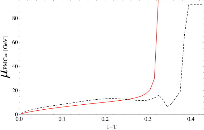
We notice that the two PMC∞ scales have similar behaviors in the range and that the LO-PMC∞ scale agrees with the PMC scale used in Ref. [87]. Small numerical fluctuations are visible in the NLO-PMC∞ scale as unphysical "kinks", due to the Monte-Carlo simulation results of Ref.[174]. In the range , where they are more evident, an interpolation has been performed. However, for the case of thrust, these have a negligible effect on the final distribution and do not depend on the method used for setting the scale, e.g. the PMC∞, but on the method used for performing the calculations (i.e. the Monte-Carlo [174]).
The PMC∞ method totally eliminates both the ambiguity in the choice of the renormalization scale and the scheme dependence to all orders in QCD.
5.2 NNLO thrust distribution results
We use here the results of Ref. [173, 174] and for the running coupling we use the RunDec program [193]. In order to normalize the thrust distribution consistently, we expand the denominator in while the numerator has the couplings renormalized at different PMC∞ scales and . We point out here that the proper normalization would be given by the integration of the total cross-section after renormalization with the PMC∞ scales, nonetheless since the PMC∞ prescription only involves absorption of higher-order terms into the scales, the difference would be within the accuracy of the calculations, i.e. . Equation (5.3) becomes:
| (5.13) |
where the are normalized subsets that are given by:
| (5.14) |
are the scale-invariant conformal coefficients (i.e. the coefficients of each perturbative order not depending on the scale ) while are the couplings determined at the scales respectively.
Normalized subsets for the region can be achieved simply by setting in the Eq. (5.14). Within the numerical precision of these calculations there is no evidence of the presence of spurious terms, such as any further UV-finite term up to NNLO [194], besides the kinematic term at lowest order in the multi-jet region. These terms, if there are any, must remain rather small over the entire range of the thrust variable in comparison with the term or even be compatible with numerical fluctuations. Moreover, we notice a small rather constant difference between the iCF-predicted and the calculated coefficient for the color factor of Ref. [173], which might be due to an UV-finite coefficient or possibly to statistics. This small difference must be included in the conformal coefficient but it has a completely negligible impact on the total thrust distribution.
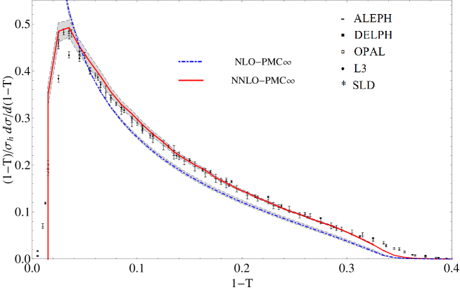
In Fig. 5.2 we show the thrust distribution at NLO and at NNLO with the use of the PMC∞ method. Theoretical errors for the thrust distribution at NLO and at NNLO are also shown (the shaded area). Conformal quantities are not affected by a change of renormalization scale. Thus, the errors shown give an evaluation of the level of conformality achieved up to the order of accuracy and they have been calculated using standard criteria, i.e. varying the remaining initial scale value in the range .
We recall that the distributions are calculated by a Monte-Carlo simulation, considering 50 equidistant bins in the range , thus the peak in the NNLO-PMC∞ distribution appears more as a broken-straight line also due to the linear interpolation used in the figure to join the points.
Using the same definition of the parameter given in Eq. (5.6), we have in the interval an average error of and for the thrust at NLO and at NNLO respectively. A greater improvement has been obtained over the entire range of reliable results for thrust distribution, i.e. , from to from NLO to the NNLO accuracy with the PMC∞.
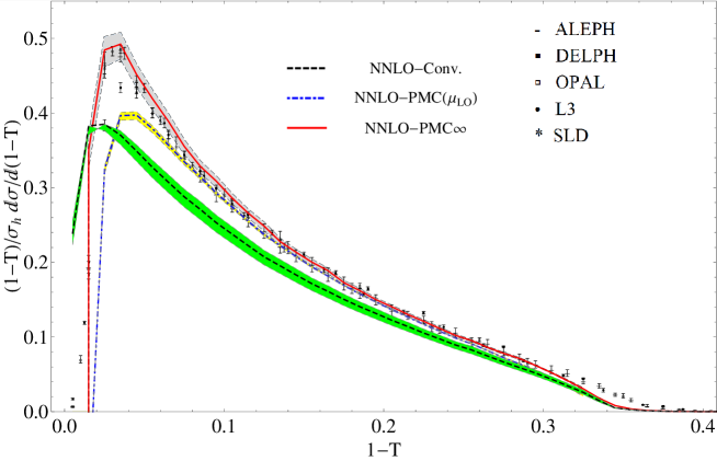
In Fig. 5.3 a direct comparison of the PMC∞ with the CSS results (obtained in [173] and [189, 190]) is shown. In addition, we show the results of the first PMC approach used in [87], which we indicate as PMC(LO) extended to NNLO accuracy. In this approach the last unknown PMC scale NLO of the NLO was set to the last known PMC scale LO of the LO, while the NNLO scale NNLO was left unset and varied in the range .
Average errors calculated in different regions of the spectrum are reported in Table 5.1. The PMC cannot be defined in the range since ; thus the third and fifth row in Table 5.1 are blank. In fact, this further analysis was performed in order to show that the procedure of setting the last unknown scale to the last known one leads to stable and precise results and is consistent with the proper PMC method over a wide range of accessible values of the variable.
| Conv. | PMC(LO) | PMC∞ | |
|---|---|---|---|
| 6.03 | 1.41 | 1.31 | |
| 6.97 | 2.19 | 0.98 | |
| 8.46 | — | 2.61 | |
| 5.34 | 1.33 | 1.77 | |
| 6.00 | — | 1.95 |
From the comparison with the CSS, we notice that the PMC∞ prescription significantly improves the theoretical predictions. Moreover, results are in remarkable agreement with the experimental data over a wider range of values and they show an improvement of the PMC results when the two-jet and multi-jet regions are approached, i.e. the region of the peak and the region respectively. The use of the PMC∞ approach in perturbative QCD thrust calculations restores the correct behavior of the thrust distribution in the region and this is a clear effect of the iCF property. Comparison with experimental data has been improved over the entire spectrum and the introduction of the correction would improve this comparison especially in the multi-jet region. In the PMC∞ method theoretical errors are given by the unknown intrinsic conformal scale of the last order of accuracy. We expect this scale not to be significantly different from that of the previous orders. In this particular case, as shown in Eq. (5.14), we also have a dependence on the initial scale left due to the normalization and to the regularization terms. These errors represent 12.5% and 1.5% respectively of the full theoretical errors in the range and they could be improved by means of a correct normalization.
5.3 NNLO -parameter distribution results
The same analysis applies straightforwardly to the -parameter distribution including the regularizing parameter, which has been set to the same value . The same scales of Eq. (5.7) and Eq. (5.10) apply to the -parameter distribution in the region and in the region . In fact, due to kinematic constraints that set the , we also have the same iCF effect for the -parameter.
Results for the -parameter scales are shown in Fig. 5.4. We notice the effect of the iCF intrinsic conformality on the LO-PMC∞ scale, which terminates at the kinematic boundary . In fact, at this boundary and thus sets the whole conformal subset . The NLO-PMC∞ scale has two distinct domains separated by the kinematic constraint . In the range , the NLO-PMC∞ scale has the same physical behavior as the LO-PMC∞ scale, in the range is almost constant, due to a similar behavior of the numerator and denominator in Eq.5.12 and at it goes through a saturation effect given by the coefficient in Eq.5.12, which becomes null. Results for the -parameter distributions are shown in Fig. 5.5.
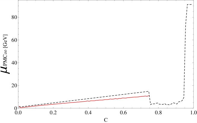
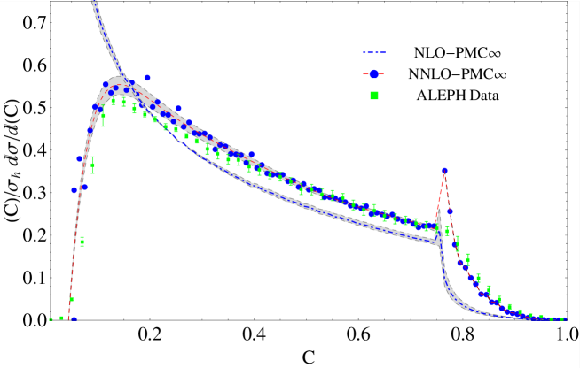
Theoretical errors have been calculated, as in the previous case, using standard criteria and results indicate an average error over the entire spectrum of the -parameter distribution at NLO and at NNLO of and respectively.
| [%] | Conv. | PMC(LO) | PMC∞ |
|---|---|---|---|
| 4.77 | 0.85 | 2.43 | |
| 11.51 | 3.68 | 2.42 | |
| 6.47 | 1.55 | 2.43 |
A comparison of average errors according to the different methods is displayed in Table 5.2. Results show that the PMC∞ improves the NNLO QCD predictions for the -parameter distribution over the entire spectrum.
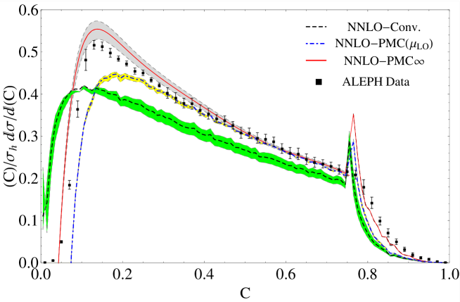
A comparison of the distributions calculated with the CSS, the PMC(LO) [88] and the PMC∞ is shown in Fig. 5.6. The results for the PMC∞ display remarkable agreement with the experimental data away from the regions and . The errors due to the normalization and to the regularization terms (Eq. (5.14)) are respectively and of the full theoretical errors.
The perturbative calculations could be further improved using a correct normalization and also by introducing the resummation of the large-logarithm technique in order to extend the perturbative regime and to eliminate the unphysical spike at , which is due to enhanced logarithmic terms at the kinematic boundary.
5.4 The thrust distribution in the QCD conformal window and in QED
For the first time, we employ the perturbative regime of the quantum chromodynamics (pQCD) infrared conformal window as a laboratory to investigate in a controllable manner (near) conformal properties of physically relevant quantities, such as the thrust distribution in electron–positron annihilation processes [90]. The conformal window of pQCD has a long and noble history conveniently summarized and generalized to arbitrary representations in Ref. [195]. Several lattice gauge theory applications and results have been summarized in a recent report on the subject in Ref. [196].
5.4.1 The thrust distribution according to
It would be highly desirable to compare the PMC and CSS methods along the entire renormalization group flow from the highest energies down to zero energy. This is precluded in standard QCD with a number of active flavors less than six because the theory becomes strongly coupled at low energies. We therefore employ the perturbative regime of the conformal window (Sec. 2.2.2) which allows us to arrive at arbitrary low energies and obtain the corresponding results for the SU() case at the cost of increasing the number of active flavors. Here we are able to deduce the full solution at NNLO in the strong coupling. In this section we shall consider the region of flavors and colors near the upper bound of the conformal window, i.e. , where the IR fixed point can be reliably accessed in perturbation theory and we compare the two renormalization scale setting methods, the CSS and the PMC∞.
Results for the thrust distribution calculated using the NNLO solution for the coupling , at different values of the number of flavors, , is shown in Fig. 5.7.
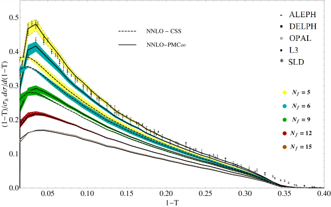
A direct comparison between PMC∞ (solid line) and CSS (dashed line) is shown at different values of the number of flavors. We notice that, despite the phase transition (i.e. the transition from an infrared finite coupling to an infrared divergent coupling), the curves given by the PMC∞ at different , preserve with continuity the same characteristics of the conformal distribution setting outside the conformal window of pQCD.
Technically, this is explained by the fact that the PMC∞ reabsorbs all the terms into the running coupling and the PMC∞ scales are both above 2 GeV in almost the entire range of the distribution; in particular, for values in the range , and thus the PMC∞ thrust distribution is affected by the change of behavior of the coupling only in the first two bins at . However, this region is a multi-scale region and is not only affected by nonperturbative effects, but also by the presence of large-logarithms deriving from incomplete IR cancellation. On the other hand, the CSS distribution is more sensitive to the decreasing of .
In fact, the position of the thrust distribution peak is well preserved varying in and outside the conformal window using the PMC∞, while there is a constant shift towards lower values using the CSS. These trends are shown in Fig. 5.8. We notice that in the central range, , the position of the peak is exactly preserved using the PMC∞ and overlaps with the position of the peak shown by the experimental data. According to our analysis for the case PMC∞, in the range , the number of bins is insufficient to resolve the peak, although the behavior of the curve is consistent with the presence of a peak in the same position, while for , the peak is no longer visible. Theoretical uncertainties on the position of the peak have been calculated using standard criteria, i.e. by varying the remaining initial scale value in the range and considering the lowest uncertainty given by the half the spacing between two adjacent bins.
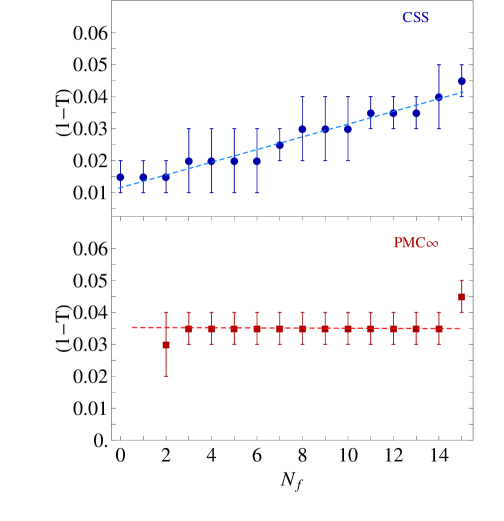
Using the definition given in Eq. (5.6), we have determined the average error, , calculated in the interval of thrust and results for CSS and PMC∞ are shown in Fig. 5.9. We notice that the PMC∞ in the perturbative and IR conformal window, i.e. , which is the region where in the entire range of the renormalization scale values, from up to , the average error given by PMC∞ tends to zero () while the error given by the CSS tends to remain constant (). Comparison of the two methods shows that, outside the conformal window, , the PMC∞ leads to higher precision.
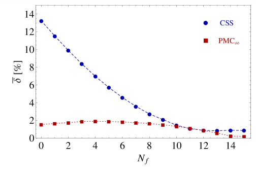
From our analysis in section 2.2.2, it follows that the IR fixed point at is not phenomenologically accessible, assuming a measured value of the coupling at a certain scale, since in the region , the coupling would no longer have the UV asymptotically free behavior. Thus, in order to have a phenomenological application of the Banks-Zaks variable, (i.e. , as shown in Refs.[197, 198]), one should be able to reach any small value of the coupling above the Planck scale in QCD, since the IR fixed point is interacting. Moreover, a conformal result is just characterized by the absence of running of the coupling and not necessarily by a null value. A straight conformal solution of Eqs. 2.31 and 2.32, is given by: , with for any scale . Our application of the Banks-Zaks results shows that the conformal limit of the thrust distribution is less sensitive to the method adopted to set the renormalization scale, CSS or PMC∞, once the same phenomenological value of the coupling has been determined at a certain scale. We suggest that a more suitable variable for the expansion would be given by , where is the maximum allowed value of to be asymptotically free, introduced by the phenomenological value of the coupling at an initial scale .
5.4.2 The thrust distribution in the Abelian limit
We consider now the thrust distribution in U(1) Abelian QED, which rather than being infrared interacting is infrared free. We obtain the QED thrust distribution performing the limit of the QCD thrust at NNLO according to [32, 145]. In the zero number of colors limit the gauge group color factors are fixed by , where is the number of active leptons, while the -terms and the coupling rescale as and respectively. In particular, and using the normalization of Eq. (2.15). According to this rescaling of the color factors, we have determined the QED thrust and the QED PMC∞ scales. For the QED coupling, we have used the analytic formula for the effective fine structure constant in the scheme:
| (5.15) |
with and the vacuum polarization function () calculated perturbatively to two loops, including contributions from leptons, quarks and the boson. The QED PMC∞ scales have the same form of Eqs. (5.7) and (5.10) with the factor for the scheme set to and the regularization parameter introduced to cancel singularities in the NLO PMC∞ scale in the limit tends to the same QCD value, . A direct comparison between QED and QCD PMC∞ scales is shown in Fig. 5.10.
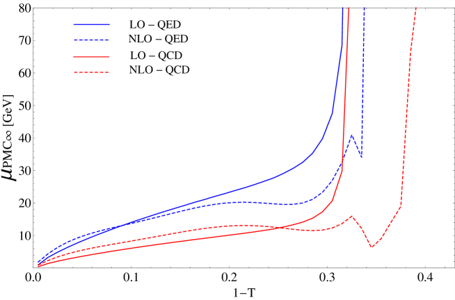
We note that in the QED limit the PMC∞ scales have analogous dynamical behavior to those calculated in QCD; differences arise mainly owing to the scheme factor reabsorption, the effects of the number of colors at NLO are very small. Thus, we notice that perfect consistency is shown from QCD to QED using the PMC∞ method. The normalized QED thrust distribution is shown in Fig. 5.11. We note that the curve is peaked at the origin, , which suggests that the three-jet event in QED occurs with a rather back-to-back symmetry. Results for the CSS and the PMC∞ methods in QED are and show very small differences, given the good convergence of the theory.
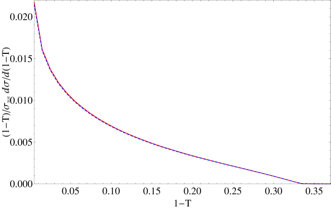
5.5 A novel method for the precise determination of the strong coupling and its behavior
In this section we present a novel method for precisely determining the running QCD coupling constant over a wide range of from event-shape variables for electron–positron annihilation measured at a single center-of-mass energy , based on PMC scale setting. In particular, we display the results obtained in Refs. [88, 87] using the approach of a single PMC scale at LO and NLO, i.e. the PMC(LO) of the previous section.
The precise determination of the strong coupling is one of the crucial tests of QCD. The dependence of on the renormalization scale obtained from many different physical processes shows consistency with QCD predictions and asymptotic freedom. The Particle Data Group (PDG) currently gives the world average: [126] in the renormalization scheme.
Particularly suitable to the determination of the strong coupling is the process jets since its leading order is [176]. Currently, theoretical calculations for event shapes are based on CSS. By using conventional scale setting, only one value of at the scale can be extracted and the main source of the uncertainty is given by the choice of the renormalization scale. Several values for the strong coupling have been extracted from several processes, e.g. [199] is obtained by using perturbative corrections and resummation of the large logarithms in the NNLO+NLL accuracy predictions. Other evaluations improving the resummation calculations up to N3LL give a result of [31] from thrust and [200] from the -parameter. Nonperturbative corrections for hadronization effects have also been included in Ref. [201], but as pointed out in Ref. [202], the systematics of the theoretical uncertainties introduced by hadronization effects are not well understood.
In this section we show that by using the PMC, it is possible to eliminate the renormalization scale ambiguities and obtain consistent results for the strong coupling using the precise experimental data of event-shape variable distributions. We notice that improved event-shape distributions have been obtained in Refs. [44, 194, 203] using BLM and soft and collinear effective theory (SCET).
5.5.1 Running behavior
Given that the PMC scale (PMC(LO)) is not a single-valued but rather a monotonically increasing function of and of the selected observable,(as shown in Figs. 5.1 and 5.4), it is possible to determine the strong coupling at different scales from one single experiment at one single center-of-mass energy. The dependence of the scale on the observable reflects the dynamics of the underlying gluon and quark subprocess. This dynamics also varies the number of active flavors . Considering that PMC scales for QCD and QED show the same behavior and that their relation at LO is only given by a RS redefinition term, , this approach may also be extended to QED.
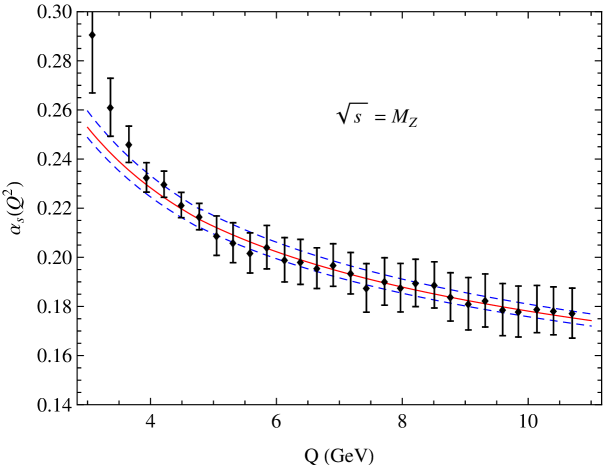
We extract at different scales bin-by-bin from the comparison of PMC predictions for () and differential distributions with measurements at . The extracted values from the -parameter distribution are shown in Fig. 5.12. We note that the values extracted in the scale range of GeV GeV are in excellent agreement with those evaluated from the world average [126]. Given that the PMC scale setting eliminates the scale uncertainties, the corresponding extracted values are not plagued by ambiguities in the choice of . The extracted values from the thrust observable using PMC are shown in Fig. 5.13. There is good agreement also in this case in the range GeV GeV (corresponding to the range ). These extracted values of are also in good agreement with the world average value of the PDG [126].
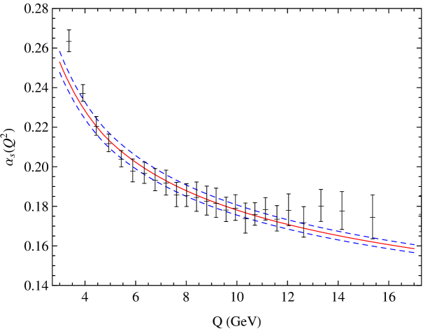
Thus, PMC scale setting provides a remarkable way to verify the running of from event shapes measured at a single energy of . Analogously in QED, the running of the QED coupling can be measured at a single energy of (see e.g. [204]).
The differential distributions of event shapes are afflicted with large logarithms especially in the two-jet region. Thus, the comparison of QCD predictions with experimental data and thus the extracted values are restricted to the region where the theory is able to describe the data well. Choosing a different area of distributions leads to the different values of .
5.5.2 from a fit
In order to obtain a reliable at the scale of the mass, we determine from the fit of the PMC predictions to measurements. In particular, we perform the fit by minimizing the respect to the parameter. The variable is defined as:
where is the value of the experimental data, is the corresponding experimental uncertainty and is the theoretical prediction. The fit for thrust and the -parameter leads to the following results:
| (5.16) | |||||
with d.o.f. for the thrust mean value and
| (5.17) | |||||
with d.o.f. for the -parameter mean value, where the first error is the experimental uncertainty and the second the theoretical uncertainty. Both results are consistent with the world average [126].
The precision of the extracted has been greatly improved by using the PMC: the dominant scale uncertainties are eliminated and the convergence of pQCD series is greatly improved. In particular, a strikingly much faster pQCD convergence is obtained for the mean thrust value [87], theoretical uncertainties are even smaller than the experimental uncertainties. We remark that these results for are among the most precise determinations of the strong coupling at the mass from event-shape variables.
6 Comparison of the PMCm, PMCs and PMC for fully integrated fundamental quantities
In this section, we show predictions for three important quantities: , and , which have been calculated up to four-loop QCD corrections using alternative PMC scale-setting procedures. Numerical results for the conventional, PMCm, PMCs and PMC∞ approaches will be presented. For self-consistency, the same loop -running behavior will be adopted for calculating the same loop perturbative series. The QCD asymptotic scale () is then fixed by using [126] and for a four-loop prediction, we obtain MeV and MeV in a conventional renormalization scheme.
6.1 The pQCD predictions for , and
The annihilation of electrons and positrons into hadrons provides one of the most important platforms for determining the running behavior of the QCD coupling. The ratio is defined as
| (6.1) | |||||
where , corresponding to the electron–positron collision energy in the center-of-mass frame. The pQCD series for , up to -loop QCD corrections, is
The perturbative coefficients in the scheme up to four-loop level have been calculated in Refs. [205, 162, 206, 207]. As a reference point, at GeV, we have [208].
Another useful ratio is for -lepton decays into hadrons, defined as
| (6.2) | |||||
where [126] is the relevant Cabibbo–Kobayashi–Maskawa matrix element, and for the electroweak corrections, for light-quark mass effects666An improved determination of the and from the -decay has been recently shown in Ref. [209]., for the nonperturbative effects and GeV [210, 211, 205]. The pQCD series for up to -loop QCD corrections is
where the perturbative coefficients up to four-loop QCD corrections can be derived by using the relation between and [212].
The decay width for Higgs boson decay into a bottom and anti-bottom pair, , can be written as
| (6.3) |
where the Fermi constant , the Higgs mass GeV and the -quark running mass is GeV [69]. The pQCD series for up to -loop QCD corrections is
The perturbative coefficients up to four-loop QCD corrections have been calculated in Ref. [213]. In the following, we give the properties for the pQCD series of GeV), and using each scale-setting approach. As for the leading-order ratios with , we have no information to set the renormalization scale for all the scale-setting approaches; and for convenience, we directly set it to be , , or , respectively, which gives , and . We point out that all four-loop calculations for these observables derive from analytic properties (of the Adler function) rather than from a direct multi-loop calculation of the perturbative series.
6.2 Properties using the conventional scale-setting approach
We present the perturbative coefficients in Table 6.1, where the errors are evaluated by taking for GeV), for and for , respectively. Table 6.1 shows that those coefficients are highly scale dependent.
We present the results of GeV), and up to four-loop QCD corrections using the conventional scale-setting approach in Table 6.2, where the errors are evaluated by taking for GeV), for and for , respectively. For self-consistency, we adopt the th-loop -running behavior in deriving th-loop prediction for GeV), and . We define the ratio
where stands for , and , respectively. It shows how the “known” prediction is affected by the one-order-higher terms. Table 6.2 shows that generally we have for all those quantities, consistently with the perturbative nature of the series and indicates that one can obtain more precise predictions by including more loop terms. To show the perturbative nature more explicitly, we present the magnitudes of each loop term for the four-loop approximants , and in Table 6.3, which displays the relative importance among the LO, NLO, N2LO and N3LO terms, which for those approximants are
| (6.4) | |||
| (6.5) | |||
| (6.6) |
where the central values are for , and ; and the errors are for , and , respectively. Consistently with Table 6.2, the scale dependence for each loop term is large, but due to the cancellation of scale dependence among different orders, the net scale dependence is small, e.g. , and for GeV), and , respectively. Note that due to the usual renormalon divergence and a larger value at a smaller scale , i.e. , the net scale dependence of the four-loop prediction is still sizable.
In the pQCD calculation, it is helpful to give a reliable prediction of the uncalculated higher-order terms. The Padé approximant approach (PAA) [130, 131, 132], shown in Eq. (2.38), provides an effective method to estimate the th-order coefficient from a given -th-order series.777Another method, which uses the scale-invariant conformal series together with the Bayesian model [214, 215, 216] to provide probabilistic estimates of the unknown higher-orders terms has been proposed [217] In practice, it has been found that the PAA becomes more effective when more loop terms are known. For a pQCD approximant, , the predicted N3LO and the N4LO terms are
| (6.7) | |||||
| (6.8) | |||||
| (6.9) | |||||
| (6.10) | |||||
| (6.11) |
| : | : | |
| — | : | |
| : | : | |
| — | : | |
| : | : | |
| — | : |
Table 6.4 displays the preferable diagonal-type PAA predictions [133] of the and terms of GeV), and using the conventional scale-setting approach. Owing to the large scale dependence of each loop term, the PAA predictions show large scale dependence. The two allowable diagonal-type PAA predictions for terms are consistent with each order within errors. Comparing Table 6.4 with Table 6.3, we note that the values of the predicted terms agree with their exact values within errors. Thus, by employing a perturbative series with enough higher-order terms, the PAA prediction can be made reliable.
6.3 Properties using the PMCm approach
Following the standard PMCm procedures, the nonconformal -terms are eliminated by using the RGE recursively, determining the effective at each perturbative order and resulting in the renormalon-free and scheme-independent conformal series (3.14).
We present the conformal coefficients in Table 6.5. The PMC scales are of a perturbative nature, which leads to the first kind of residual scale dependence for PMCm predictions. If the pQCD approximants are known up to four-loop QCD corrections, three PMC scales (, and ) can be determined up to , and order, which are 41.19, 36.85, 168.68 GeV for GeV), 1.26, 0.98, 0.36 GeV for and 62.03, 40.76, 52.76 GeV for , accordingly. There is no -term to set the scale , the PMCm prediction has the second kind of residual scale dependence. As mentioned in Sec. 3.1, there is the second kind of residual scale dependence for PMCm series and, for convenience, we set as the default choice of . A discussion of the magnitude of the second kind of residual scale dependence by taking some other typical choices of will be presented at the end of this subsection. For the scales , we adopt the usual approximate four-loop analytic solution of the RGE to derive the value of . Due to the sizable difference between the approximate analytic solution and the exact numerical solution of the RGE at scales below a few GeV [52, 126], we adopt the exact numerical solution of the RGE to evaluate at 1.26 GeV and 0.98 GeV. For the scales close to , various low-energy models have been suggested in the literature; a detailed comparison of various low-energy models can be found in Ref. [99]. For definiteness, we shall adopt the Massive Perturbation Theory (MPT) model [218] to evaluate at GeV, which gives , where is the parameter in the MPT model.
We present the results of GeV), and up to four-loop QCD corrections using the PMCm scale-setting approach in Table 6.6. Table 6.6 shows that the PMCm predictions generally have behavior close to the central predictions under conventional scale-setting procedures, especially when more loop terms are known. This is due to the fact that when the renormalization scale of the conventional series is set as the one to eliminate the large logarithms, the divergent renormalon terms may also be simultaneously removed, since the -terms are always accompanied by the logarithm terms.
We present the value of each loop term for the four-loop predictions GeV), and using the PMCm scale-setting approach in Table 6.7.888By using the RGE recursively, one can obtain correct value and achieve good matching of to its coefficients at the same perturbative order. However, such treatment is a sort of -resummation and the resultant PMC series is no longer the usual fixed-order series. Thus, the function of Table 6.7 is to show its own perturbative behavior. The relative importance among the LO terms, the NLO terms, the N2LO terms and the N3LO terms for those approximants are
| (6.12) | |||
| (6.13) | |||
| (6.14) |
Table 6.7 shows that there are residual scale dependences of GeV) and for the LO and NLO terms that are quite small (e.g. the errors are only about of the LO terms and of the NLO terms, respectively), which are smaller than the corresponding ones under the conventional scale-setting approach. However, the residual scale dependence of is sizable – approximately – and is comparable to the conventional scale dependence. Here the large residual scale dependence of is reasonable, caused by the poor pQCD convergence for the PMC scales at higher orders and the uncertainties of the -running behavior in the low-energy region.
As a final remark, we discuss the possible magnitudes of the second kind of residual scale dependence under the PMCm scale-setting approach by taking some other typical choices of , e.g. , , , and , which also ensures the scheme independence of the PMCm series. Table 6.8 shows that the second kind of residual scale dependence of , and are , and , respectively. It shows that those choices will change the magnitudes of , and at the default choice of by about , and , respectively. For , another uncertainty caused by the MPT model parameter is in the choice of . We also give the numerical results under some other choices of the undetermined in Table 6.8. It shows that the MPT model parameter will lead to uncertainties. These uncertainties caused by the small scale and undetermined scale indicate that we still need a more appropriate scale-setting approach to suppress the theoretical uncertainties.
6.4 Properties using the PMCs approach
The PMCs approach provides a method to suppress the residual scale dependence. Applying the standard PMCs scale-setting procedures, we obtain an overall effective and, accordingly, an overall effective scale () for GeV), and , respectively. If they are known up to two-loop, three-loop and four-loop levels, the PMC scale can be determined up to , and accuracies, respectively. That is, for , we have
| (6.15) | |||||
| (6.16) | |||||
| (6.17) |
Their magnitudes become more precise as one includes more loop terms and the difference between the two nearby values becomes smaller and smaller when more loop terms are included, e.g. the scales only shift by about to the ones. Since these PMCs scales are numerically sizable, one avoids confronting the possibly small scale problem at certain perturbative orders of the multi-scale-setting approaches, such as PMCm, PMC∞.
We present the results of GeV), and up to four-loop QCD corrections using the PMCs scale-setting approach in Table 6.9. We also present the value of each loop term for the four-loop approximants GeV), and using the PMCs scale-setting approach in Table 6.10. The relative importance among the LO terms, the NLO terms, the N2LO terms and the N3LO terms for those approximants are
| (6.18) | |||
| (6.19) | |||
| (6.20) |
These are comparable to the convergent behavior of the PMCm series and are more convergent than conventional predictions. Moreover, the sizable residual scale dependence of appearing in Table 6.7 has been eliminated by using the PMCs procedure. Thus, the PMCs approach, which requires a much simpler analysis, can be adopted as a reliable substitute for the basic PMCm approach to setting the renormalization scales for high-energy processes, with small residual scale dependence. As a conservative estimate of the first kind of residual scale dependence, we take the magnitude of its last known term as the unknown N3LL term, e.g. for GeV), and . We then obtain
| (6.21) | |||||
| (6.22) | |||||
| (6.23) |
which show that the first kind of residual scale dependence is about , and .999Since the N2LL accuracy -series of these pQCD approximants already show good perturbative behavior, it is found that by using the PAA predicted N3LL term, e.g. , to perform the estimates, one can obtain smaller first kind of residual scale dependence than the ones listed in Eqs. (6.21), 6.22, 6.23), which are , and , respectively. More explicitly, we show the conservative estimate of the first kind of residual scale dependence under the PMCs in Figs. 6.1, (6.2) and (6.3), respectively.
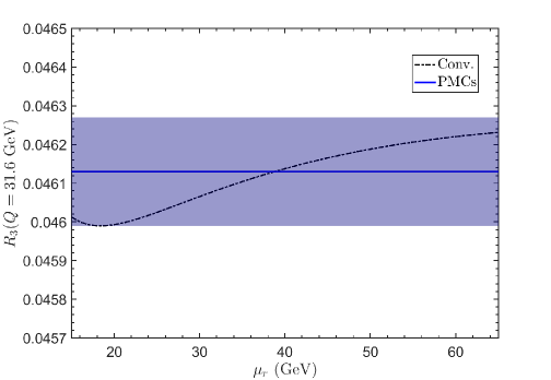
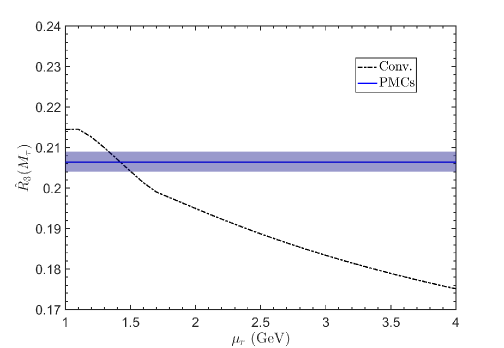
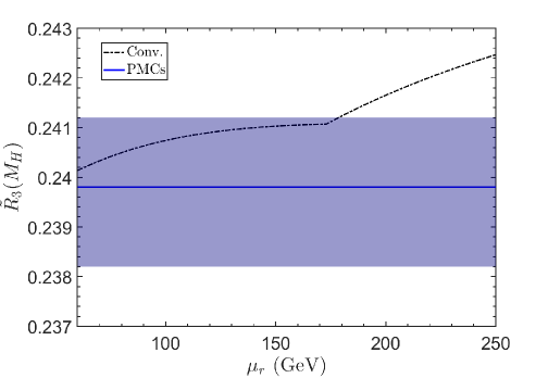
The conformal PMCs series is scheme and scale independent; it thus provides a reliable basis for estimating the effect of unknown higher-order contributions. At present, there is no way to use a series with different effective at different orders; and if there were any, its effectiveness would also be greatly affected by the possibly large residual scale dependence. Thus, we shall not use PMCm, PMC∞ series to estimate the contribution of the unknown terms. As for the PMCs series, with an overall effective , we may directly use the PAA [219].
| [0/2]: | [0/3]: | |
| [0/2]: | [0/3]: | |
| [0/2]: | [0/3]: |
| [0/2]: | [0/3]: | |
| [0/2]: | [0/3]: | |
| [0/2]: | [0/3]: |
We present the preferable []-type PAA predictions for the PMCs series of GeV), and in Table 6.11 and 6.12. Table 6.11 shows the predicted and conformal coefficients and . Note that the predicted values are close to the exact values shown in Table 6.5 and those known conformal coefficients do not change when more loop terms are known. To obtain the final numerical result, we need to combine the coefficients and with the effective at corresponding orders. Table 6.12 displays the numerical results, these values will be very slightly changed for a more accurate , since the accuracy is already changed from that at by less than .
6.5 Properties using the PMC∞ approach
Given the unique form of intrinsic conformality iCF, any other attempt (such as PMCa [107]) to write the perturbative expansion in a scale-invariant form would lead to the iCF (as shown in Ref. [62]).
Following the standard PMC∞ procedures, we calculate GeV), and up to four-loop QCD corrections. The perturbative coefficients () are exactly the same as those of the PMCm and PMCs conformal coefficients (). As shown by Eqs. (4.12), (4.14), (4.15), the PMC∞ scales are definite and have no perturbative nature, they are free of renormalization scale ambiguities and do not have the first kind of residual scale dependence. Using the four-loop QCD corrections, we can determine their first three scales, i.e.
| (6.24) | |||||
| (6.25) | |||||
| (6.26) |
For the case GeV), its third scale GeV is quite small and we adopt the above-mentioned MPT model to estimate its contribution, which gives . As mentioned in Sec. 4, the fourth scale is fixed to the initial scale , i.e. the kinematic scale of the process, and varied in the range to ascertain the level of conformality achieved by the series. In fact, the last PMC scale is entangled with the missing higher-order contributions. This is referred as second kind of residual scale dependence.
We present the results of GeV), and up to four-loop QCD corrections using the PMC∞ scale-setting approach in Table 6.13. For the cases GeV) and , we have , indicating that the second kind of residual scale dependence is sizable for these two quantities, which largely affects the magnitude of the lower-order series. When one has enough higher-order terms, the residual scale dependence is highly suppressed owing to the more convergent renormalon-free series. For example, we present the value of each loop term (LO, NLO, N2LO or N3LO) for the four-loop predictions GeV), and in Table 6.14. At the four-loop level, the PMC∞ series already exhibits convergent behavior. As shown in Table 6.14, the relative importance among the LO terms, the NLO terms, the N2LO terms and the N3LO terms for those approximants are
| (6.27) | |||
| (6.28) | |||
| (6.29) |
This perturbative behavior is similar to the predictions of PMCm and PMCs, except for GeV), which due to a much smaller scale leads to quite large N2LO terms.
6.6 A comparison of the renormalization scale dependence of the various PMC approaches
We present the renormalization scale () dependence of the four-loop predictions GeV), and using the conventional, PMCm, PMCs and PMC∞ scale-setting procedures in Figs. 6.4, 6.5 and 6.6, respectively. In these figures, we show the second kind of residual scale dependence of GeV), under the PMCm and PMC∞ scale-setting procedures with the shaded bands. The green/lighter bands are obtained by changing the undetermined to , , , and . And the red/darker bands are obtained by varying the undetermined PMC∞ scale within the range for GeV), for and for .
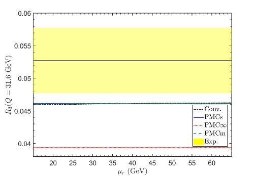
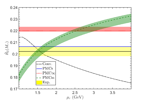
Figure 6.4 shows that the theoretical predictions are smaller than the experimental result. This is reasonable since we have adopted the world average [126] to set for all these observables and, if we adopt a strong coupling fixed by using the annihilation data alone, we obtain consistent predictions in agreement with the data. For example, using [199], fixed by using the hadronic event shapes in annihilation to set , we obtain a larger GeV), e.g. for the PMCs approach, which is consistent with within errors. It has been noticed that the second kind of residual scale dependence of GeV) under the PMCm and PMC∞ scale-setting procedure are both very small, since the order correction is highly suppressed in GeV). These figures show that by including enough higher-order terms, the following hold.
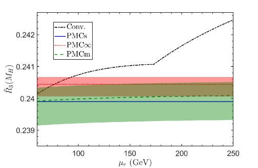
-
1.
The renormalization scale dependence of the conventional prediction depends strongly on the convergence of the perturbative series and the cancellation of scale dependence among different orders. For a numerically strongly convergent series, such as GeV) and , the net scale dependence is only parts per thousand for a wide range of scale choices. For a less convergent series, such as , the net renormalization scale uncertainty is sizable, which is up to for , for and for ;
-
2.
The PMCm predictions have two kinds of residual scale dependence due to unknown terms. The second residual scale dependence can be greatly suppressed by the extra requirement of conformal invariance; the first property then dominates the net residual scale dependence. For numerically convergent series, such as GeV) and , the residual scale dependences are small, i.e. less than four parts per thousand.101010As a comparison, the conventional scale dependence of is about nine parts per thousand for For a less convergent series, such as , due to the large residual scale dependence of the NLO terms, its net residual scale dependence is sizable, it is for , for and for . Although in some special cases, such as , the residual scale dependence may be comparable to the conventional prediction, the PMCm series has no renormalon divergence and it generally has a better pQCD convergence. For the case of GeV) and , the PMCm predictions show weaker dependence on and its prediction can be more accurate than conventional pQCD predictions;
-
3.
The PMC∞ predictions only have the second kind of residual scale dependence, which are suppressed for the present four-loop predictions. The magnitude of the residual scale dependence depends on the convergence of the resultant series and for the present processes, the second kind of residual scale dependence are only about parts per thousand to a few percent. Due to the application of “intrinsic conformality” or equivalently the requirement of scale invariance at each order, the PMC∞ scales determined are not of a perturbative nature, but they can be very small in certain cases. For the case GeV), we obtain a much smaller scale GeV, which is unreasonable and indicates that the PMC∞ approach may not be applicable for this process. To obtain a numerical estimate, we have adopted the MPT model to calculate the magnitude of at such a small scale; Fig. 6.4 shows that the MPT prediction deviates from other approaches by about . By including the uncertainty from the MPT model parameter , the prediction still deviates from other approaches by about ;
-
4.
The PMCs predictions for the dependence of observables on the renormalization scale are flat lines. The first kind of residual scale dependence of the PMCs predictions only affects the precision of the magnitude of effective and the PMCs predictions are exactly independent of the choice of at any fixed order.
7 Summary
The Principle of Maximum Conformality (PMC) provides a rigorous first-principles method to eliminate conventional renormalization scheme and scale ambiguities for high-momentum-transfer processes. Its predictions have a solid theoretical foundation, satisfying renormalization group invariance and all other self-consistency conditions derived from the renormalization group. The PMC has now been successfully applied to many high-energy processes.
In this review, we have presented a new scale-setting procedure, namely PMC∞, which stems from the general PMC and preserves a particular property that we have defined as intrinsic conformality (iCF). The iCF is a particular parametrization of the perturbative series that exactly preserves the scale invariance of an observable perturbatively. We point out that this is a unique property of the perturbative expansion, any other attempt (such as PMCa [107]) to write the perturbative expansion in a scale-invariant form would lead to the iCF (as shown in Ref. [62]).
The PMC∞ solves the conventional renormalization scale ambiguity in QCD, it preserves not only the iCF but also all the features of the PMC approach and leads to a final conformal series at any order of the perturbative calculation. In fact, the final series is given by perturbative conformal coefficients with the couplings determined at conformal renormalization scales. The PMC∞ scale setting agrees with the Gell-Man–Low scheme and can be considered the non-Abelian analog of Serber–Uehling [221, 222] scale setting, which is essential in precision tests of QED and atomic physics.
Given the iCF form, a new “How-To” method for identifying conformal coefficients and scale has been developed and can be applied to either numerical or analytical calculations. The PMC∞ has been applied to the NNLO thrust and -parameter distributions and the results show perfect agreement with the experimental data.
The evaluation of theoretical errors using standard criteria demonstrate that the PMC∞ significantly improves the theoretical predictions over the entire spectra of the shape variables order-by-order and both the IR conformal and QED limits of thrust respect the theoretical consistency requirements. Moreover, the position of the thrust peak is in perfect agreement with experiment and is preserved on varying . Hence, even though for the thrust distribution the peak stems directly from resummation (or partial resummation) of the large logarithms in the low-momentum region, its correct position is fixed by the PMC scale and can be considered a “conformal” property, given its independence from the or terms.
Unlike the previous BLM/PMC approaches, the PMC∞ scales are not perturbatively calculated but are conformal functions of the physical scale(s) of the process and any other unintegrated momentum or variable, e.g. the event-shape variable or . The PMC∞ is totally independent of the initial scale used for renormalization in perturbative calculations and it preserves the scale invariance at all stages of calculation, independently of the kinematic boundary conditions, of the starting order of the observable or of the order of the truncated expansion. Moreover, this property leads to the possibility of determining the entire coupling from a single experiment at a single center-of-mass energy (this new method is in progress and will soon appear.)
The iCF improves the general BLM/PMC procedure and point “3” of Section 3. In the same section, we suggested that an improvement and simplification of the perturbatively calculated BLM/PMC scales, would be achieved by setting the renormalization scale directly to the physical scale of the process, before applying the BLM/PMC procedure. This would remove the initial scale dependence from the perturbatively calculated BLM/PMC scales.
We stress that, in contrast with the other PMCm and PMCs approaches, the PMC∞ preserves the iCF; scales are thus set straightforwardly in kinematic regions where constraints cancel the effects of the lower-order conformal coefficients. These effects are particularly visible in the case of event-shape variables in the multi-jet region. For this case we have shown only fixed-order calculation results and other effects due to factorization, such as large logarithms coming from soft and collinear configurations, have not been included. The iCF effects in these kinematic regions are neglected by the PMCm and PMCs approach, unless an ad hoc prescription is introduced.
Another application of the PMC∞ is presented in Ref. [72] and shows an improvement of the results on with respect to the CSS also in this process. From the detailed comparison shown in Sec. 6, it follows that, though the application of the PMC∞ improves the theoretical predictions also for the , , with respect to the CSS, the PMCs leads to more stable results for these quantities.
In general:
-
The PMCs approach determines an overall effective by eliminating all the RG-dependent nonconformal -terms; this results in a single effective scale which effectively replaces the individual PMC scales of PMCm approach in the sense of a mean-value theorem. The PMCs prediction is renormalization scale-and-scheme independent up to any fixed order. The first kind of residual scale dependence is highly suppressed, since the PMC scale at all known orders is determined at the same highest-order accuracy. There is no second kind of residual scale dependence. The PMCs prediction also avoids the small-scale problem, which sometimes emerges in multi-scale approaches.
-
The PMC∞ approach fixes the PMC scales at each order by using the property of intrinsic conformality, which ensures scale invariance of the pQCD series at each order. The resulting PMC scales have no ambiguities, are not of a perturbative nature and thus avoid the first kind of residual scale dependence. Since the last effective scale of the highest-order perturbative term is set to the kinematic scale or physical scale of the process, the PMC∞ prediction still has a reduced second kind of residual scale dependence. However, when more loop terms are included and scales are not in the nonperturbative regime, all PMC’s lead to similar results.
The PMCs approach is close to the PMCm approach in achieving the goals of the PMC by inheriting most of the features of the PMCm approach. It works remarkably well with fully integrated quantities, but has some difficulties in application to differential distributions, besides the fact that this approach may have an effect of averaging the differences of the PMC∞ scales arising at each order, which might be significant to achieve a given precision at a certain level of accuracy. However, given the small differences that we have found in the first two consecutive PMC∞ scales for thrust and -parameter, i.e. , in the LO allowed kinematic region, i.e. and in , we may argue that in the same accessible kinematic domain two consecutive PMC∞ scales have such small differences that a single-scale approach, such as the PMCs, would be justified, leading to analogously precise predictions.
We recall that only the terms related to the UV-divergent diagrams (i.e. the terms) must be reabsorbed into the PMC∞ scales. Thus, PMC∞ perfectly agrees with the PMCm when an observable has a manifestly iCF form. We remark that the iCF underlies scale invariance perturbatively, i.e. the ordered scale invariance. We also remark that PMC∞ agrees with the single-scale approach PMCs in the case of an observable with a particular iCF form with all scales equal, i.e. . In this sense, the PMCm and PMCs may be considered more as “optimization procedures” that follow the purpose of the maximal conformal series by transforming the original perturbative series into an iCF-like final series by using the PMC scales. In contrast, the PMC∞ does not indicate any particular value of the renormalization scale to be used, but indicates the final limit obtained by each conformal subset and then by the perturbative expansion, once all the terms related to each conformal subset are resummed.
The PMC∞ is RG invariant at each order of accuracy, which means we may perform a change of scale at any stage and reobtain the initial perturbative quantity. In this sense PMC∞ is not to be understood as an “optimization procedure”, but as an explicit RG-invariant form to parametrize a perturbative quantity that leads to the conformal limit faster. By setting the renormalization scale of each subset to the corresponding PMC∞ scale, one simply cancels the infinite series of terms, leading to the same conformal result as the original series. Given that both scales and coefficients are conformal in the PMC∞, the scheme and scale dependence is also completely removed in the perturbative series up to infinity.
It was pointed out in Sec. 6 that the PMC∞ scale might become quite small at a certain order for the case of fully integrated quantities, whose calculations were carried out using the analyticity property of the Adler function (this seems not to occur in direct multi-loop calculations, e.g. for the shape variables); and that the PMC∞ retains the second kind of scale dependence. We stress that the last scale in the PMC∞ controls the level of convergence and the conformality of the perturbative series and is thus entangled with the theoretical error of a given prediction. According to the PMC∞ procedure the last scale must be set to the invariant physical scale of the process, given by . In this review we have shown that the usual PMC practice of setting the last scale equal to the last unknown scale is also consistent for the PMC∞ and leads to precise and stable results. Improvements to these points are currently under investigation.
We finally remark that the evaluation of the theoretical errors using standard criteria shows that the PMC∞ significantly improves the precision of pQCD calculations and eliminates the scheme and scale ambiguities. An improved and more reliable analysis of theoretical errors might be obtained by using a statistical approach for evaluating the contributions of the uncalculated higher-order terms, as suggested in Refs. [214, 215, 216] and recently applied with the PMCs in Refs. [81, 217]. This implementation would lead to a more rigorous method to evaluate errors, also giving indications on the possible range of values for the last unknown PMC∞ scale.
Acknowledgements
We thank Francesco Sannino, André Hoang for useful discussions. XGW is supported in part by the Natural Science Foundation of China under Grant No.12175025 and No.12147102. SQW is supported in part by the Natural Science Foundation of China under Grant No.12265011. SJB is supported in part by the Department of Energy Contract No. DE-AC02-76SF00515. SLAC-PUB-17737.
References
- [1] E. C. G. Stueckelberg de Breidenbach, A. Petermann, Normalization of constants in the quanta theory, Helv. Phys. Acta 26 (1953) 499–520. doi:10.5169/seals-112426.
- [2] M. Gell-Mann, F. E. Low, Quantum electrodynamics at small distances, Phys. Rev. 95 (1954) 1300–1312. doi:10.1103/PhysRev.95.1300.
- [3] A. Peterman, Renormalization Group and the Deep Structure of the Proton, Phys. Rept. 53 (1979) 157. doi:10.1016/0370-1573(79)90014-0.
- [4] C. G. Callan, Jr., Broken scale invariance in scalar field theory, Phys. Rev. D 2 (1970) 1541–1547. doi:10.1103/PhysRevD.2.1541.
- [5] K. Symanzik, Small distance behavior analysis and Wilson expansion, Commun. Math. Phys. 23 (1971) 49–86. doi:10.1007/BF01877596.
- [6] W. Celmaster, R. J. Gonsalves, The Renormalization Prescription Dependence of the QCD Coupling Constant, Phys. Rev. D 20 (1979) 1420. doi:10.1103/PhysRevD.20.1420.
- [7] A. J. Buras, Asymptotic Freedom in Deep Inelastic Processes in the Leading Order and Beyond, Rev. Mod. Phys. 52 (1980) 199. doi:10.1103/RevModPhys.52.199.
- [8] P. M. Stevenson, Resolution of the Renormalization Scheme Ambiguity in Perturbative QCD, Phys. Lett. B 100 (1981) 61–64. doi:10.1016/0370-2693(81)90287-2.
- [9] P. M. Stevenson, Optimized Perturbation Theory, Phys. Rev. D 23 (1981) 2916. doi:10.1103/PhysRevD.23.2916.
- [10] P. M. Stevenson, Optimization and the Ultimate Convergence of QCD Perturbation Theory, Nucl. Phys. B 231 (1984) 65–90. doi:10.1016/0550-3213(84)90307-9.
- [11] P. Stevenson, Sense and Nonsense in the Renormalization Scheme Dependence Problem, Nucl. Phys. B 203 (1982) 472–492. doi:10.1016/0550-3213(82)90325-X.
- [12] G. Grunberg, Renormalization Group Improved Perturbative QCD, Phys. Lett. B 95 (1980) 70, [Erratum: Phys.Lett.B 110, 501 (1982)]. doi:10.1016/0370-2693(80)90402-5.
- [13] G. Grunberg, Renormalization Scheme Independent QCD and QED: The Method of Effective Charges, Phys. Rev. D 29 (1984) 2315–2338. doi:10.1103/PhysRevD.29.2315.
- [14] G. Grunberg, On Some Ambiguities in the Method of Effective Charges, Phys. Rev. D 40 (1989) 680. doi:10.1103/PhysRevD.40.680.
- [15] S. J. Brodsky, G. P. Lepage, P. B. Mackenzie, On the Elimination of Scale Ambiguities in Perturbative Quantum Chromodynamics, Phys. Rev. D 28 (1983) 228. doi:10.1103/PhysRevD.28.228.
- [16] F. Chishtie, D. G. C. McKeon, T. N. Sherry, Renormalization Scheme Dependence in a QCD Cross Section, Phys. Rev. D 94 (5) (2016) 054031. arXiv:1512.08173, doi:10.1103/PhysRevD.94.054031.
- [17] F. A. Chishtie, D. G. C. McKeon, Renormalization Scheme Dependence and the Renormalization Group Beta Function, Phys. Rev. D 95 (11) (2017) 116013. arXiv:1612.01455, doi:10.1103/PhysRevD.95.116013.
- [18] L. F. Abbott, Choosing an Expansion Parameter for QCD, Phys. Rev. Lett. 44 (1980) 1569. doi:10.1103/PhysRevLett.44.1569.
- [19] C. Anastasiou, C. Duhr, F. Dulat, E. Furlan, T. Gehrmann, F. Herzog, A. Lazopoulos, B. Mistlberger, High precision determination of the gluon fusion Higgs boson cross-section at the LHC, JHEP 05 (2016) 058. arXiv:1602.00695, doi:10.1007/JHEP05(2016)058.
- [20] S. Catani, S. Devoto, M. Grazzini, S. Kallweit, J. Mazzitelli, Bottom-quark production at hadron colliders: fully differential predictions in NNLO QCD, JHEP 03 (2021) 029. arXiv:2010.11906, doi:10.1007/JHEP03(2021)029.
- [21] D. J. Gross, A. Neveu, Dynamical Symmetry Breaking in Asymptotically Free Field Theories, Phys. Rev. D 10 (1974) 3235. doi:10.1103/PhysRevD.10.3235.
- [22] B. E. Lautrup, On High Order Estimates in QED, Phys. Lett. B 69 (1977) 109–111. doi:10.1016/0370-2693(77)90145-9.
- [23] M. Beneke, Renormalons, Phys. Rept. 317 (1999) 1–142. arXiv:hep-ph/9807443, doi:10.1016/S0370-1573(98)00130-6.
- [24] C. F. Berger, Z. Bern, L. J. Dixon, F. Febres Cordero, D. Forde, T. Gleisberg, H. Ita, D. A. Kosower, D. Maitre, Next-to-Leading Order QCD Predictions for W+3-Jet Distributions at Hadron Colliders, Phys. Rev. D 80 (2009) 074036. arXiv:0907.1984, doi:10.1103/PhysRevD.80.074036.
- [25] S. Catani, G. Turnock, B. R. Webber, L. Trentadue, Thrust distribution in e+ e- annihilation, Phys. Lett. B 263 (1991) 491–497. doi:10.1016/0370-2693(91)90494-B.
- [26] S. Catani, L. Trentadue, G. Turnock, B. R. Webber, Resummation of large logarithms in e+ e- event shape distributions, Nucl. Phys. B 407 (1993) 3–42. doi:10.1016/0550-3213(93)90271-P.
- [27] S. Catani, M. L. Mangano, P. Nason, L. Trentadue, The Resummation of soft gluons in hadronic collisions, Nucl. Phys. B 478 (1996) 273–310. arXiv:hep-ph/9604351, doi:10.1016/0550-3213(96)00399-9.
- [28] U. Aglietti, L. Di Giustino, G. Ferrera, L. Trentadue, Resummed Mass Distribution for Jets Initiated by Massive Quarks, Phys. Lett. B 651 (2007) 275–292. arXiv:hep-ph/0612073, doi:10.1016/j.physletb.2007.06.034.
- [29] L. Di Giustino, G. Ricciardi, L. Trentadue, Minimal prescription corrected spectra in heavy quark decays, Phys. Rev. D 84 (2011) 034017. arXiv:1102.0331, doi:10.1103/PhysRevD.84.034017.
- [30] A. Banfi, H. McAslan, P. F. Monni, G. Zanderighi, A general method for the resummation of event-shape distributions in annihilation, JHEP 05 (2015) 102. arXiv:1412.2126, doi:10.1007/JHEP05(2015)102.
- [31] R. Abbate, M. Fickinger, A. H. Hoang, V. Mateu, I. W. Stewart, Thrust at with Power Corrections and a Precision Global Fit for , Phys. Rev. D 83 (2011) 074021. arXiv:1006.3080, doi:10.1103/PhysRevD.83.074021.
- [32] S. J. Brodsky, P. Huet, Aspects of SU(N(c)) gauge theories in the limit of small number of colors, Phys. Lett. B 417 (1998) 145–153. arXiv:hep-ph/9707543, doi:10.1016/S0370-2693(97)01209-4.
- [33] A. L. Kataev, Riemann - terms in perturbative QED series, conformal symmetry and the analogies with structures of multiloop effects in N=4 supersymmetric Yang-Mills theory, Phys. Lett. B 691 (2010) 82–86. arXiv:1005.2058, doi:10.1016/j.physletb.2010.06.005.
-
[34]
A. De Rújula, H. Georgi, H. David Politzer,
Demythification
of electroproduction local duality and precocious scaling, Annals of Physics
103 (2) (1977) 315–353.
doi:https://doi.org/10.1016/S0003-4916(97)90003-8.
URL https://www.sciencedirect.com/science/article/pii/S0003491697900038 - [35] W. A. Bardeen, A. J. Buras, D. W. Duke, T. Muta, Deep Inelastic Scattering Beyond the Leading Order in Asymptotically Free Gauge Theories, Phys. Rev. D 18 (1978) 3998. doi:10.1103/PhysRevD.18.3998.
- [36] W. Celmaster, R. J. Gonsalves, QCD Perturbation Expansions in a Coupling Constant Renormalized by Momentum Space Subtraction, Phys. Rev. Lett. 42 (1979) 1435. doi:10.1103/PhysRevLett.42.1435.
- [37] G. ’t Hooft, M. J. G. Veltman, Regularization and Renormalization of Gauge Fields, Nucl. Phys. B 44 (1972) 189–213. doi:10.1016/0550-3213(72)90279-9.
- [38] J. Zeng, X.-G. Wu, X.-C. Zheng, J.-M. Shen, Gauge dependence of the perturbative QCD predictions under the momentum space subtraction scheme, Chin. Phys. C 44 (11) (2020) 113102. arXiv:2004.12068, doi:10.1088/1674-1137/abae4e.
- [39] S. J. Brodsky, X.-G. Wu, Self-Consistency Requirements of the Renormalization Group for Setting the Renormalization Scale, Phys. Rev. D 86 (2012) 054018. arXiv:1208.0700, doi:10.1103/PhysRevD.86.054018.
- [40] X.-G. Wu, S. J. Brodsky, M. Mojaza, The Renormalization Scale-Setting Problem in QCD, Prog. Part. Nucl. Phys. 72 (2013) 44–98. arXiv:1302.0599, doi:10.1016/j.ppnp.2013.06.001.
- [41] A. Dhar, V. Gupta, A New Perturbative Approach to Renormalizable Field Theories, Phys. Rev. D 29 (1984) 2822. doi:10.1103/PhysRevD.29.2822.
- [42] V. Gupta, D. V. Shirkov, O. V. Tarasov, New perturbative approach to general renormalizable quantum field theories, Int. J. Mod. Phys. A 6 (1991) 3381–3397. doi:10.1142/S0217751X91001647.
- [43] A. Deur, S. J. Brodsky, G. F. de Teramond, The QCD Running Coupling, Nucl. Phys. 90 (2016) 1. arXiv:1604.08082, doi:10.1016/j.ppnp.2016.04.003.
- [44] G. Kramer, B. Lampe, Jet production rates at LEP and the scale of alpha-s, Z. Phys. A 339 (1991) 189–193. doi:10.1007/BF01282948.
- [45] S. J. Brodsky, L. Di Giustino, Setting the Renormalization Scale in QCD: The Principle of Maximum Conformality, Phys. Rev. D 86 (2012) 085026. arXiv:1107.0338, doi:10.1103/PhysRevD.86.085026.
- [46] S. J. Brodsky, X.-G. Wu, Scale Setting Using the Extended Renormalization Group and the Principle of Maximum Conformality: the QCD Coupling Constant at Four Loops, Phys. Rev. D 85 (2012) 034038, [Erratum: Phys.Rev.D 86, 079903 (2012)]. arXiv:1111.6175, doi:10.1103/PhysRevD.85.034038.
- [47] S. J. Brodsky, X.-G. Wu, Eliminating the Renormalization Scale Ambiguity for Top-Pair Production Using the Principle of Maximum Conformality, Phys. Rev. Lett. 109 (2012) 042002. arXiv:1203.5312, doi:10.1103/PhysRevLett.109.042002.
- [48] L. Di Giustino, The Renormalization Scale Setting Problem in QCD [Ph.D. Thesis], Ph.D. thesis, Insubria U., Como (2022). arXiv:2205.03689.
- [49] M. Mojaza, S. J. Brodsky, X.-G. Wu, Systematic All-Orders Method to Eliminate Renormalization-Scale and Scheme Ambiguities in Perturbative QCD, Phys. Rev. Lett. 110 (2013) 192001. arXiv:1212.0049, doi:10.1103/PhysRevLett.110.192001.
- [50] S. J. Brodsky, M. Mojaza, X.-G. Wu, Systematic Scale-Setting to All Orders: The Principle of Maximum Conformality and Commensurate Scale Relations, Phys. Rev. D 89 (2014) 014027. arXiv:1304.4631, doi:10.1103/PhysRevD.89.014027.
- [51] X.-G. Wu, Y. Ma, S.-Q. Wang, H.-B. Fu, H.-H. Ma, S. J. Brodsky, M. Mojaza, Renormalization Group Invariance and Optimal QCD Renormalization Scale-Setting, Rept. Prog. Phys. 78 (2015) 126201. arXiv:1405.3196, doi:10.1088/0034-4885/78/12/126201.
- [52] X.-G. Wu, J.-M. Shen, B.-L. Du, X.-D. Huang, S.-Q. Wang, S. J. Brodsky, The QCD renormalization group equation and the elimination of fixed-order scheme-and-scale ambiguities using the principle of maximum conformality, Prog. Part. Nucl. Phys. 108 (2019) 103706. arXiv:1903.12177, doi:10.1016/j.ppnp.2019.05.003.
- [53] R. Shrock, Study of Scheme Transformations to Remove Higher-Loop Terms in the Function of a Gauge Theory, Phys. Rev. D 88 (2013) 036003. arXiv:1305.6524, doi:10.1103/PhysRevD.88.036003.
- [54] R. Shrock, Generalized Scheme Transformations for the Elimination of Higher-Loop Terms in the Beta Function of a Gauge Theory, Phys. Rev. D 90 (2014) 045011. arXiv:1405.6244, doi:10.1103/PhysRevD.90.045011.
- [55] T. A. Ryttov, R. Shrock, Scheme Transformations in the Vicinity of an Infrared Fixed Point, Phys. Rev. D 86 (2012) 065032. arXiv:1206.2366, doi:10.1103/PhysRevD.86.065032.
- [56] T. A. Ryttov, R. Shrock, An Analysis of Scheme Transformations in the Vicinity of an Infrared Fixed Point, Phys. Rev. D 86 (2012) 085005. arXiv:1206.6895, doi:10.1103/PhysRevD.86.085005.
- [57] P. M. Stevenson, ‘Maximal conformality’ is nonsense (8 2023). arXiv:2308.05072.
- [58] X.-G. Wu, J.-M. Shen, B.-L. Du, S. J. Brodsky, Novel demonstration of the renormalization group invariance of the fixed-order predictions using the principle of maximum conformality and the -scheme coupling, Phys. Rev. D 97 (9) (2018) 094030. arXiv:1802.09154, doi:10.1103/PhysRevD.97.094030.
- [59] Y. Ma, X.-G. Wu, H.-H. Ma, H.-Y. Han, General Properties on Applying the Principle of Minimum Sensitivity to High-order Perturbative QCD Predictions, Phys. Rev. D 91 (3) (2015) 034006. arXiv:1412.8514, doi:10.1103/PhysRevD.91.034006.
- [60] Y. Ma, X.-G. Wu, Renormalization scheme dependence of high-order perturbative QCD predictions, Phys. Rev. D 97 (3) (2018) 036024. arXiv:1707.09886, doi:10.1103/PhysRevD.97.036024.
- [61] L. Di Giustino, S. J. Brodsky, P. G. Ratcliffe, X.-G. Wu, S.-Q. Wang, High precision tests of QCD without scale or scheme ambiguities (7 2023). arXiv:2307.03951.
- [62] X.-D. Huang, J. Yan, H.-H. Ma, L. Di Giustino, J.-M. Shen, X.-G. Wu, S. J. Brodsky, Detailed comparison of renormalization scale-setting procedures based on the principle of maximum conformality, Nucl. Phys. B 989 (2023) 116150. arXiv:2109.12356, doi:10.1016/j.nuclphysb.2023.116150.
- [63] S.-Q. Wang, S. J. Brodsky, X.-G. Wu, L. Di Giustino, J.-M. Shen, Renormalization scale setting for heavy quark pair production in annihilation near the threshold region, Phys. Rev. D 102 (1) (2020) 014005. arXiv:2002.10993, doi:10.1103/PhysRevD.102.014005.
- [64] A. Deur, S. J. Brodsky, C. D. Roberts, QCD Running Couplings and Effective Charges (3 2023). arXiv:2303.00723.
- [65] A. Deur, J.-M. Shen, X.-G. Wu, S. J. Brodsky, G. F. de Teramond, Implications of the Principle of Maximum Conformality for the QCD Strong Coupling, Phys. Lett. B 773 (2017) 98. arXiv:1705.02384, doi:10.1016/j.physletb.2017.07.024.
- [66] S.-Q. Wang, X.-G. Wu, S. J. Brodsky, M. Mojaza, Application of the Principle of Maximum Conformality to the Hadroproduction of the Higgs Boson at the LHC, Phys. Rev. D 94 (5) (2016) 053003. arXiv:1605.02572, doi:10.1103/PhysRevD.94.053003.
- [67] S.-Q. Wang, X.-G. Wu, X.-C. Zheng, G. Chen, J.-M. Shen, An analysis of up to three-loop QCD corrections, J. Phys. G 41 (2014) 075010. arXiv:1311.5106, doi:10.1088/0954-3899/41/7/075010.
- [68] Q. Yu, X.-G. Wu, S.-Q. Wang, X.-D. Huang, J.-M. Shen, J. Zeng, Properties of the decay using the approximate corrections and the principle of maximum conformality, Chin. Phys. C 43 (9) (2019) 093102. arXiv:1811.09179, doi:10.1088/1674-1137/43/9/093102.
- [69] S.-Q. Wang, X.-G. Wu, X.-C. Zheng, J.-M. Shen, Q.-L. Zhang, The Higgs boson inclusive decay channels and up to four-loop level, Eur. Phys. J. C 74 (4) (2014) 2825. arXiv:1308.6364, doi:10.1140/epjc/s10052-014-2825-3.
- [70] D.-M. Zeng, S.-Q. Wang, X.-G. Wu, J.-M. Shen, The Higgs-boson decay up to -order under the minimal momentum space subtraction scheme, J. Phys. G 43 (7) (2016) 075001. arXiv:1507.03222, doi:10.1088/0954-3899/43/7/075001.
- [71] J. Zeng, X.-G. Wu, S. Bu, J.-M. Shen, S.-Q. Wang, Reanalysis of the Higgs-boson decay up to -order level using the principle of maximum conformality, J. Phys. G 45 (8) (2018) 085004. arXiv:1801.01414, doi:10.1088/1361-6471/aace6f.
- [72] C.-T. Gao, X.-G. Wu, X.-D. Huang, J. Zeng, Total decay width of using the infinite-order scale-setting approach based on intrinsic conformality*, Chin. Phys. C 46 (12) (2022) 123109. arXiv:2109.11754, doi:10.1088/1674-1137/ac92da.
- [73] J. Yan, Z.-F. Wu, J.-M. Shen, X.-G. Wu, Precise perturbative predictions from fixed-order calculations, J. Phys. G 50 (4) (2023) 045001. arXiv:2209.13364, doi:10.1088/1361-6471/acb281.
- [74] S. J. Brodsky, X.-G. Wu, Application of the Principle of Maximum Conformality to Top-Pair Production, Phys. Rev. D 86 (2012) 014021, [Erratum: Phys.Rev.D 87, 099902 (2013)]. arXiv:1204.1405, doi:10.1103/PhysRevD.86.014021.
- [75] S. J. Brodsky, X.-G. Wu, Application of the Principle of Maximum Conformality to the Top-Quark Forward-Backward Asymmetry at the Tevatron, Phys. Rev. D 85 (2012) 114040. arXiv:1205.1232, doi:10.1103/PhysRevD.85.114040.
- [76] S.-Q. Wang, X.-G. Wu, Z.-G. Si, S. J. Brodsky, Application of the Principle of Maximum Conformality to the Top-Quark Charge Asymmetry at the LHC, Phys. Rev. D 90 (11) (2014) 114034. arXiv:1410.1607, doi:10.1103/PhysRevD.90.114034.
- [77] S.-Q. Wang, X.-G. Wu, Z.-G. Si, S. J. Brodsky, Predictions for the Top-Quark Forward-Backward Asymmetry at High Invariant Pair Mass Using the Principle of Maximum Conformality, Phys. Rev. D 93 (1) (2016) 014004. arXiv:1508.03739, doi:10.1103/PhysRevD.93.014004.
- [78] S.-Q. Wang, X.-G. Wu, Z.-G. Si, S. J. Brodsky, A precise determination of the top-quark pole mass, Eur. Phys. J. C 78 (3) (2018) 237. arXiv:1703.03583, doi:10.1140/epjc/s10052-018-5688-1.
- [79] S.-Q. Wang, X.-G. Wu, J.-M. Shen, S. J. Brodsky, Reanalysis of the top-quark pair hadroproduction and a precise determination of the top-quark pole mass at the LHC, Chin. Phys. C 45 (11) (2021) 113102. arXiv:2011.00535, doi:10.1088/1674-1137/ac1bfd.
- [80] R.-Q. Meng, S.-Q. Wang, T. Sun, C.-Q. Luo, J.-M. Shen, X.-G. Wu, QCD improved top-quark decay at next-to-next-to-leading order, Eur. Phys. J. C 83 (1) (2023) 59. arXiv:2202.09978, doi:10.1140/epjc/s10052-023-11224-4.
- [81] S.-Q. Wang, S. J. Brodsky, X.-G. Wu, J.-M. Shen, L. Di Giustino, Elimination of QCD Renormalization Scale and Scheme Ambiguities, Universe 9 (4) (2023) 193. arXiv:2302.08153, doi:10.3390/universe9040193.
- [82] M. Hentschinski, A. Sabio Vera, C. Salas, Hard to Soft Pomeron Transition in Small-x Deep Inelastic Scattering Data Using Optimal Renormalization, Phys. Rev. Lett. 110 (4) (2013) 041601. arXiv:1209.1353, doi:10.1103/PhysRevLett.110.041601.
- [83] X.-C. Zheng, X.-G. Wu, S.-Q. Wang, J.-M. Shen, Q.-L. Zhang, Reanalysis of the BFKL Pomeron at the next-to-leading logarithmic accuracy, JHEP 10 (2013) 117. arXiv:1308.2381, doi:10.1007/JHEP10(2013)117.
- [84] F. Caporale, D. Y. Ivanov, B. Murdaca, A. Papa, Brodsky-Lepage-Mackenzie optimal renormalization scale setting for semihard processes, Phys. Rev. D 91 (11) (2015) 114009. arXiv:1504.06471, doi:10.1103/PhysRevD.91.114009.
- [85] S.-Q. Wang, X.-G. Wu, S. J. Brodsky, Reanalysis of the Higher Order Perturbative QCD corrections to Hadronic Decays using the Principle of Maximum Conformality, Phys. Rev. D 90 (3) (2014) 037503. arXiv:1406.1852, doi:10.1103/PhysRevD.90.037503.
- [86] X.-D. Huang, X.-G. Wu, X.-C. Zheng, Q. Yu, S.-Q. Wang, J.-M. Shen, -boson hadronic decay width up to -order QCD corrections using the single-scale approach of the principle of maximum conformality, Eur. Phys. J. C 81 (4) (2021) 291. arXiv:2008.07362, doi:10.1140/epjc/s10052-021-09092-x.
- [87] S.-Q. Wang, S. J. Brodsky, X.-G. Wu, L. Di Giustino, Thrust Distribution in Electron-Positron Annihilation using the Principle of Maximum Conformality, Phys. Rev. D 99 (11) (2019) 114020. arXiv:1902.01984, doi:10.1103/PhysRevD.99.114020.
- [88] S.-Q. Wang, S. J. Brodsky, X.-G. Wu, J.-M. Shen, L. Di Giustino, Novel method for the precise determination of the QCD running coupling from event shape distributions in electron-positron annihilation, Phys. Rev. D 100 (9) (2019) 094010. arXiv:1908.00060, doi:10.1103/PhysRevD.100.094010.
- [89] L. Di Giustino, S. J. Brodsky, S.-Q. Wang, X.-G. Wu, Infinite-order scale-setting using the principle of maximum conformality: A remarkably efficient method for eliminating renormalization scale ambiguities for perturbative QCD, Phys. Rev. D 102 (1) (2020) 014015. arXiv:2002.01789, doi:10.1103/PhysRevD.102.014015.
- [90] L. Di Giustino, F. Sannino, S.-Q. Wang, X.-G. Wu, Thrust distribution for 3-jet production from e+e annihilation within the QCD conformal window and in QED, Phys. Lett. B 823 (2021) 136728. arXiv:2104.12132, doi:10.1016/j.physletb.2021.136728.
- [91] S.-Q. Wang, C.-Q. Luo, X.-G. Wu, J.-M. Shen, L. Di Giustino, New analyses of event shape observables in electron-positron annihilation and the determination of s running behavior in perturbative domain, JHEP 09 (2022) 137. arXiv:2112.06212, doi:10.1007/JHEP09(2022)137.
- [92] S.-Q. Wang, X.-G. Wu, J.-M. Shen, H.-Y. Han, Y. Ma, QCD improved electroweak parameter , Phys. Rev. D 89 (11) (2014) 116001. arXiv:1402.0975, doi:10.1103/PhysRevD.89.116001.
- [93] Q. Yu, H. Zhou, J. Yan, X.-D. Huang, X.-G. Wu, A new analysis of the pQCD contributions to the electroweak parameter using the single-scale approach of principle of maximum conformality, Phys. Lett. B 820 (2021) 136574. arXiv:2105.07230, doi:10.1016/j.physletb.2021.136574.
- [94] J.-M. Shen, X.-G. Wu, H.-H. Ma, H.-Y. Bi, S.-Q. Wang, Renormalization group improved pQCD prediction for (1S) leptonic decay, JHEP 06 (2015) 169. arXiv:1501.04688, doi:10.1007/JHEP06(2015)169.
- [95] X.-D. Huang, X.-G. Wu, J. Zeng, Q. Yu, J.-M. Shen, The leptonic decay using the principle of maximum conformality, Eur. Phys. J. C 79 (8) (2019) 650. arXiv:1904.04517, doi:10.1140/epjc/s10052-019-7158-9.
- [96] S.-Q. Wang, X.-G. Wu, X.-C. Zheng, J.-M. Shen, Q.-L. Zhang, Production at the Factories under the Principle of Maximum Conformality, Nucl. Phys. B 876 (2013) 731–746. arXiv:1301.2992, doi:10.1016/j.nuclphysb.2013.09.003.
- [97] Z. Sun, X.-G. Wu, Y. Ma, S. J. Brodsky, Exclusive production of at the factories Belle and Babar using the principle of maximum conformality, Phys. Rev. D 98 (9) (2018) 094001. arXiv:1807.04503, doi:10.1103/PhysRevD.98.094001.
- [98] H.-M. Yu, W.-L. Sang, X.-D. Huang, J. Zeng, X.-G. Wu, S. J. Brodsky, Scale-fixed predictions for production in electron-positron collisions at NNLO in perturbative QCD, JHEP 01 (2021) 131. arXiv:2007.14553, doi:10.1007/JHEP01(2021)131.
- [99] Q.-L. Zhang, X.-G. Wu, X.-C. Zheng, S.-Q. Wang, H.-B. Fu, Z.-Y. Fang, Hadronic decays of the spin-singlet heavy quarkomium under the principle of maximum conformality, Chin. Phys. Lett. 31 (2014) 051202. arXiv:1401.4268, doi:10.1088/0256-307X/31/5/051202.
- [100] B.-L. Du, X.-G. Wu, J. Zeng, S. Bu, J.-M. Shen, The decays into light hadrons using the principle of maximum conformality, Eur. Phys. J. C 78 (1) (2018) 61. arXiv:1709.08072, doi:10.1140/epjc/s10052-018-5560-3.
- [101] Q. Yu, X.-G. Wu, J. Zeng, X.-D. Huang, H.-M. Yu, The heavy quarkonium inclusive decays using the principle of maximum conformality, Eur. Phys. J. C 80 (5) (2020) 362. arXiv:1911.05342, doi:10.1140/epjc/s10052-020-7967-x.
- [102] H. Zhou, Q. Yu, X.-D. Huang, X.-C. Zheng, X.-G. Wu, The P-wave charmonium annihilation into two photons with high-order QCD corrections, Eur. Phys. J. C 81 (7) (2021) 614. arXiv:2105.13210, doi:10.1140/epjc/s10052-021-09424-x.
- [103] Q. Yu, H. Zhou, X.-D. Huang, J.-M. Shen, X.-G. Wu, Novel and Self-Consistency Analysis of the QCD Running Coupling s(Q) in Both the Perturbative and Nonperturbative Domains, Chin. Phys. Lett. 39 (7) (2022) 071201. arXiv:2112.01200, doi:10.1088/0256-307X/39/7/071201.
- [104] C.-F. Qiao, R.-L. Zhu, X.-G. Wu, S. J. Brodsky, A possible solution to the puzzle using the principle of maximum conformality, Phys. Lett. B 748 (2015) 422–427. arXiv:1408.1158, doi:10.1016/j.physletb.2015.07.044.
- [105] S.-Q. Wang, X.-G. Wu, W.-L. Sang, S. J. Brodsky, Solution to the puzzle using the principle of maximum conformality, Phys. Rev. D 97 (9) (2018) 094034. arXiv:1804.06106, doi:10.1103/PhysRevD.97.094034.
- [106] P. A. Zyla, et al., Review of Particle Physics, PTEP 2020 (8) (2020) 083C01. doi:10.1093/ptep/ptaa104.
- [107] H. A. Chawdhry, A. Mitov, Ambiguities of the principle of maximum conformality procedure for hadron collider processes, Phys. Rev. D 100 (7) (2019) 074013. arXiv:1907.06610, doi:10.1103/PhysRevD.100.074013.
- [108] T. Kinoshita, Mass singularities of Feynman amplitudes, J. Math. Phys. 3 (1962) 650–677. doi:10.1063/1.1724268.
- [109] T. D. Lee, M. Nauenberg, Degenerate Systems and Mass Singularities, Phys. Rev. 133 (1964) B1549–B1562. doi:10.1103/PhysRev.133.B1549.
- [110] G. M. Cicuta, E. Montaldi, Analytic renormalization via continuous space dimension, Lett. Nuovo Cim. 4 (1972) 329–332. doi:10.1007/BF02756527.
- [111] C. G. Bollini, J. J. Giambiagi, Dimensional Renormalization: The Number of Dimensions as a Regularizing Parameter, Nuovo Cim. B 12 (1972) 20–26. doi:10.1007/BF02895558.
- [112] G. ’t Hooft, Dimensional regularization and the renormalization group, Nucl. Phys. B 61 (1973) 455–468. doi:10.1016/0550-3213(73)90376-3.
- [113] S. Weinberg, New approach to the renormalization group, Phys. Rev. D 8 (1973) 3497–3509. doi:10.1103/PhysRevD.8.3497.
- [114] K. G. Chetyrkin, Four-loop renormalization of QCD: Full set of renormalization constants and anomalous dimensions, Nucl. Phys. B 710 (2005) 499–510. arXiv:hep-ph/0405193, doi:10.1016/j.nuclphysb.2005.01.011.
- [115] S. R. Coleman, D. J. Gross, Price of asymptotic freedom, Phys. Rev. Lett. 31 (1973) 851–854. doi:10.1103/PhysRevLett.31.851.
- [116] D. J. Gross, F. Wilczek, Ultraviolet Behavior of Nonabelian Gauge Theories, Phys. Rev. Lett. 30 (1973) 1343–1346. doi:10.1103/PhysRevLett.30.1343.
- [117] H. D. Politzer, Reliable Perturbative Results for Strong Interactions?, Phys. Rev. Lett. 30 (1973) 1346–1349. doi:10.1103/PhysRevLett.30.1346.
- [118] W. E. Caswell, Asymptotic Behavior of Nonabelian Gauge Theories to Two Loop Order, Phys. Rev. Lett. 33 (1974) 244. doi:10.1103/PhysRevLett.33.244.
- [119] D. R. T. Jones, Two Loop Diagrams in Yang-Mills Theory, Nucl. Phys. B 75 (1974) 531. doi:10.1016/0550-3213(74)90093-5.
- [120] E. Egorian, O. V. Tarasov, Two Loop Renormalization of the QCD in an Arbitrary Gauge, Teor. Mat. Fiz. 41 (1979) 26–32.
- [121] M. Mojaza, C. Pica, F. Sannino, Hot Conformal Gauge Theories, Phys. Rev. D 82 (2010) 116009. arXiv:1010.4798, doi:10.1103/PhysRevD.82.116009.
- [122] S. A. Larin, J. A. M. Vermaseren, The Three loop QCD Beta function and anomalous dimensions, Phys. Lett. B 303 (1993) 334–336. arXiv:hep-ph/9302208, doi:10.1016/0370-2693(93)91441-O.
- [123] T. van Ritbergen, J. A. M. Vermaseren, S. A. Larin, The Four loop beta function in quantum chromodynamics, Phys. Lett. B 400 (1997) 379–384. arXiv:hep-ph/9701390, doi:10.1016/S0370-2693(97)00370-5.
- [124] P. A. Baikov, K. G. Chetyrkin, J. H. Kühn, Five-Loop Running of the QCD coupling constant, Phys. Rev. Lett. 118 (8) (2017) 082002. arXiv:1606.08659, doi:10.1103/PhysRevLett.118.082002.
- [125] O. Antipin, F. Sannino, Conformal Window 2.0: The large safe story, Phys. Rev. D 97 (11) (2018) 116007. arXiv:1709.02354, doi:10.1103/PhysRevD.97.116007.
- [126] R. L. Workman, et al., Review of Particle Physics, PTEP 2022 (2022) 083C01. doi:10.1093/ptep/ptac097.
- [127] T. Banks, A. Zaks, On the Phase Structure of Vector-Like Gauge Theories with Massless Fermions, Nucl. Phys. B 196 (1982) 189–204. doi:10.1016/0550-3213(82)90035-9.
- [128] E. Gardi, G. Grunberg, M. Karliner, Can the QCD running coupling have a causal analyticity structure?, JHEP 07 (1998) 007. arXiv:hep-ph/9806462, doi:10.1088/1126-6708/1998/07/007.
- [129] T. A. Ryttov, R. Shrock, Scheme-independent calculations of physical quantities in an supersymmetric gauge theory, Phys. Rev. D 96 (10) (2017) 105018. arXiv:1706.06422, doi:10.1103/PhysRevD.96.105018.
- [130] J. L. Basdevant, The Pade approximation and its physical applications, Fortsch. Phys. 20 (1972) 283–331. doi:10.1002/prop.19720200502.
- [131] M. A. Samuel, G. Li, E. Steinfelds, Estimating perturbative coefficients in quantum field theory using Pade approximants. 2., Phys. Lett. B 323 (1994) 188. doi:10.1016/0370-2693(94)90290-9.
- [132] M. A. Samuel, J. R. Ellis, M. Karliner, Comparison of the Pade approximation method to perturbative QCD calculations, Phys. Rev. Lett. 74 (1995) 4380–4383. arXiv:hep-ph/9503411, doi:10.1103/PhysRevLett.74.4380.
- [133] E. Gardi, Why Pade approximants reduce the renormalization scale dependence in QFT?, Phys. Rev. D 56 (1997) 68–79. arXiv:hep-ph/9611453, doi:10.1103/PhysRevD.56.68.
- [134] B. A. Kniehl, A. V. Kotikov, A. I. Onishchenko, O. L. Veretin, Strong-coupling constant with flavor thresholds at five loops in the anti-MS scheme, Phys. Rev. Lett. 97 (2006) 042001. arXiv:hep-ph/0607202, doi:10.1103/PhysRevLett.97.042001.
- [135] G. ’t Hooft, The Whys of Subnuclear Physics, in: Proc. Intern. School of Subnuclear Physics (Erice, 1977 ), ed. A. Zichichi (Plenum, New York, 1979), p. 943.
- [136] P. Boucaud, F. de Soto, J. P. Leroy, A. Le Yaouanc, J. Micheli, H. Moutarde, O. Pene, J. Rodriguez-Quintero, Artefacts and A**2 power corrections: Revisiting the MOM Z psi (p**2) and Z(V), Phys. Rev. D 74 (2006) 034505. arXiv:hep-lat/0504017, doi:10.1103/PhysRevD.74.034505.
- [137] K. G. Chetyrkin, A. Retey, Three loop three linear vertices and four loop similar to MOM beta functions in massless QCD (7 2000). arXiv:hep-ph/0007088.
- [138] T. Appelquist, M. Dine, I. J. Muzinich, The Static Potential in Quantum Chromodynamics, Phys. Lett. B 69 (1977) 231–236. doi:10.1016/0370-2693(77)90651-7.
- [139] W. Fischler, Quark - anti-Quark Potential in QCD, Nucl. Phys. B 129 (1977) 157–174. doi:10.1016/0550-3213(77)90026-8.
- [140] M. Peter, The Static quark - anti-quark potential in QCD to three loops, Phys. Rev. Lett. 78 (1997) 602–605. arXiv:hep-ph/9610209, doi:10.1103/PhysRevLett.78.602.
- [141] Y. Schroder, The Static potential in QCD to two loops, Phys. Lett. B 447 (1999) 321–326. arXiv:hep-ph/9812205, doi:10.1016/S0370-2693(99)00010-6.
- [142] A. V. Smirnov, V. A. Smirnov, M. Steinhauser, Fermionic contributions to the three-loop static potential, Phys. Lett. B 668 (2008) 293–298. arXiv:0809.1927, doi:10.1016/j.physletb.2008.08.070.
- [143] A. V. Smirnov, V. A. Smirnov, M. Steinhauser, Three-loop static potential, Phys. Rev. Lett. 104 (2010) 112002. arXiv:0911.4742, doi:10.1103/PhysRevLett.104.112002.
- [144] C. Anzai, Y. Kiyo, Y. Sumino, Static QCD potential at three-loop order, Phys. Rev. Lett. 104 (2010) 112003. arXiv:0911.4335, doi:10.1103/PhysRevLett.104.112003.
- [145] A. L. Kataev, V. S. Molokoedov, Fourth-order QCD renormalization group quantities in the V scheme and the relation of the function to the Gell-Mann–Low function in QED, Phys. Rev. D 92 (5) (2015) 054008. arXiv:1507.03547, doi:10.1103/PhysRevD.92.054008.
- [146] M. Gockeler, R. Horsley, V. Linke, P. E. L. Rakow, G. Schierholz, H. Stuben, Is there a Landau pole problem in QED?, Phys. Rev. Lett. 80 (1998) 4119–4122. arXiv:hep-th/9712244, doi:10.1103/PhysRevLett.80.4119.
- [147] S. A. Larin, T. van Ritbergen, J. A. M. Vermaseren, The Large quark mass expansion of Gamma (Z0 — hadrons) and Gamma (tau- — tau-neutrino + hadrons) in the order alpha-s**3, Nucl. Phys. B 438 (1995) 278–306. arXiv:hep-ph/9411260, doi:10.1016/0550-3213(94)00574-X.
- [148] K. G. Chetyrkin, B. A. Kniehl, M. Steinhauser, Strong coupling constant with flavor thresholds at four loops in the MS scheme, Phys. Rev. Lett. 79 (1997) 2184–2187. arXiv:hep-ph/9706430, doi:10.1103/PhysRevLett.79.2184.
- [149] S. J. Brodsky, G. F. de Teramond, H. G. Dosch, J. Erlich, Light-Front Holographic QCD and Emerging Confinement, Phys. Rept. 584 (2015) 1–105. arXiv:1407.8131, doi:10.1016/j.physrep.2015.05.001.
- [150] H.-J. Lu, S. J. Brodsky, Relating physical observables in QCD without scale - scheme ambiguity, Phys. Rev. D 48 (1993) 3310–3318. arXiv:hep-ph/9211254, doi:10.1103/PhysRevD.48.3310.
- [151] G. M. Prosperi, M. Raciti, C. Simolo, On the running coupling constant in QCD, Prog. Part. Nucl. Phys. 58 (2007) 387–438. arXiv:hep-ph/0607209, doi:10.1016/j.ppnp.2006.09.001.
- [152] G. Altarelli, The QCD Running Coupling and its Measurement, PoS Corfu2012 (2013) 002. arXiv:1303.6065, doi:10.22323/1.177.0002.
- [153] G. Grunberg, A. L. Kataev, On Some possible extensions of the Brodsky-Lepage-MacKenzie approach beyond the next-to-leading order, Phys. Lett. B 279 (1992) 352–358. doi:10.1016/0370-2693(92)90404-R.
- [154] G. Grunberg, Method of effective charges and BLM criterion, Phys. Rev. D 46 (1992) 2228–2239. doi:10.1103/PhysRevD.46.2228.
- [155] S. J. Brodsky, M. S. Gill, M. Melles, J. Rathsman, An Analytic extension of the MS-bar renormalization scheme, Phys. Rev. D 58 (1998) 116006. arXiv:hep-ph/9801330, doi:10.1103/PhysRevD.58.116006.
- [156] H. J. Lu, C. A. R. Sa de Melo, Dressed skeleton expansion and the coupling scale ambiguity problem, Phys. Lett. B 273 (1991) 260–267, [Erratum: Phys.Lett.B 285, 399 (1992)]. doi:10.1016/0370-2693(91)91681-K.
- [157] H. J. Lu, Dressed skeleton expansion in (1+1)-dimensional field theory models, Phys. Rev. D 45 (1992) 1217–1232. doi:10.1103/PhysRevD.45.1217.
- [158] S. J. Brodsky, A. H. Hoang, J. H. Kuhn, T. Teubner, Angular distributions of massive quarks and leptons close to threshold, Phys. Lett. B 359 (1995) 355–361. arXiv:hep-ph/9508274, doi:10.1016/0370-2693(95)01070-7.
- [159] S. J. Brodsky, H. J. Lu, Commensurate scale relations in quantum chromodynamics, Phys. Rev. D 51 (1995) 3652–3668. arXiv:hep-ph/9405218, doi:10.1103/PhysRevD.51.3652.
- [160] R. J. Crewther, Nonperturbative evaluation of the anomalies in low-energy theorems, Phys. Rev. Lett. 28 (1972) 1421. doi:10.1103/PhysRevLett.28.1421.
- [161] D. J. Broadhurst, A. L. Kataev, Connections between deep inelastic and annihilation processes at next to next-to-leading order and beyond, Phys. Lett. B 315 (1993) 179–187. arXiv:hep-ph/9308274, doi:10.1016/0370-2693(93)90177-J.
- [162] P. A. Baikov, K. G. Chetyrkin, J. H. Kuhn, Adler Function, Bjorken Sum Rule, and the Crewther Relation to Order in a General Gauge Theory, Phys. Rev. Lett. 104 (2010) 132004. arXiv:1001.3606, doi:10.1103/PhysRevLett.104.132004.
- [163] S. J. Brodsky, G. T. Gabadadze, A. L. Kataev, H. J. Lu, The Generalized Crewther relation in QCD and its experimental consequences, Phys. Lett. B 372 (1996) 133–140. arXiv:hep-ph/9512367, doi:10.1016/0370-2693(96)00057-3.
- [164] M. Beneke, V. M. Braun, Naive nonAbelianization and resummation of fermion bubble chains, Phys. Lett. B 348 (1995) 513–520. arXiv:hep-ph/9411229, doi:10.1016/0370-2693(95)00184-M.
- [165] P. Ball, M. Beneke, V. M. Braun, Resummation of (beta0 alpha-s)**n corrections in QCD: Techniques and applications to the tau hadronic width and the heavy quark pole mass, Nucl. Phys. B 452 (1995) 563–625. arXiv:hep-ph/9502300, doi:10.1016/0550-3213(95)00392-6.
- [166] M. Neubert, Scale setting in QCD and the momentum flow in Feynman diagrams, Phys. Rev. D 51 (1995) 5924–5941. arXiv:hep-ph/9412265, doi:10.1103/PhysRevD.51.5924.
- [167] S. V. Mikhailov, Generalization of BLM procedure and its scales in any order of pQCD: A Practical approach, JHEP 06 (2007) 009. arXiv:hep-ph/0411397, doi:10.1088/1126-6708/2007/06/009.
- [168] A. L. Kataev, S. V. Mikhailov, Generalization of the Brodsky-Lepage-Mackenzie optimization within the -expansion and the principle of maximal conformality, Phys. Rev. D 91 (1) (2015) 014007. arXiv:1408.0122, doi:10.1103/PhysRevD.91.014007.
- [169] H.-Y. Bi, X.-G. Wu, Y. Ma, H.-H. Ma, S. J. Brodsky, M. Mojaza, Degeneracy Relations in QCD and the Equivalence of Two Systematic All-Orders Methods for Setting the Renormalization Scale, Phys. Lett. B 748 (2015) 13–18. arXiv:1505.04958, doi:10.1016/j.physletb.2015.06.056.
- [170] X.-D. Huang, X.-G. Wu, Q. Yu, X.-C. Zheng, J. Zeng, J.-M. Shen, Generalized Crewther relation and a novel demonstration of the scheme independence of commensurate scale relations up to all orders, Chin. Phys. C 45 (10) (2021) 103104. arXiv:2010.08910, doi:10.1088/1674-1137/ac1934.
- [171] X.-G. Wu, S.-Q. Wang, S. J. Brodsky, Importance of proper renormalization scale-setting for QCD testing at colliders, Front. Phys. (Beijing) 11 (1) (2016) 111201. arXiv:1508.02332, doi:10.1007/s11467-015-0518-5.
- [172] J.-M. Shen, X.-G. Wu, B.-L. Du, S. J. Brodsky, Novel All-Orders Single-Scale Approach to QCD Renormalization Scale-Setting, Phys. Rev. D 95 (9) (2017) 094006. arXiv:1701.08245, doi:10.1103/PhysRevD.95.094006.
- [173] S. Weinzierl, NNLO corrections to 3-jet observables in electron-positron annihilation, Phys. Rev. Lett. 101 (2008) 162001. arXiv:0807.3241, doi:10.1103/PhysRevLett.101.162001.
- [174] S. Weinzierl, Event shapes and jet rates in electron-positron annihilation at NNLO, JHEP 06 (2009) 041. arXiv:0904.1077, doi:10.1088/1126-6708/2009/06/041.
- [175] M. Binger, S. J. Brodsky, The Form-factors of the gauge-invariant three-gluon vertex, Phys. Rev. D 74 (2006) 054016. arXiv:hep-ph/0602199, doi:10.1103/PhysRevD.74.054016.
- [176] S. Kluth, Tests of Quantum Chromo Dynamics at e+ e- Colliders, Rept. Prog. Phys. 69 (2006) 1771–1846. arXiv:hep-ex/0603011, doi:10.1088/0034-4885/69/6/R04.
- [177] A. Heister, et al., Studies of QCD at e+ e- centre-of-mass energies between 91-GeV and 209-GeV, Eur. Phys. J. C 35 (2004) 457–486. doi:10.1140/epjc/s2004-01891-4.
- [178] J. Abdallah, et al., A Study of the energy evolution of event shape distributions and their means with the DELPHI detector at LEP, Eur. Phys. J. C 29 (2003) 285–312. arXiv:hep-ex/0307048, doi:10.1140/epjc/s2003-01198-0.
- [179] G. Abbiendi, et al., Measurement of event shape distributions and moments in e+ e- — hadrons at 91-GeV - 209-GeV and a determination of alpha(s), Eur. Phys. J. C 40 (2005) 287–316. arXiv:hep-ex/0503051, doi:10.1140/epjc/s2005-02120-6.
- [180] P. Achard, et al., Studies of hadronic event structure in annihilation from 30-GeV to 209-GeV with the L3 detector, Phys. Rept. 399 (2004) 71–174. arXiv:hep-ex/0406049, doi:10.1016/j.physrep.2004.07.002.
- [181] K. Abe, et al., Measurement of alpha-s (M(Z)**2) from hadronic event observables at the Z0 resonance, Phys. Rev. D 51 (1995) 962–984. arXiv:hep-ex/9501003, doi:10.1103/PhysRevD.51.962.
- [182] R. K. Ellis, D. A. Ross, A. E. Terrano, The Perturbative Calculation of Jet Structure in e+ e- Annihilation, Nucl. Phys. B 178 (1981) 421–456. doi:10.1016/0550-3213(81)90165-6.
- [183] Z. Kunszt, Comment on the O(alpha**2-S) Corrections to Jet Production in e+ e- Annihilation, Phys. Lett. B 99 (1981) 429–432. doi:10.1016/0370-2693(81)90563-3.
- [184] J. A. M. Vermaseren, K. J. F. Gaemers, S. J. Oldham, Perturbative QCD Calculation of Jet Cross-Sections in e+ e- Annihilation, Nucl. Phys. B 187 (1981) 301–320. doi:10.1016/0550-3213(81)90276-5.
- [185] K. Fabricius, I. Schmitt, G. Kramer, G. Schierholz, Higher Order Perturbative QCD Calculation of Jet Cross-Sections in e+ e- Annihilation, Z. Phys. C 11 (1981) 315. doi:10.1007/BF01578281.
- [186] W. T. Giele, E. W. N. Glover, Higher order corrections to jet cross-sections in e+ e- annihilation, Phys. Rev. D 46 (1992) 1980–2010. doi:10.1103/PhysRevD.46.1980.
- [187] S. Catani, M. H. Seymour, The Dipole formalism for the calculation of QCD jet cross-sections at next-to-leading order, Phys. Lett. B 378 (1996) 287–301. arXiv:hep-ph/9602277, doi:10.1016/0370-2693(96)00425-X.
- [188] A. Gehrmann-De Ridder, T. Gehrmann, E. W. N. Glover, G. Heinrich, EERAD3: Event shapes and jet rates in electron-positron annihilation at order , Comput. Phys. Commun. 185 (2014) 3331. arXiv:1402.4140, doi:10.1016/j.cpc.2014.07.024.
- [189] A. Gehrmann-De Ridder, T. Gehrmann, E. W. N. Glover, G. Heinrich, Second-order QCD corrections to the thrust distribution, Phys. Rev. Lett. 99 (2007) 132002. arXiv:0707.1285, doi:10.1103/PhysRevLett.99.132002.
- [190] A. Gehrmann-De Ridder, T. Gehrmann, E. W. N. Glover, G. Heinrich, NNLO corrections to event shapes in e+ e- annihilation, JHEP 12 (2007) 094. arXiv:0711.4711, doi:10.1088/1126-6708/2007/12/094.
- [191] V. Del Duca, C. Duhr, A. Kardos, G. Somogyi, Z. Szőr, Z. Trócsányi, Z. Tulipánt, Jet production in the CoLoRFulNNLO method: event shapes in electron-positron collisions, Phys. Rev. D 94 (7) (2016) 074019. arXiv:1606.03453, doi:10.1103/PhysRevD.94.074019.
- [192] V. Del Duca, C. Duhr, A. Kardos, G. Somogyi, Z. Trócsányi, Three-Jet Production in Electron-Positron Collisions at Next-to-Next-to-Leading Order Accuracy, Phys. Rev. Lett. 117 (15) (2016) 152004. arXiv:1603.08927, doi:10.1103/PhysRevLett.117.152004.
- [193] K. G. Chetyrkin, J. H. Kuhn, M. Steinhauser, RunDec: A Mathematica package for running and decoupling of the strong coupling and quark masses, Comput. Phys. Commun. 133 (2000) 43–65. arXiv:hep-ph/0004189, doi:10.1016/S0010-4655(00)00155-7.
- [194] T. Gehrmann, N. Häfliger, P. F. Monni, BLM Scale Fixing in Event Shape Distributions, Eur. Phys. J. C 74 (6) (2014) 2896. arXiv:1401.6809, doi:10.1140/epjc/s10052-014-2896-1.
- [195] D. D. Dietrich, F. Sannino, Conformal window of SU(N) gauge theories with fermions in higher dimensional representations, Phys. Rev. D 75 (2007) 085018. arXiv:hep-ph/0611341, doi:10.1103/PhysRevD.75.085018.
- [196] G. Cacciapaglia, C. Pica, F. Sannino, Fundamental Composite Dynamics: A Review, Phys. Rept. 877 (2020) 1–70. arXiv:2002.04914, doi:10.1016/j.physrep.2020.07.002.
- [197] T. A. Ryttov, R. Shrock, Scheme-independent calculation of for an SU(3) gauge theory, Phys. Rev. D 94 (10) (2016) 105014. arXiv:1608.00068, doi:10.1103/PhysRevD.94.105014.
- [198] T. A. Ryttov, R. Shrock, Scheme-Independent Series Expansions at an Infrared Zero of the Beta Function in Asymptotically Free Gauge Theories, Phys. Rev. D 94 (12) (2016) 125005. arXiv:1610.00387, doi:10.1103/PhysRevD.94.125005.
- [199] G. Dissertori, A. Gehrmann-De Ridder, T. Gehrmann, E. W. N. Glover, G. Heinrich, G. Luisoni, H. Stenzel, Determination of the strong coupling constant using matched NNLO+NLLA predictions for hadronic event shapes in e+e- annihilations, JHEP 08 (2009) 036. arXiv:0906.3436, doi:10.1088/1126-6708/2009/08/036.
- [200] A. H. Hoang, D. W. Kolodrubetz, V. Mateu, I. W. Stewart, Precise determination of from the -parameter distribution, Phys. Rev. D 91 (9) (2015) 094018. arXiv:1501.04111, doi:10.1103/PhysRevD.91.094018.
- [201] M. Dasgupta, G. P. Salam, Event shapes in e+ e- annihilation and deep inelastic scattering, J. Phys. G 30 (2004) R143. arXiv:hep-ph/0312283, doi:10.1088/0954-3899/30/5/R01.
- [202] M. Tanabashi, et al., Review of Particle Physics, Phys. Rev. D 98 (3) (2018) 030001. doi:10.1103/PhysRevD.98.030001.
- [203] A. H. Hoang, D. W. Kolodrubetz, V. Mateu, I. W. Stewart, -parameter distribution at N3LL’ including power corrections, Phys. Rev. D 91 (9) (2015) 094017. arXiv:1411.6633, doi:10.1103/PhysRevD.91.094017.
- [204] G. Abbiendi, et al., Measurement of the running of the QED coupling in small-angle Bhabha scattering at LEP, Eur. Phys. J. C 45 (2006) 1–21. arXiv:hep-ex/0505072, doi:10.1140/epjc/s2005-02389-3.
- [205] P. A. Baikov, K. G. Chetyrkin, J. H. Kuhn, Order alpha**4(s) QCD Corrections to Z and tau Decays, Phys. Rev. Lett. 101 (2008) 012002. arXiv:0801.1821, doi:10.1103/PhysRevLett.101.012002.
- [206] P. A. Baikov, K. G. Chetyrkin, J. H. Kuhn, J. Rittinger, Vector Correlator in Massless QCD at Order and the QED beta-function at Five Loop, JHEP 07 (2012) 017. arXiv:1206.1284, doi:10.1007/JHEP07(2012)017.
- [207] P. A. Baikov, K. G. Chetyrkin, J. H. Kuhn, J. Rittinger, Adler Function, Sum Rules and Crewther Relation of Order : the Singlet Case, Phys. Lett. B 714 (2012) 62–65. arXiv:1206.1288, doi:10.1016/j.physletb.2012.06.052.
- [208] R. Marshall, A Determination of the Strong Coupling Constant From Total Cross-section Data, Z. Phys. C 43 (1989) 595. doi:10.1007/BF01550938.
- [209] B. Ananthanarayan, D. Das, M. S. A. Alam Khan, Renormalization group improved ms and |Vus| determination from hadronic decays, Phys. Rev. D 106 (11) (2022) 114036. arXiv:2207.00754, doi:10.1103/PhysRevD.106.114036.
- [210] M. Davier, A. Hocker, Z. Zhang, The Physics of Hadronic Tau Decays, Rev. Mod. Phys. 78 (2006) 1043–1109. arXiv:hep-ph/0507078, doi:10.1103/RevModPhys.78.1043.
- [211] S. Schael, et al., Branching ratios and spectral functions of tau decays: Final ALEPH measurements and physics implications, Phys. Rept. 421 (2005) 191–284. arXiv:hep-ex/0506072, doi:10.1016/j.physrep.2005.06.007.
- [212] C. S. Lam, T.-M. Yan, Decays of Heavy Lepton and Intermediate Weak Boson in Quantum Chromodynamics, Phys. Rev. D 16 (1977) 703. doi:10.1103/PhysRevD.16.703.
- [213] P. A. Baikov, K. G. Chetyrkin, J. H. Kuhn, Scalar correlator at O(alpha(s)**4), Higgs decay into b-quarks and bounds on the light quark masses, Phys. Rev. Lett. 96 (2006) 012003. arXiv:hep-ph/0511063, doi:10.1103/PhysRevLett.96.012003.
- [214] M. Cacciari, N. Houdeau, Meaningful characterisation of perturbative theoretical uncertainties, JHEP 09 (2011) 039. arXiv:1105.5152, doi:10.1007/JHEP09(2011)039.
- [215] M. Bonvini, Probabilistic definition of the perturbative theoretical uncertainty from missing higher orders, Eur. Phys. J. C 80 (10) (2020) 989. arXiv:2006.16293, doi:10.1140/epjc/s10052-020-08545-z.
- [216] C. Duhr, A. Huss, A. Mazeliauskas, R. Szafron, An analysis of Bayesian estimates for missing higher orders in perturbative calculations, JHEP 09 (2021) 122. arXiv:2106.04585, doi:10.1007/JHEP09(2021)122.
- [217] J.-M. Shen, Z.-J. Zhou, S.-Q. Wang, J. Yan, Z.-F. Wu, X.-G. Wu, S. J. Brodsky, Extending the predictive power of perturbative QCD using the principle of maximum conformality and the Bayesian analysis, Eur. Phys. J. C 83 (4) (2023) 326. arXiv:2209.03546, doi:10.1140/epjc/s10052-023-11531-w.
- [218] D. V. Shirkov, ’Massive’ Perturbative QCD, regular in the IR limit, Phys. Part. Nucl. Lett. 10 (2013) 186–192. arXiv:1208.2103, doi:10.1134/S1547477113030138.
- [219] B.-L. Du, X.-G. Wu, J.-M. Shen, S. J. Brodsky, Extending the Predictive Power of Perturbative QCD, Eur. Phys. J. C 79 (3) (2019) 182. arXiv:1807.11144, doi:10.1140/epjc/s10052-019-6704-9.
- [220] M. Davier, A. Höcker, B. Malaescu, C.-Z. Yuan, Z. Zhang, Update of the ALEPH non-strange spectral functions from hadronic decays, Eur. Phys. J. C 74 (3) (2014) 2803. arXiv:1312.1501, doi:10.1140/epjc/s10052-014-2803-9.
- [221] R. Serber, Linear modifications in the Maxwell field equations, Phys. Rev. 48 (1935) 49. doi:10.1103/PhysRev.48.49.
- [222] E. A. Uehling, Polarization effects in the positron theory, Phys. Rev. 48 (1935) 55–63. doi:10.1103/PhysRev.48.55.