High-resolution Laboratory Measurements of K-shell X-ray Line Polarization and
Excitation Cross Sections in Heliumlike S XV Ions
Abstract
We report measurements of electron-impact excitation cross sections for the strong -shell transitions in S XV using the LLNL EBIT-I electron beam ion trap, two crystal spectrometers, and the EBIT Calorimeter Spectrometer. The cross sections are determined by direct normalization to the well known cross sections of radiative electron capture, measured simultaneously. Using contemporaneous polarization measurements with the two crystal spectrometers, whose dispersion planes are oriented parallel and perpendicular to the electron beam direction, the polarization of the direct excitation line emission is determined, and in turn the isotropic total cross sections are extracted. We further experimentally investigate various line-formation mechanisms, finding that radiative cascades and collisional inner-shell ionization dominate the degree of linear polarization and total line-emission cross sections of the forbidden line .
1 Introduction
High-resolution X-ray observations of various astrophysical objects by the Chandra and XMM-Newton satellites have provided unparalleled insights into their structure, composition, energy balance, mass-flow dynamics, density, and temperature distributions. Among the most intense emission lines, originating from the transitions between ground level and levels in heliumlike ions dominate X-ray spectra observed from active galactic nuclei (Porquet & Dubau, 2000; Bianchi et al., 2005), supernova remnants (Rasmussen et al., 2001; Katsuda et al., 2012), stellar coronae (Audard et al., 2001; Ness et al., 2003), galaxy clusters (Peterson et al., 2001; Tamura et al., 2001; Kaastra et al., 2001), and solar flares (Watanabe et al., 1995; Harra-Murnion et al., 1996; Sterling et al., 1997). The four most intense lines emanate from the upper level , , , and to the ground state, known as resonance , intercombination , and forbidden , respectively (Gabriel, 1972). The flux and energies of these transitions provide sensitive diagnostics of electron temperatures and densities, UV field strength, elemental abundances, ionization conditions, turbulent velocities, and opacities (Gabriel & Jordan, 1969; Freeman et al., 1971; Doschek et al., 1971; Blumenthal et al., 1972; Mewe & Schrijver, 1978; Kahn et al., 2001; Leutenegger et al., 2006; Porquet et al., 2010).
The high-resolution X-ray spectrum of the Perseus cluster, obtained using Hitomi’s Soft X-ray Spectrometer (SXS) microcalorimeter has once again demonstrated the diagnostic power of heliumlike lines. Their broadening and centroid shift was used to measure turbulent motion and shear at the center of the cluster (Hitomi Collaboration et al., 2016). However, detailed analysis of the Perseus spectrum uncovered additional challenges: the accuracy of atomic data employed in the standard plasma modeling codes, such as AtomDB/APEC (Foster et al., 2012), SPEX (Kaastra et al., 1996), and CHIANTI (Del Zanna, G. et al., 2015), did not meet the standard dictated by the Hitomi SXS spectrum (Hitomi Collaboration et al., 2018a). Furthermore, when determining how resonance scattering affected line , its intensity relative to the optically-thin forbidden line was used. Large discrepancies in the intensity of line predicted by different plasma codes, however, affected the accuracy of the inferred amount of scattering (Hitomi Collaboration et al., 2018b).
Line has a relatively complicated excitation structure, as its upper level can be populated in several ways. In high-temperature plasmas, direct collisional excitation (CE) from the ground state represents only a small fraction of the total excitation function. Other channels include cascades from the = 2, 3, and from 4 excited levels, inner-shell collisional ionization (CI) of the ground state of Li-like ions, and radiative recombination from H-like ions. Moreover, unresolved dielectronic recombination resonances (Beiersdorfer et al., 1992) and charge exchange (Wargelin et al., 2008) can also contribute to its apparent line strength. Therefore, accurate modeling of all these components is necessary to reliably predict the strength of line . Lines and are also optically thin; however, they are weaker, and even at an energy resolution of 5 eV, are only marginally resolved from nearby lithiumlike dielectronic satellite lines. Furthermore, the heliumlike K line is also much weaker than the line . Thus, in sources where opacity affects the strength of the resonance line , line often plays a significant role in determining the derived ion abundance and metallicity.
Future X-ray observatory missions, such as XRISM (Tashiro et al., 2018) and Athena (Barret et al., 2016), will also use high-resolution, high-throughput, wide-band X-ray microcalorimeter instruments, specifically Resolve, and X-IFU, respectively. These will observe strong He line complexes from astrophysically abundant ions, and will determine the intensity ratio to an accuracy on the order of 5%, given the strong heliumlike iron emission observed from Perseus by Hitomi (Hitomi Collaboration et al., 2016). Therefore, accurate atomic data become imperative for the reliable interpretation of future observations, lest the uncertainties in derived quantities will be dominated by atomic data, as opposed to limits on instrumentation or physical processes in the source.
With respect to the forbidden line , little or no experimental data currently exist at the required level of accuracy. Systematic measurements of all the processes contributing to the strength of line are also not available. The data that do exist can only be used as a check at conditions near equilibrium (Chantrenne et al., 1992; Wong et al., 1995; Bitter et al., 2008; Beiersdorfer et al., 2009). However, in transient plasma conditions, such as in solar flares (Mewe & Schrijver, 1980) and in supernova remnants (Rasmussen et al., 2001), where a sudden increase in the electron temperature can occur after a flare or shock, a significant fraction of Li-like ions can exist at high electron temperature together with the He-like ions. In such nonequilibrium plasma conditions, inner-shell collisional ionization of Li-like ions can significantly populate line (Decaux et al., 1995, 1997; Bitter et al., 2008; Porquet et al., 2010). Therefore, in order to model a wide range of sources and physical conditions, a systematic understanding of each population process has to be benchmarked using precise laboratory experiments.
An electron beam ion trap (EBIT) is an excellent tool with which to study such direct and indirect line-formation mechanisms, and to determine the relevant cross sections (Beiersdorfer et al., 1990; Wong et al., 1995; Chen et al., 2002; Biedermann et al., 2002; Brown et al., 2006; Chen et al., 2006; Chen & Beiersdorfer, 2008; Nakamura et al., 2008; Ali et al., 2011; Mahmood et al., 2012; Shah et al., 2019; Lindroth et al., 2020). The quasi-monoenergetic electron beam can be used to probe specific atomic processes, making it ideal for the benchmarking of plasma modeling codes.
One parameter that in some cases limits the accuracy of the EBIT measurement is the X-ray line polarization. The unidirectional electron beam produces a preferred direction, and, in turn, a non-isotropic population distribution of magnetic sublevels (Oppenheimer, 1927; Percival & Seaton, 1958; Henderson et al., 1990). The effects of polarization on measured line strengths are typically corrected using theoretical calculations. However, the theoretical modeling of line polarization is also not straightforward, as it must account for the device geometry, excitation mechanisms, collision direction, and photon decay paths (Inal & Dubau, 1987; Reed & Chen, 1993; Beiersdorfer et al., 1996; Gu et al., 1999; Robbins et al., 2004; Takács et al., 1996; Hakel et al., 2007; Hu et al., 2012; Weber et al., 2015; Shah et al., 2015, 2016, 2018; Gall et al., 2020). Consequently, polarization corrections contribute additional uncertainty, often comparable to the level of uncertainty required in astrophysical plasma models (Hitomi Collaboration et al., 2018a; Hitomi Collaboration et al., 2018b). Therefore, the line polarization must be independently benchmarked. In contrast to previous experiments, we therefore measure the polarization simultaneously with the line-emission cross sections.
Although the primary motivation for including polarization benchmarks is to increase the accuracy of EBIT cross-section measurements, polarization effects can also have direct relevance for astrophysical sources where non-isotropic electron-velocity distributions lead to the emission of anisotropic and polarized X-rays. Such sources include solar flares (Haug, 1972, 1981; Laming, 1990a, b), active galactic nuclei (Nayakshin, 2007; Dovčiak et al., 2004), and pulsars (Weisskopf et al., 2006; Kallman, 2004). Measurements of polarization from these sources may reveal the presence and orientation of particle beams, magnetic fields, and distributions of nonthermal or suprathermal electrons, thereby providing information regarding plasma heating and confinement mechanisms. Besides, astrophysical spectropolarimetry is of particular interest, as it is often the only available technique for deriving information relating to the geometrical properties of angularly unresolved sources (Krawczynski et al., 2011; Soffitta et al., 2013; Kallman, 2004).
In this work, we simultaneously measure the electron-impact excitation cross sections and the polarization of strong heliumlike lines of S XV using the EBIT. Two orthogonal crystal spectrometers (Beiersdorfer et al., 2016b) are used to measure the X-ray polarization, and, simultaneously, the ECS microcalorimeter (Porter et al., 2009) is used to obtain total cross sections. Combining both allows us to measure the total effective line-emission cross sections to an accuracy of better than 10%. In order to quantify the relative contribution of inner-shell ionization to the line strength of line , we performed the measurements with two different relative fractions of Li- and He-like ions at multiple electron-impact energies. We further compared the measured degree of linear polarization and total line-emission cross sections with relativistic distorted wave predictions.
2 Experiment
The measurements were performed using Lawrence Livermore National Laboratory’s electron beam ion trap, LLNL EBIT-I (Levine et al., 1988). In brief, EBIT-I produces an electron beam, originating from the hot surface of a cathode, which is accelerated toward a stack of cylindrical trap electrodes known as drift tubes. The beam is compressed to a diameter of approximately (Levine et al., 1989; Marrs et al., 1995) in the trap center by a 3-T magnetic fields generated by a pair of superconducting Helmholtz coils (Herrmann, 1958). Sulfur was introduced into the trap as SF6, either via continuous injection with a two-stage differential pumping system for a lower average charge balance (1:1 He-like:Li-like fraction) or via pulsed gas injection to reach a very high charge balance, dominated by He-like ions. The electron beam dissociates SF6 molecules, and ionizes sulfur atoms to high charge states via successive electron-impact ionization. These highly charged S ions are axially confined by applying appropriate potentials to the drift tubes. Simultaneously, radial confinement is provided by electrostatic attraction of the electron beam, as well as the flux freezing of the ions within the magnetic field. The trapped ions are also dumped periodically before beginning a new cycle of injection, charge breeding, and trapping. This prohibits the accumulation of high- impurities, such as Ba and W, emerging from the electron gun (Penetrante et al., 1991).
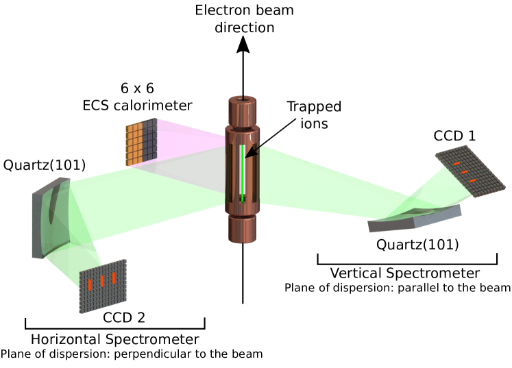
X-rays emitted by trapped ions are observed at an angle of with respect to the electron beam propagation axis. Owing to the unidirectional electron beam, the emitted X-rays are usually anisotropic and polarized. To quantify the X-ray polarization, we utilized two imaging, high-resolution, spherically bent crystal spectrometers, dubbed as the EBIT high-resolution X-ray Spectrometer (EBHiX) (Beiersdorfer et al., 2016a, b; Hell et al., 2016). These are mounted parallel and perpendicular to the electron beam propagation axis, as depicted in Fig. 1. EBHiX adopts design parameters from spherically bent crystal spectrometers used for tokamaks (Bitter et al., 2004). It is designed such that the spatial focus coincides on the detector plane with the spectral focus of the Johann geometry, i.e., , with a crystal radius of curvature and Bragg angle . The source position then follows from the focal relations of a spherical mirror. The EBHiXs are designed around a nearly fixed nominal Bragg angle of 51.3∘ and a corresponding fixed source-to-crystal distance of 2.4 m, requiring a crystal radius of curvature of 67.2 cm. We used two identical quartz (101) crystals, with a spacing of 6.687 Å and a typical intrinsic resolving power, , of 10,000 (Beiersdorfer et al., 2016b). Both crystals are affixed to a small rotatable mount, which allows fine adjustment of the central Bragg angle to make small energy-range changes. X-rays are recorded with nitrogen-cooled charge-coupled devices (CCDs) measuring pixels, with each pixel having an area of . The vacuum of each EBHiX spectrometer is separated from EBIT-I by an aluminized polyimide window (0.1 m Al / 1.0 m polyimide).
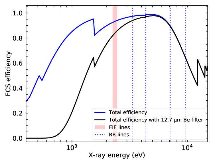
To observe X-rays from a wide energy band, we used the EBIT Calorimeter Spectrometer (ECS), a microcalorimeter array built at the NASA/Goddard Space Flight Center (Porter et al., 2004, 2008, 2009). The ECS array, operated at mK, consists of two types of pixels: (a) low-energy pixels, optimized for 0.1 to 10 keV, having m thick HgTe absorbers with an area of , giving a quantum efficiency of 95% and an excellent energy resolution of 5 eV full-width-half-maximum (FWHM) at 6 keV, and (b) high-energy pixels, covering a range from 0.5 to 100 keV, having an area of and m thick HgTe absorbers, which provide a much higher quantum efficiency, at high energies, of 32% at 60 keV. The ECS in its current configuration has four optical blocking filters in front of the array, totalling 0.15 m aluminum and 0.24 m polyimide. In addition, there is a 0.05 m polyimide filter in the beam path to separate the ECS and EBIT-I vacua; and we also used a 12.7 m Be window to filter low-energy X-rays, particularly those from bright L-shell transitions, in order to keep the total count rate low. Figure 2 shows the total ECS quantum efficiency, including total filter transmission and absorber stopping power for low-energy pixels (see details in Thorn (2008); Hell (2017)).
Using both ECS and EBHiXs, we measured the S XV excitation cross sections at four different monoenergetic electron beam energies: 2.6, 3.6, 6.4, and 8.9 keV. These energies were selected to be above the S XV K-excitation threshold, and to probe different compositions of the line formation contributions, i.e., (a) below the excitation and the Li-like inner-shell excitation thresholds (2.6 keV), (b) to include cascades from and inner-shell ionization contributions (3.7 keV), and (c) to enable a large relative H-like ion abundance in the trap (6.4 keV). The crystal spectrometers were setup at the electron beam energy of 8.9 keV. All of these beam energies are free from dielectronic recombination (DR) and resonance excitation (RE) contributions. Both the polarization and cross sections were measured at two different charge balances in the EBIT, in order to better diagnose the effects of inner-shell ionization. The medium charge-balance (MC) state (% He- and % Li-like sulfur ions) was achieved via continuous gas injection at moderately high injection pressures of Torr, providing a constant supply of low charge-state S ions in the trap. By injecting a burst of gas with the pulsed gas injector once per EBIT cycle, immediately after the trap was dumped, we obtained a high charge-balance (HC) state (% He-like ions). The trapped ions were also dumped every 920 ms for 5 ms.
3 Data Analysis
The line intensity observed by an ECSarray at due to electron-impact excitation (EIE) in an EBIT can be described as follows (Wong et al., 1995):
| (1) |
where is the effective current density, the electron charge, the number density of heliumlike ions, the solid angle subtended by the calorimeter observing photons following EIE, the combined quantum efficiency and filter transmission at EIE energies, and is the line-emission cross section at , which can be described as
| (2) |
where is the linear polarization of emitted X-rays. The negative sign should be used for an electric-dipole (E1) transitions and positive for a magnetic-dipole (M1) transitions.
Likewise, the intensity of radiative recombination (RR) X-rays observed at can be written as
| (3) |
The dependence on the effective current density and number of heliumlike ions can be eliminated if we simultaneously measure X-rays following EIE and RR (Chantrenne et al., 1992),
| (4) |
By means of Equations 2 and 4, we can determine the total electron-impact cross section, relative to that of RR, i.e.,
| (5) |
where , as the solid angle, is energy-independent, and we observe both the RR and EIE emission using the ECS low-energy array. In this experiment, we measured and , and used theoretical in order to obtain the total line-emission cross sections.
3.1 X-ray Line Polarization
According to Beiersdorfer et al. (1996), the X-ray line intensity observed using a crystal spectrometer is
| (6) |
where and are the integrated crystal reflectivities for X-rays polarized parallel and perpendicular to the plane of dispersion, and the X-ray line polarization is
| (7) |
As mentioned above, X-rays are recorded simultaneously using two crystal spectrometers, oriented in such a way that their planes of dispersion are parallel (vertical; V) and perpendicular (horizontal; H) to the electron beam propagation direction. The line intensity observed by each spectrometer can then be written as
| (8) |
and
| (9) |
The two crystals are identical, and the plane of dispersion of the vertical spectrometer is rotated by 90∘, as compared to that of its horizontal counterpart; thus we can write and , i.e., the perpendicular and parallel reflectivities of the vertical spectrometer are interchanged, compared to that of the horizontal, when assuming the same reference frame for the orientation of and . Using this relation to solve Eqs. 8 and 9 for and , and substituting them in Eq. 7, we derive an expression for the degree of linear polarization of the X-rays, as a function of the observable intensities by the two crystal spectrometers:
| (10) |
where the ratio depends on the Bragg angle , and can be estimated by for a mosaic crystal, and for a perfect crystal. Real crystals typically have values between these two limits (Beiersdorfer et al., 1996); however, we believe that the crystals used in our experiment are close to perfect. We therefore calculated the values assuming perfect crystals, using X0h111https://x-server.gmca.aps.anl.gov/x0h.html, which calculates the integrated reflectivities for quartz(101) in the energies of interest (2.4–2.5 keV) using data from Henke et al. (1993). These values were further verified using the X-ray Oriented Program (XOP; Sánchez del R´ıo & Dejus, 2011) (see details in MacDonald et al. (2021)).
The diffracted X-rays are recorded with CCD cameras, stabilized at C, ensuring low thermal noise and dark current during their operations. The CCD images were filtered for readout noise, cosmic rays, and other background events, following the method described by Pych (2004). Subsequent to these corrections, the sum of all data is projected onto the axis corresponding to the dispersion direction. Several images, each with an hour’s exposure, were obtained at each electron beam energy. The spectra from all exposures were added together in order to improve the signal-to-noise ratio.
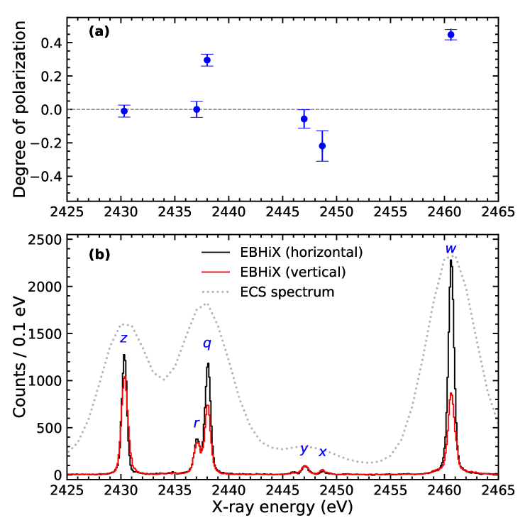
Figure 3 shows an example of a summed spectrum at 6.5 keV of beam energy, with a medium charge-balance setting. The wavelength calibrations for both spectrometers were performed using the theoretical value of line from Drake (1986), and the experimentally measured value of line of S XV (Hell et al., 2016, relative to Drake (1986)). The observed spectral peaks are then fitted using multiple Voigt functions, i.e., a convolution of Lorentz and Gaussian functions. The forbidden line at 2430 eV has a very narrow natural line width ( eV, see Crespo López-Urrutia et al. (2006)) compared to our instrumental resolution. This line allows us to determine the spectral-line broadening due to the Doppler motion of the trapped ions and due to any contribution of an intrinsic spectrometer line-spread function. Based on the axial trap depth ( V), the expected initial ion temperature (140 eV), and the crystal spectrometer line shape (MacDonald et al., 2021), the observed Gaussian width, which is 0.47-eV FWHM at 2430 eV (200 eV), should be dominated by the Doppler width, while the dominant contribution to the Lorentzian width is due to the instrument, with a negligible part due to the natural linewidth. Thus, in our fitting procedure, the Gaussian width obtained from line is shared between all peaks, while Lorentzian widths, representing the sum of instrument and natural line widths, are allowed to vary, as are the peak centroids and amplitudes.
Any photon-energy independent differences between the two crystal spectra that may arise from differences in their geometry and efficiency can be corrected using an unpolarized line for cross-normalization. X-ray lines with total angular momentum in the upper level of are unpolarized (Balashov et al., 2000). In this experiment, we used an unpolarized line, (excited state ), from lithiumlike S XIV at 2437 eV to normalize the relative efficiencies of the vertical and horizontal spectrometers.
Finally, the normalized intensities and relative reflectivities, , obtained from XOP are used in Eq. 10 to determine the degree of linear polarization of an X-ray line following the EIE. The uncertainty in the measured degree of polarization includes contributions from statistical fitting error of the line intensities, background removal, crystal reflectivities, and the relative efficiency normalization between the two crystal spectrometers inferred from the lithiumlike S XIV line . The results obtained for at a beam energy of 6.4 keV are shown in the top panel of Fig. 3. We followed a similar procedure for data sets with electron beam energies of 2.6, 3.6, and 8.9 keV. Given that lines and are well isolated, we checked the validity of our fitted line intensities by integrating counts over their respective energy ranges, obtaining degree-of-polarization results within the measurement uncertainty.
3.1.1 RR Cross Sections
| Radiative recombination into | Binding energy | Fitting Coefficients | ||||||||
|---|---|---|---|---|---|---|---|---|---|---|
| ion | State | (eV) | ||||||||
| H-like S XVI | 1 | 3494.2 | 0.394 | 9.176 | 199.311 | 412.093 | 463.886 | 213.774 | ||
| He-like S XV | 1 | 3221.9 | 0.188 | 4.415 | 95.322 | 196.599 | 220.678 | 101.434 | ||
| H-like S XVI | 2 | 874.4 | 0.042 | 0.800 | 30.393 | 60.336 | 67.080 | 31.050 | ||
| H-like S XVI | 2 | 874.5 | 0.005 | 0.182 | 2.416 | 7.469 | 12.594 | 6.614 | ||
| H-like S XVI | 2 | 871.5 | 0.010 | 0.353 | 4.564 | 15.153 | 25.245 | 13.210 | ||
| He-like S XV | 2 | 774.3 | 0.011 | 0.225 | 6.910 | 14.167 | 15.998 | 7.470 | ||
| He-like S XV | 2 | 792.8 | 0.023 | 0.410 | 20.396 | 39.218 | 43.028 | 19.821 | ||
| He-like S XV | 2 | 776.0 | 0.001 | 0.001 | 0.438 | 1.624 | 2.532 | 1.279 | ||
| He-like S XV | 2 | 775.6 | 0.003 | 0.096 | 1.295 | 4.890 | 7.606 | 3.843 | ||
| He-like S XV | 2 | 761.5 | 0.003 | 0.093 | 1.243 | 4.699 | 7.416 | 3.771 | ||
| He-like S XV | 2 | 774.0 | 0.004 | 0.153 | 2.033 | 8.331 | 12.868 | 6.501 | ||
| Li-like S XIV | 2 | 706.7 | 0.033 | 0.605 | 26.369 | 55.433 | 64.199 | 30.534 | ||
| Li-like S XIV | 2 | 678.6 | 0.005 | 0.165 | 1.954 | 5.216 | 8.670 | 4.481 | ||
| Li-like S XIV | 2 | 676.7 | 0.010 | 0.320 | 3.692 | 10.650 | 17.470 | 9.003 | ||
| Be-like S XIII | 2 | 651.8 | 0.014 | 0.252 | 12.063 | 24.985 | 28.614 | 13.500 | ||
| Be-like S XIII | 2 | 626.9 | 0.001 | 0.039 | 0.464 | 1.306 | 2.077 | 1.055 | ||
| Be-like S XIII | 2 | 626.4 | 0.004 | 0.117 | 1.376 | 3.911 | 6.203 | 3.148 | ||
| Be-like S XIII | 2 | 625.2 | 0.006 | 0.192 | 2.208 | 6.582 | 10.346 | 5.235 | ||
| Be-like S XIII | 2 | 602.3 | 0.004 | 0.118 | 1.363 | 3.710 | 6.049 | 3.101 | ||
| Be-like S XIII | 2 | 586.2 | 0.000 | 0.000 | 0.003 | 0.007 | 0.007 | 0.003 | ||
| Be-like S XIII | 2 | 560.2 | 0.000 | 0.003 | 0.474 | 0.950 | 1.038 | 0.474 | ||
| B-like S XII | 2 | 563.3 | 0.005 | 0.149 | 1.734 | 4.918 | 7.590 | 3.791 | ||
| B-like S XII | 2 | 561.7 | 0.008 | 0.277 | 3.192 | 10.342 | 15.826 | 7.943 | ||
| C-like S XI | 2 | 503.8 | 0.001 | 0.048 | 0.569 | 1.957 | 2.957 | 1.485 | ||
| C-like S XI | 2 | 503.2 | 0.003 | 0.095 | 1.091 | 3.912 | 5.836 | 2.912 | ||
| C-like S XI | 2 | 495.2 | 0.003 | 0.090 | 1.035 | 3.621 | 5.471 | 2.743 | ||
| C-like S XI | 2 | 502.3 | 0.002 | 0.069 | 0.786 | 2.812 | 4.200 | 2.097 | ||
| C-like S XI | 2 | 487.3 | 0.001 | 0.017 | 0.201 | 0.668 | 1.035 | 0.525 | ||
| N-like S X | 2 | 436.1 | 0.003 | 0.106 | 1.214 | 5.065 | 7.541 | 3.795 | ||
| N-like S X | 2 | 446.8 | 0.002 | 0.079 | 0.908 | 3.937 | 5.770 | 2.888 | ||
| N-like S X | 2 | 430.8 | 0.001 | 0.029 | 0.342 | 1.344 | 2.038 | 1.032 | ||
| N-like S X | 2 | 430.6 | 0.000 | 0.009 | 0.102 | 0.418 | 0.627 | 0.317 | ||
| N-like S X | 2 | 398.2 | 0.000 | 0.001 | 0.118 | 0.216 | 0.211 | 0.087 | ||
| O-like S IX | 2 | 378.5 | 0.003 | 0.091 | 1.027 | 4.545 | 6.651 | 3.306 | ||
| O-like S IX | 2 | 377.2 | 0.000 | 0.016 | 0.183 | 0.838 | 1.225 | 0.609 | ||
| O-like S IX | 2 | 377.5 | 0.001 | 0.050 | 0.563 | 2.546 | 3.721 | 1.851 | ||
| O-like S IX | 2 | 371.0 | 0.000 | 0.000 | 0.002 | 0.006 | 0.010 | 0.005 | ||
| F-like S VIII | 2 | 327.4 | 0.003 | 0.088 | 0.951 | 4.518 | 6.403 | 3.112 | ||
| F-like S VIII | 2 | 326.1 | 0.000 | 0.013 | 0.138 | 0.662 | 0.939 | 0.456 | ||
| Ne-like S VII | 2 | 279.2 | 0.002 | 0.048 | 0.048 | 2.527 | 3.452 | 1.628 | ||
We used the Flexible Atomic Code (FAC, Gu, 2008)222https://github.com/flexible-atomic-code/fac to calculate the radiative recombination (RR) cross sections. Similarly to Zhang (1998), FAC uses a fully relativistic distorted wave (DW) method to calculate non-resonant photoionization (PI) and RR processes. RR cross sections are obtained via detailed balance from PI cross sections. With respect to highly charged ions, electron correlation effects are less important for PI and RR processes. Thus, RR cross sections can be calculated with an accuracy of 5% or even better (Saloman et al., 1988; Scofield, 1989; Brown et al., 2006; Chen & Beiersdorfer, 2008).
We also used FAC to calculate the polarization of X-rays emitted following the RR process, as photons are observed at 90∘ relative to the direction of electron impact in our experiment. To provide an energy-dependent RR cross sections for S VI – XVI ions, we fit a fifth-order polynomial in the variable , with given in keV, to the calculated cross sections (Chen et al., 2005). The fitting parameters for the obtained RR cross sections of S XVI – VII ions in the range of 1.5–10 keV are listed in Tab. 1.
3.1.2 RR Line Intensity
The wide bandpass of the ECS microcalorimeter allows us to simultaneously measure X-rays due to RR and EIE. The energy scale of the ECS was calibrated using several measurements of - and -shell EIE lines from different hydrogenlike and heliumlike O, Ne, Si, S, Ar, Fe, Ni, Ge, Kr, and Ne-like Ba ions. Each low-energy and high-energy pixel was individually calibrated, using a fifth-order polynomial function. The spectrum is then normalized by the ECS efficiency curve including a Be filter, as discussed in Sec. 2 and shown in Fig. 2. Further details regarding the ECS efficiency and associated uncertainties can be found in Thorn (2008) and Hell (2017). Figure 4(b) shows an example of an RR spectrum measured at an electron beam energy of 2.6 keV, with medium charge-balance settings.
| Charge balance | MC (S XV1.0) | HC (S XV1.0) | |
|---|---|---|---|
| Beam energy (eV) | S XIV | S XIV | O VII |
| 2650 | 1.05 | 0.08 | 0.21 |
| 3650 | 1.04 | 0.10 | 0.38 |
| 6400 | 0.80 | 0.24 | 0.16 |
| 8900 | 1.10 | ||
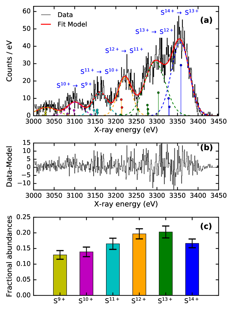
The energies of X-ray peaks from RR are given by the sum of electron beam energy and the ionization potential of the state being recombined into. We use this relation in our fitting procedure, as a first step, to obtain the precise energy of the RR lines from each charge state, as well as the effective electron beam energy, accounting for the negative space charge of the electron beam as well as ion compensation. In this step, we fix the difference between the line centroids as the ionization potential difference between different charge states, as obtained from NIST (Kramida et al., 2020). We also share the Gaussian width between all peaks, as this is dominated by a convolution of the narrow Gaussian electron beam energy distribution in the EBIT and the Gaussian instrumental resolution. Subtracting the instrument resolution in quadrature, we can thus determine the energy spread of the electron beam, e.g., eV FWHM at an electron beam energy of 2.6 keV with medium charge-balance settings. This width is enough to allow us to distinguish the RR features from different charge states of sulfur ions. However, it is very large compared to the fine-structure components of an individual RR peak (see vertical stems in Fig. 4(b) and Tab. 1). Hence, we produced synthetic RR spectra for each charge state based on the theoretical RR energies and cross sections at 90∘, and convolved them with the electron beam energy spread obtained in the previous step. The convolved synthetic spectrum for each charge state is then fitted to the data to obtain centroids and widths. These parameters, accounting for the fine structure components, are then used to fit the experimental RR spectrum to extract RR intensities.
Using Eq. 3, we inferred the relative charge balance of the trapped ions by taking the ratios of the measured RR intensities and cross sections. The derived relative ion abundances are shown in Fig. 4(a) and in Tab. 2. Note that the relative charge balance between heliumlike to lithiumlike S was also confirmed using the line ratios observed using the two crystal spectrometers.
3.1.3 EIE Line Intensity
The extraction of EIE line intensities is more complicated when more than one charge state is involved in the analysis and lines are blended. To account for these, we used a collisional-radiative model, coupled with measured values where available, to determine the line positions and intensities.
Synthetic EIE Spectrum
We used the latest version of FAC (v1.1.5) to compute the electronic structure of a given ion. The fully relativistic distorted wave method was used to calculate the EIE cross sections. For our calculations, the ground state configurations are added as and the excited state configurations as and , where represents the number of electrons in S XV – X ions. We considered principal quantum numbers up to , ogether with all their possible angular momentum states, and included full mixing between all states in our calculations.
The directional collisions between electrons and ions inside an EBIT usually lead to nonstatistical populations of magnetic sublevels of the upper state, which produce anisotropic and polarized X-rays (Beiersdorfer et al., 1996). Therefore, EIE cross sections between the magnetic sublevels of upper and lower states were computed using FAC. The X-ray polarization is then obtained from the calculated magnetic-sublevel cross sections , and intrinsic anisotropic factors, , for each line from S X – XV ions. We also accounted for depolarization due to radiative cascades, and the transverse component of electron energy due to the cyclotron motion of electrons inside the electron beam (Gu et al., 1999). Using the optical theory of electron beam propagation by Herrmann (1958), we estimated the transversal energy component to be 180 eV. The optical theory predictions are generally found to be in good agreement with the laboratory measurements (Beiersdorfer & Slater, 2001; Shah et al., 2018).
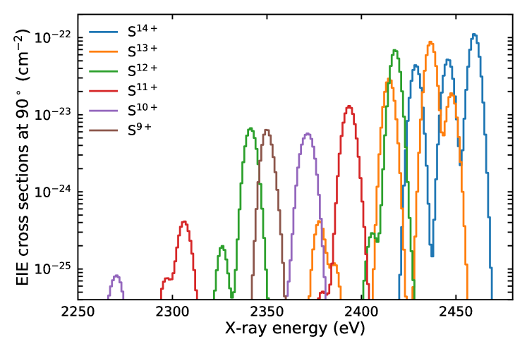
The produced atomic data, including line energies, transition rates, autoionization rates, and magnetic-sublevel-resolved EIE collision strengths, were then fed into the collisional-radiative model of FAC (Gu, 2008). This solves a system of coupled rate equations to obtain level populations for specified input experimental conditions, such as the electron beam energy and density. The resulting level populations are then used to produce a synthetic EIE spectrum at each electron beam energy. An example is shown in Fig. 5, where each line is convolved with the ECS calorimeter resolution. The synthetic spectrum allows us to account for all possible weak transitions, which have a non-negligible contribution to the measured line intensity, particularly in lower charge state Be- , B- , and C-like S ions. Furthermore, the relative intensities also take into account the inferred fractional abundances from the RR analysis.
Experimental EIE Spectrum
| Beam energy (eV) | polarization (MC) | polarization (HC) | total cross sections (MC) | total cross sections (HC) |
|---|---|---|---|---|
| 2650 | 0.56 0.03 | 0.57 0.03 | 2.65 0.18 | 2.57 0.19 |
| 3650 | 0.53 0.03 | 0.53 0.03 | 3.48 0.24 | 3.70 0.40 |
| 6400 | 0.45 0.03 | 0.50 0.02 | 3.08 0.48 | 3.45 0.26 |
| 8900 | 0.31 0.06 | 4.06 0.55 | ||
| polarization (MC) | polarization (HC) | total cross sections (MC) | total cross sections (HC) | |
| 2650 | 0.04 | 0.02 | 1.33 0.09 | 1.35 0.10 |
| 3650 | 0.04 | 0.02 | 2.01 0.14 | 1.54 0.17 |
| 6400 | 0.04 | 0.03 | 2.04 0.18 | 0.94 0.07 |
| 8900 | 0.00 0.05 | 2.60 0.36 |
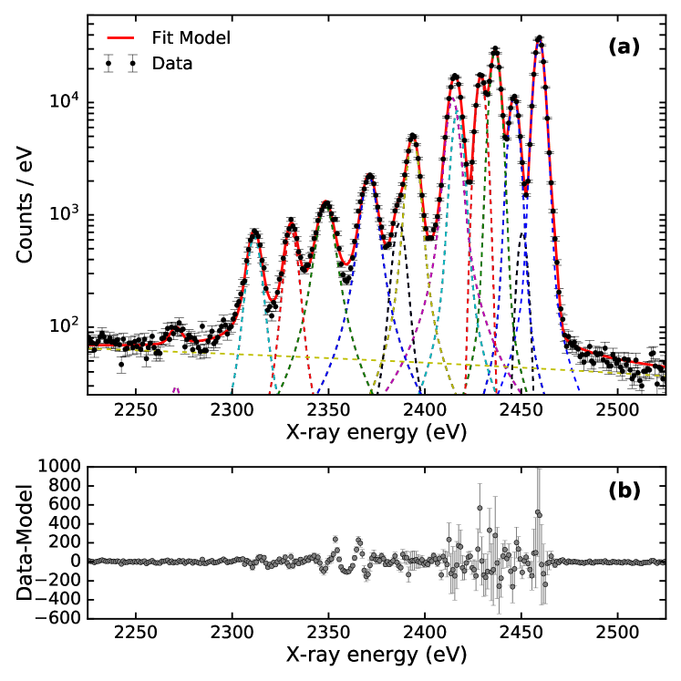
We first initialize the EIE spectrum fit using the initial values of line positions and relative intensities from the synthetic spectrum. In our fitting procedure, we use a single value of the Gaussian width for the Voigt profiles, representing the quadrature sum of the core of the calorimeter line spread function and Doppler broadening of the ions, which is tied to the forbidden line . We allowed the Lorentzian width to vary for each line; this parameter empirically accounts for the natural line widths of the lines, as well as the representation of multiple grouped satellite lines of lower charge states with similar energies, and also a small additional contribution from the calorimeter line spread function. Moreover, the line positions are allowed to vary within one FWHM to account for residual uncertainties in the transition energies, and relative intensities can vary freely to account for any differences that may stem from the polarization and cross section calculations. The background is mostly due to bremsstrahlung. We used a linear function to model it in the present energy range. Using these constraints, we obtained good fits to EIE spectra measured at each electron beam energy. An example EIE spectrum, acquired at 2.6 keV beam energy and with medium charge balance, is shown in Fig. 6 together with our best-fit model.
4 Results and Discussion
4.1 Degree of Linear Polarization
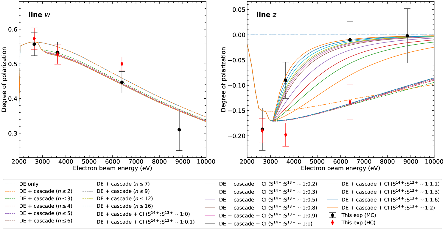
Table. 3 shows the measured degree of linear polarization of lines and at four different electron beam energies. Our measured values for lines and agree very well with the values predicted by the distorted-wave method, within uncertainty limits (Fig. 7). The resonance line, , shows a positive degree of polarization, which suggests that it is polarized parallel to the quantization axis of the electron beam propagation direction axis. This is due to the fact that the magnetic sublevel of the upper state is predominantly populated relative to that of following direct excitation from the ground state, resulting in nonzero alignment (Inal & Dubau, 1987; Surzhykov et al., 2006).
Conversely, for direct excitation of the upper state, the populations of magnetic sublevels and are identical at any given electron-impact energy. Thus, the alignment is zero, and consequently, the degree of polarization for line is zero. Our basic two-level () calculation also predicts the same for line (Fig. 7, dashed-dotted line). However, we observed a negative degree of polarization. This is because the upper level of line is mostly populated by cascades from higher-lying levels (Beiersdorfer et al., 1996; Hakel et al., 2007; Chen et al., 2015). At 2.6 keV beam energy, only cascades from levels are possible, and they contribute significantly to the degree of polarization of line . Above this beam energy, the high states are open for direct excitation from the ground state. Therefore, at 3.6, 6.4, and 8.9 keV beam energies, strong cascades from further decrease the degree of polarization for both lines and . The dashed curves in Fig. 7 show changes in X-ray polarization due to cascades from different levels, up .
For beam energies above 3.14 keV, collisional inner-shell ionization of lithiumlike S XIV ions plays an important role, as it populates the level through ionization of the lithiumlike ground state, (Inal & Dubau, 1987). We used FAC to calculate the magnetic sublevel populations following collisional ionization, in order to check its effect on the polarization. We vary the fractional abundance of S XIV ions relative to that of S XV ions in these calculations. The solid curves in Fig. 7 show polarization predictions, including both cascades and CI, with a varying relative ion population. The contribution to line line from CI is essentially unpolarized, as both magnetic sublevels, , of lithiumlike ground state have identical values in an axially symmetric system (Mehlhorn, 1968). Therefore, the larger the fraction of the upper state of the line populated via CI of S XIV, the greater the reduction in the observed degree of polarization. This effect becomes more significant with increasing electron beam energy, as the relative importance of CI increases with increasing collision energy. In fact, our experiment with medium charge-balance settings shows excellent agreement with the theory when CI is accounted for using the charge balance measured from the strengths of the RR peak strengths and the inner-shell satellite lines and . Conversely, the predicted polarization for the high charge-balance measurements has only a small correction from inner-shell ionization, and a model only including cascades agrees very well with our measurements, as the fractions of S XIV ions are relatively small compared to those of S XV.
The Breit interaction (Breit, 1929), a relativistic correction to the instantaneous Coulomb repulsion, is usually important for high- ions (Fritzsche et al., 2009), but it may considerably alter the degree of polarization for low- and medium- ions (Shah et al., 2015). Moreover, such relativistic effects become progressively more significant as the incident electron-impact energy increases (Reed & Chen, 1993). We considered these effects in our calculations, but we did not find a substantial change in the degree of linear polarization for lines and . Moreover, two-photon radiative decay can also affect the line polarizations (Derevianko & Johnson, 1997; Surzhykov et al., 2010; Dipti et al., 2020). Our level-population calculations automatically take this into account, based on two-photon rates calculated by Drake (1986). The external magnetic and electric fields present in the trapping region of an EBIT could also modify the magnetic-sublevel population, thus the degree of polarization. However, in our experiment, the direction of the external magnetic field is the same as that of the electron beam, so the magnetic-sublevel populations should not be redistributed.
4.2 Total EIE Cross Sections
The EIE cross sections at an observed angle of 90∘ are obtained by normalizing the EIE intensities with RR cross sections and RR intensity. Finally, the 90∘ cross sections are corrected for measured polarization to extract the total line-emission cross sections. The uncertainties in the derived cross sections include contributions from all possible terms, including statistical fitting uncertainties on the RR (%), and EIE intensities (%), detector efficiency, and filter transmissions (%), theoretical differential RR cross sections (%), and, as explained in Sec. 3.1, the uncertainty associated with the measured degree of polarization (5-7%). The overall uncertainty in the measured cross sections is on the order of %.
In addition, we also checked background ions with ionization energies near to that of S XV ions, such as O VIII and N VII ions, which may contribute to the observed RR spectrum. In such a case, the S XV RR =2 line can blend with RR =1 lines from O VIII and N VII at any given electron beam energy. We cannot directly resolve these background lines in the RR spectrum, as the electron beam energy spread is much larger than the difference between the ionization potentials of background ions. If present, however, the fractional abundances of such ions can be estimated based on the observed and expected strengths of collisionally-excited hydrogenlike Lyman- line. In order to estimate line strengths of contaminant ions, we have removed the Be filter from the beam path. In the case of the MC experiment, we observed only a minor enhancement over a continuum at eV N VII Ly and eV O VIII Ly energies. Having taken into account the ECS efficiency (Fig. 2), we find that the data indicates a negligible contribution to the RR spectrum. On the other hand, we see a strong oxygen line at 653 eV for the high charge-balance experiment. This may be due to the fact that we used a pulsed injection for HC, in contrast to a continuous injection of S for the MC experiment. In the latter case, the oxygen ion buildup in the trap may have been inhibited by the continuous flow of sulfur into the trap.
For HC data, the fractional abundance ratio between O VIII and S XV can be estimated using Eq. 1, i.e., by taking the ratio between and . However, here we must also consider attenuation from molecular contaminants that may freeze on the filters. The main expected contaminants primarily contain hydrogen, oxygen, and nitrogen. As the photoelectric absorption cross section above threshold scales approximately as , any such contaminant would produce the same transmission curve at energies above the oxygen -edge, assuming a given optical depth at a given photon energy. We therefore treat the contaminant as a layer of oxygen atoms. We measured the optical depth decrement between two energies by taking the intensity ratio of the O Ly and Ly lines, and comparing them to previously measured ratios using the same EBIT. The O Ly/Ly intensity ratio at high impact energies becomes constant (see Fig. 23 of Beiersdorfer (2003)). Thus, we took the weighted average of measured ratios in the range of 2–10 keV beam energies (6.13 0.11). Based on the optical depth decrement inferred from the measured ratio, we estimated the areal density of oxygen contaminants to be g cm-2; the equivalent layer thickness was m, assuming a fiducial density of 1 g cm-3. We corrected the total filter transmission for the contaminant, and obtained the relative fractional abundance between O and S ions. We found these to be %, %, and % for 2.6, 3.6, and 6.4 keV, respectively, for HC measurements. These oxygen fractions are used then to obtain the real RR intensity due to S XV ions only. An extra RR line, based on the ionization potential of O VIII, is added, and its flux is constrained to the inferred ratios in the fitting procedure, as explained in Sec. 3.1.2. The inferred S XV RR intensity and associated uncertainty from this step are then used to obtain the total cross sections for HC measurements.
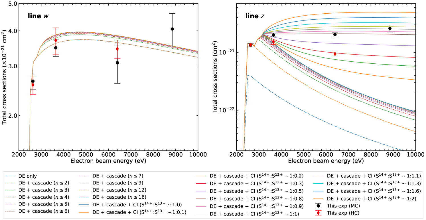
The final cross section results are listed in Tab. 3 and shown in Fig. 8. Distorted wave predictions using FAC show excellent agreement with the measured cross sections, given that we account for necessary contributions from cascades and collisional inner-shell ionization, as also explained in Sec. 4.1.
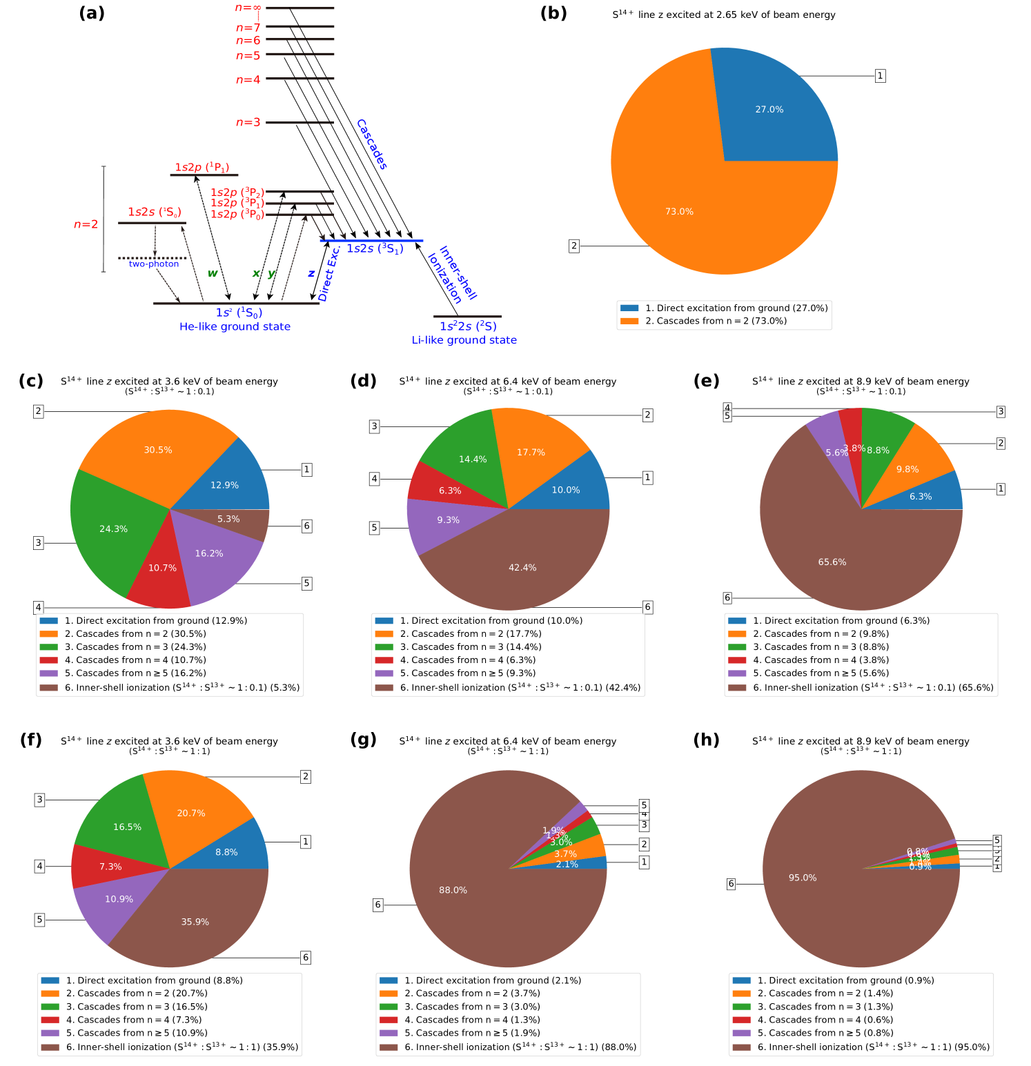
The measured cross sections for the resonance line, , show very good agreement with the theory. Cascades within , and from high- levels, modify the cross sections by only a very small amount (6%–7%). In contrast, the cross sections for line are significantly altered by radiative cascades. For example, cascades from within increase the cross section of by % at 2.7 keV beam energy, as compared to direct excitation from the ground (Fig. 9, panel (b)). As the electron-impact energy increases, cascades from high states further enhance the emission cross sections of line . Figure 8 shows cascade contributions from different levels, up , as dashed lines.
In addition, as explained earlier, collisional inner-shell ionization of lithiumlike S XIV ions starts to contribute to line above 3.14 keV beam energy. As shown in Fig. 9, panels (c) and (f), CI contributes as much as % to the measured cross sections at a 3.6 keV beam energy, depending on the relative abundances of S XIV and S XV. This contribution increases significantly at high electron-impact energies, and dominates over the usual contributions from cascades and direct excitations. For example, our experiment shows that CI enhances the cross sections of line by % at 6.4 keV beam energy, when the Li-like S ion concentration is increased from 24% to 80% in the trap. This agrees very well with distorted wave predictions of 53.4% enhancement. As depicted in Fig. 9, panels (d), (e), (g), and (h), CI completely dominates the cross sections at high beam energies of 6.4 and 8.9 keV, even if the S XIV fraction is very low compared to that of S XV. It is therefore imperative to take CI into account for the spectral modeling of high-temperature plasmas, not only those in equilibrium conditions, but particularly those that are out of equilibrium.
Our systematic measurements under two different charge-balance conditions clearly distinguish between predictions with different fractions of S XIV relative to that of S XV and show that both cascades and CI are essential for accurate predictions of emission cross sections for line . Furthermore, experimental agreement between data taken at a 2.6 keV beam energy with two different charge balances indicates that the overall analysis, the extracted charge balance, as well as the theoretical treatment of cascades and CI, are reliable.
Line may also be populated via charge exchange (CX) and RR into H-like S XVI at higher electron beam energies, and this may modify the inferred polarization and cross sections. The cross sections for RR into levels are on the order of cm2 (see Tab. 1), which are at least 3-4 orders of magnitude smaller compared to line-formation cross sections due to direct excitation, cascades, and inner-shell ionization processes. On the other hand, the CX cross section are on the order of cm2, where is the ionic charge (Phaneuf, 1983; Janev & Winter, 1985; Otranto et al., 2006). The CX rate can be represented as the product of , where and are the ion and neutral densities, and is the collision velocity of ions and neutrals inside an EBIT, which is set by the ion temperature. Previously, we measured CX between S XVI – XVII and SF6 using the same EBIT and ECS detector (Betancourt-Martinez et al., 2014). By comparing the count rate, populations of bare, hydrogenic, and heliumlike S ions, and gas injection pressure used in that experiment, as in this one, we estimated that the CX rate contributing to line is approximately three orders of magnitude smaller than the electron-impact excitation rate for our MC measurements. Furthermore, our HC measurements used a pulsed gas injector to introduce neutrals to the trap only at the beginning of the charge-breeding cycle. Given the very low background pressure ( Torr) at the center of the trap, and the lack of injection after the breeding part of the HC measurement cycle, X-rays from CX must be negligible. Data taken at 2.6 and 3.6 keV beam energies must be even less affected, due to lower production of H-like S ions, resulting in fewer targets for CX that can produce S K-shell emission lines. Thus, population of the level through RR and CX processes, is negligible for the present experiment. Furthermore, dielectronic recombination and resonance excitation are not relevant for the present experimental electron beam energies used here, and 3-body recombination contribution should be negligible, due to the low density of the EBIT plasma (Levine et al., 1988).
5 Summary and Conclusions
We have measured the degree of linear polarization and total effective line-emission cross sections for the crucial heliumlike resonance and forbidden lines of S XV, using the combination of the LLNL EBIT-I facility with two high-resolution EBHiX crystal spectrometers, together with the broad-band ECS microcalorimeter. Our technique enabled us to measure the emission cross sections to better than 10%, and allowed us to disentangle the relative contributions from cascades and from inner-shell ionization of Li-like S XIV to the key forbidden line, . Our systematic experiment also benchmarks FAC distorted-wave predictions for both the X-ray line polarization and total line-emission cross sections, and demonstrates that cascades and inner-shell ionization contributions should be accounted for in predictions of heliumlike line-emission cross sections.
In astrophysical conditions where the ionization balance is not solely determined by the mean electron temperature of the plasma, collisional inner-shell ionization processes can contribute a considerable fraction of the line emission, as shown in this work. Therefore, our data may also help with the identification of nonequilibrium conditions that may exist in transient X-ray sources, such as young supernova remnants, accretions shocks, and solar flares (Watanabe et al., 1995; Rasmussen et al., 2001; Porquet et al., 2010; Decaux et al., 1997; Katsuda et al., 2012; Suzuki et al., 2020). Such diagnostics, however, are heavily dependent on the underlying atomic data compiled in spectral modeling codes, such as SPEX (Kaastra et al., 1996) and AtomDB (Foster et al., 2012) spectral modeling codes. For example, the compiled collision strengths for the forbidden line in Fe XXV in these codes critically differ by more than 40% (Hitomi Collaboration et al., 2018a). Therefore, our experimental data could also be used to stringently test the accuracy of these codes. This is indeed a crucial task in view of the next generation of X-ray satellites, namely XRISM (Tashiro et al., 2018) and Athena (Barret et al., 2016), which will reach exceptional spectral-energy resolutions and higher sensitivities, as shown by Hitomi (Hitomi Collaboration et al., 2016, 2017).
References
- Ali et al. (2011) Ali, S., Mahmood, S., Orban, I., et al. 2011, J. Phys. B: At. Mol. Opt. Phys., 44, 44
- Audard et al. (2001) Audard, M., Behar, E., Güdel, M., et al. 2001, A&A, 365, L329
- Balashov et al. (2000) Balashov, V. V., Grum-Grzhimailo, A. N., & Kabachnik, N. M. 2000, Polarization and Correlation Phenomena in Atomic Collision (Kluwer Academics/ Plenum Publishers)
- Barret et al. (2016) Barret, D., Lam Trong, T., den Herder, J.-W., et al. 2016, in Society of Photo-Optical Instrumentation Engineers (SPIE) Conference Series, Vol. 9905, Proc. SPIE, 99052F
- Beiersdorfer (2003) Beiersdorfer, P. 2003, ARA&A, 41, 41
- Beiersdorfer et al. (2009) Beiersdorfer, P., Brown, G. V., Clementson, J. H. T., et al. 2009, J. Phys. Conf. Ser., 163, 163
- Beiersdorfer et al. (2016a) Beiersdorfer, P., Magee, E. W., Brown, G. V., et al. 2016a, Rev. Sci. Instrum., 87, 063501
- Beiersdorfer et al. (2016b) Beiersdorfer, P., Magee, E. W., Hell, N., & Brown, G. V. 2016b, Rev. Sci. Instrum., 87, 11E339
- Beiersdorfer et al. (1990) Beiersdorfer, P., Osterheld, A. L., Chen, M. H., et al. 1990, Phys. Rev. Lett., 65, 65
- Beiersdorfer et al. (1992) Beiersdorfer, P., Phillips, T. W., Wong, K. L., Marrs, R. E., & Vogel, D. A. 1992, Phys. Rev. A, 46, 46
- Beiersdorfer & Slater (2001) Beiersdorfer, P. & Slater, M. 2001, Phys. Rev. E, 64, 64
- Beiersdorfer et al. (1996) Beiersdorfer, P., Vogel, D. A., Reed, K. J., et al. 1996, Phys. Rev. A, 53, 53
- Betancourt-Martinez et al. (2014) Betancourt-Martinez, G. L., Beiersdorfer, P., Brown, G. V., et al. 2014, Phys. Rev. A, 90, 90
- Bianchi et al. (2005) Bianchi, S., Matt, G., Nicastro, F., Porquet, D., & Dubau, J. 2005, MNRAS, 357, 599
- Biedermann et al. (2002) Biedermann, C., Radtke, R., & Fournier, K. B. 2002, Phys. Rev. E, 66, 66
- Bitter et al. (2008) Bitter, M., Hill, K. W., Goeler, S. V., et al. 2008, Can. J. Phys., 86, 291
- Bitter et al. (2004) Bitter, M., Hill, K. W., Stratton, B., et al. 2004, Rev. Sci. Instrum., 75, 3660
- Blumenthal et al. (1972) Blumenthal, G. R., Drake, G. W. F., & Tucker, W. H. 1972, ApJ, 172, 205
- Breit (1929) Breit, G. 1929, Phys. Rev., 34, 34
- Brown et al. (2006) Brown, G. V., Beiersdorfer, P., Chen, H., et al. 2006, Phys. Rev. Lett., 96, 253201
- Chantrenne et al. (1992) Chantrenne, S., Beiersdorfer, P., Cauble, R., & Schneider, M. B. 1992, Phys. Rev. Lett., 69, 69
- Chen & Beiersdorfer (2008) Chen, H. & Beiersdorfer, P. 2008, Can. J. Phys., 86, 86
- Chen et al. (2005) Chen, H., Beiersdorfer, P., Scofield, J. H., et al. 2005, ApJ, 618, 618
- Chen et al. (2002) Chen, H., Beiersdorfer, P., Scofield, J. H., et al. 2002, ApJ, 567, 567
- Chen et al. (2006) Chen, H., Gu, M. F., Beiersdorfer, P., et al. 2006, ApJ, 646, 646
- Chen et al. (2015) Chen, Z.-B., Dong, C.-Z., & Jiang, J. 2015, Phys. Scr., 90, 90
- Crespo López-Urrutia et al. (2006) Crespo López-Urrutia, J. R., Beiersdorfer, P., & Widmann, K. 2006, Phys. Rev. A, 74, 012507
- Decaux et al. (1997) Decaux, V., Beiersdorfer, P., Kahn, S. M., & Jacobs, V. L. 1997, ApJ, 482, 482
- Decaux et al. (1995) Decaux, V., Beiersdorfer, P., Osterheld, A., Chen, M., & Kahn, S. M. 1995, ApJ, 443, 464
- Del Zanna, G. et al. (2015) Del Zanna, G., Dere, K. P., Young, P. R., Landi, E., & Mason, H. E. 2015, A&A, 582, 582
- Derevianko & Johnson (1997) Derevianko, A. & Johnson, W. R. 1997, Phys. Rev. A, 56, 1288
- Dipti et al. (2020) Dipti, Buechele, S. W., Gall, A. C., et al. 2020, J. Phys. B: At., Mol. Opt. Phys., 53, 53
- Doschek et al. (1971) Doschek, G. A., Meekins, J. F., Kreplin, R. W., Chubb, T. A., & Friedman, H. 1971, ApJ, 170, 170
- Dovčiak et al. (2004) Dovčiak, M., Karas, V., & Matt, G. 2004, MNRAS, 355, 355
- Drake (1986) Drake, G. W. F. 1986, Phys. Rev. A, 34, 34
- Foster et al. (2012) Foster, A. R., Ji, L., Smith, R. K., & Brickhouse, N. S. 2012, ApJ, 756, 128
- Freeman et al. (1971) Freeman, F. F., Gabriel, A. H., Jones, B. B., & Jordan, C. 1971, Philosophical Transactions of the Royal Society of London Series A, 270, 127
- Fritzsche et al. (2009) Fritzsche, S., Surzhykov, A., & Stöhlker, T. 2009, Phys. Rev. Lett., 103, 103
- Gabriel (1972) Gabriel, A. H. 1972, MNRAS, 160, 99
- Gabriel & Jordan (1969) Gabriel, A. H. & Jordan, C. 1969, MNRAS, 145, 241
- Gall et al. (2020) Gall, A. C., Dipti, Buechele, S. W., et al. 2020, J. Phys. B: At. Mol. Opt. Phys., 53, 53
- Gu (2008) Gu, M. F. 2008, Can. J. Phys, 86, 675
- Gu et al. (1999) Gu, M. F., Kahn, S. M., Savin, D. W., et al. 1999, ApJ, 518, 518
- Hakel et al. (2007) Hakel, P., Mancini, R. C., Harris, C., et al. 2007, Phys. Rev. A, 76, 76
- Harra-Murnion et al. (1996) Harra-Murnion, L. K., Phillips, K. J. H., Lemen, J. R., et al. 1996, A&A, 308, 670
- Haug (1972) Haug, E. 1972, Solar Phys., 25, 25
- Haug (1981) Haug, E. 1981, Solar Phys., 71, 71
- Hell (2017) Hell, N. 2017, Benchmarking transition energies and emission strengths for X-ray astrophysics with measurements at the Livermore EBITs, PhD thesis, Dr. Karl Remeis-Sternwarte & ECAP, Universität Erlangen-Nürnberg, Sternwartstr. 7, 96049 Bamberg, Germany; Lawrence Livermore National Laboratory, 7000 East Ave, Livermore CA 94550, USA
- Hell et al. (2016) Hell, N., Brown, G. V., Wilms, J., et al. 2016, ApJ, 830, 830
- Henderson et al. (1990) Henderson, J. R., , Beiersdorfer, P., et al. 1990, Phys. Rev. Lett., 65, 65
- Henke et al. (1993) Henke, B. L., Gullikson, E. M., & Davis, J. C. 1993, At. Data Nucl. Data Tables, 54, 181
- Herrmann (1958) Herrmann, G. 1958, J. Appl. Phys., 29, 29
- Hitomi Collaboration et al. (2016) Hitomi Collaboration et al. 2016, Nature, 535, 117
- Hitomi Collaboration et al. (2017) Hitomi Collaboration et al. 2017, Nature, 551, 478
- Hitomi Collaboration et al. (2018a) Hitomi Collaboration et al. 2018a, PASJ, 70, 12
- Hitomi Collaboration et al. (2018b) Hitomi Collaboration et al. 2018b, PASJ, 70, 10
- Hu et al. (2012) Hu, Z., Han, X., Li, Y., et al. 2012, Phys. Rev. Lett., 108, 108
- Inal & Dubau (1987) Inal, M. K. & Dubau, J. 1987, J. Phys. B: At. Mol. Opt. Phys., 20, 20
- Janev & Winter (1985) Janev, R. & Winter, H. 1985, Phys. Rep., 117, 117
- Kaastra et al. (2001) Kaastra, J. S., Ferrigno, C., Tamura, T., et al. 2001, A&A, 365, L99
- Kaastra et al. (1996) Kaastra, J. S., Mewe, R., & Nieuwenhuijzen, H. 1996, in 11th Colloq. on UV and X-ray Spectroscopy of Astrophysical and Laboratory Plasmas, ed. K. Yamashita & T. Watanabe (Tokyo: Universal Academy Press), 411–414
- Kahn et al. (2001) Kahn, S. M., Leutenegger, M. A., Cottam, J., et al. 2001, A&A, 365, L312
- Kallman (2004) Kallman, T. 2004, Adv. Space Res., 34, 34
- Katsuda et al. (2012) Katsuda, S., Tsunemi, H., Mori, K., et al. 2012, ApJ, 756, 49
- Kramida et al. (2020) Kramida, A., Yu. Ralchenko, Reader, J., & and NIST ASD Team. 2020, NIST Atomic Spectra Database (ver. 5.8), [Online]. Available: http://physics.nist.gov/asd. National Institute of Standards and Technology, Gaithersburg, MD.
- Krawczynski et al. (2011) Krawczynski, H., III, A. G., Guo, Q., et al. 2011, Astropart. Phys., 34, 34
- Laming (1990a) Laming, J. M. 1990a, ApJ, 357, 275
- Laming (1990b) Laming, J. M. 1990b, ApJ, 362, 219
- Leutenegger et al. (2006) Leutenegger, M. A., Paerels, F. B. S., Kahn, S. M., & Cohen, D. H. 2006, ApJ, 650, 1096
- Levine et al. (1989) Levine, M. A., Marrs, R. E., Bardsley, J. N., et al. 1989, Nucl. Instrum. Methods Phys. Res., Sect. B, 43, 431
- Levine et al. (1988) Levine, M. A., Marrs, R. E., Henderson, J. R., Knapp, D. A., & Schneider, M. B. 1988, Phys. Scr., 22, 157
- Lindroth et al. (2020) Lindroth, E., Orban, I., Trotsenko, S., & Schuch, R. 2020, Phys. Rev. A, 101, 101
- MacDonald et al. (2021) MacDonald, M. J., Widmann, K., Beiersdorfer, P., et al. 2021, Rev. Sci. Instrum., 92, 92
- Mahmood et al. (2012) Mahmood, S., Ali, S., Orban, I., et al. 2012, ApJ, 754, 754
- Marrs et al. (1995) Marrs, R. E., Beiersdorfer, P., Elliott, S. R., Knapp, D. A., & Stoehlker, T. 1995, Phys. Scr., 59, 183
- Mehlhorn (1968) Mehlhorn, W. 1968, Phys. Lett. A, 26, 26
- Mewe & Schrijver (1978) Mewe, R. & Schrijver, J. 1978, A&A, 65, 115
- Mewe & Schrijver (1980) Mewe, R. & Schrijver, J. 1980, A&A, 87, 261
- Nakamura et al. (2008) Nakamura, N., Kavanagh, A. P., Watanabe, H., et al. 2008, Phys. Rev. Lett., 100, 100
- Nayakshin (2007) Nayakshin, S. 2007, MNRAS, 376, 376
- Ness et al. (2003) Ness, J. U., Schmitt, J. H. M. M., Audard, M., Güdel, M., & Mewe, R. 2003, A&A, 407, 347
- Oppenheimer (1927) Oppenheimer, J. R. 1927, Proc. Natl. Acad. Sci. U.S.A, 13, 13
- Otranto et al. (2006) Otranto, S., Olson, R. E., & Beiersdorfer, P. 2006, Phys. Rev. A, 73, 73
- Penetrante et al. (1991) Penetrante, B. M., Bardsley, J. N., DeWitt, D., Clark, M., & Schneider, D. 1991, Phys. Rev. A, 43, 43
- Percival & Seaton (1958) Percival, I. C. & Seaton, M. J. 1958, Philos. Trans. R. Soc. A, 251, 251
- Peterson et al. (2001) Peterson, J. R., Paerels, F. B. S., Kaastra, J. S., et al. 2001, A&A, 365, L104
- Phaneuf (1983) Phaneuf, R. A. 1983, Phys. Rev. A, 28, 28
- Porquet & Dubau (2000) Porquet, D. & Dubau, J. 2000, A&AS, 143, 495
- Porquet et al. (2010) Porquet, D., Dubau, J., & Grosso, N. 2010, Space Sci. Rev., 157, 103
- Porter et al. (2008) Porter, F. S., Beiersdorfer, P., Brown, G. V., et al. 2008, J. Low Temp. Phys, 151, 1061
- Porter et al. (2009) Porter, F. S., Beiersdorfer, P., Brown, G. V., et al. 2009, in Journal of Physics Conference Series, Vol. 163, J. Phys. Conf. Ser, 012105
- Porter et al. (2004) Porter, F. S., Brown, G. V., Boyce, K. R., et al. 2004, Rev. Sci. Instrum., 75, 3772
- Pych (2004) Pych, W. 2004, Publ. Astron. Soc. Pac., 116, 116
- Rasmussen et al. (2001) Rasmussen, A. P., Behar, E., Kahn, S. M., den Herder, J. W., & van der Heyden, K. 2001, A&A, 365, L231
- Reed & Chen (1993) Reed, K. J. & Chen, M. H. 1993, Phys. Rev. A, 48, 48
- Robbins et al. (2004) Robbins, D. L., Faenov, A. Y., Pikuz, T. A., et al. 2004, Phys. Rev. A, 70, 70
- Saloman et al. (1988) Saloman, E., Hubbell, J., & Scofield, J. 1988, At. Data Nucl. Data Tables, 38, 38
- Sánchez del R´ıo & Dejus (2011) Sánchez del Río, M. & Dejus, R. J. 2011, in Proc. SPIE, Vol. 8141, Proc. SPIE, 814115
- Scofield (1989) Scofield, J. H. 1989, Phys. Rev. A, 40, 40
- Shah et al. (2016) Shah, C., Amaro, P., Steinbrügge, R., et al. 2016, Phys. Rev. E, 93, 061201
- Shah et al. (2018) Shah, C., Amaro, P., Steinbrügge, R., et al. 2018, ApJS, 234, 27
- Shah et al. (2019) Shah, C., Crespo López-Urrutia, J. R., Gu, M. F., et al. 2019, ApJ, 881, 100
- Shah et al. (2015) Shah, C., Jörg, H., Bernitt, S., et al. 2015, Phys. Rev. A, 92, 042702
- Soffitta et al. (2013) Soffitta, P., Barcons, X., Bellazzini, R., et al. 2013, Exp. Astron., 36, 36
- Sterling et al. (1997) Sterling, A. C., Hudson, H. S., & Watanabe, T. 1997, ApJ, 479, 479
- Surzhykov et al. (2006) Surzhykov, A., Jentschura, U. D., Stöhlker, T., & Fritzsche, S. 2006, Phys. Rev. A, 73, 73
- Surzhykov et al. (2010) Surzhykov, A., Volotka, A., Fratini, F., et al. 2010, Phys. Rev. A, 81, 042510
- Suzuki et al. (2020) Suzuki, H., Yamaguchi, H., Ishida, M., et al. 2020, ApJ, 900, 900
- Takács et al. (1996) Takács, E., Meyer, E. S., Gillaspy, J. D., et al. 1996, Phys. Rev. A, 54, 54
- Tamura et al. (2001) Tamura, T., Bleeker, J. A. M., Kaastra, J. S., Ferrigno, C., & Molendi, S. 2001, A&A, 379, 107
- Tashiro et al. (2018) Tashiro, M., Maejima, H., Toda, K., et al. 2018, Proc. SPIE, 10699, 10699
- Thorn (2008) Thorn, D. B. 2008, Spectroscopic Investigations of Highly Charged Ions using X-Ray Calorimeter Spectrometers, PhD thesis, University of California, Davis
- Wargelin et al. (2008) Wargelin, B. J., Beiersdorfer, P., & Brown, G. V. 2008, Can. J. Phys., 86, 151
- Watanabe et al. (1995) Watanabe, T., Haka, H., Shimizu, T., et al. 1995, Sol. Phys., 157, 169
- Weber et al. (2015) Weber, S., Beilmann, C., Shah, C., & Tashenov, S. 2015, Rev. Sci. Instrum., 86, 093110
- Weisskopf et al. (2006) Weisskopf, M. C., Elsner, R. F., Hanna, D., et al. 2006, ArXiv Astrophysics e-prints
- Wong et al. (1995) Wong, K. L., Beiersdorfer, P., Reed, K. J., & Vogel, D. A. 1995, Phys. Rev. A, 51, 51
- Zhang (1998) Zhang, H. L. 1998, Phys. Rev. A, 57, 57