High-Resolution Mid-Infrared Spectroscopy of GV Tau N: Surface Accretion and Detection of NH3 in a Young Protoplanetary Disk
Abstract
Physical processes that redistribute or remove angular momentum from protoplanetary disks can drive mass accretion onto the star and affect the outcome of planet formation. Despite ubiquitous evidence that protoplanetary disks are engaged in accretion, the process(es) responsible remain unclear. Here we present evidence for redshifted molecular absorption in the spectrum of a Class I source that indicates rapid inflow at the disk surface. High resolution mid-infrared spectroscopy of GV Tau N reveals a rich absorption spectrum of individual lines of , HCN, , and . From the properties of the molecular absorption, we can infer that it carries a significant accretion rate comparable to the stellar accretion rates of active T Tauri stars. Thus we may be observing disk accretion in action. The results may provide observational evidence for supersonic “surface accretion flows,” which have been found in MHD simulations of magnetized disks. The observed spectra also represent the first detection of in the planet formation region of a protoplanetary disk. With only comparable in abundance to HCN, it cannot be a major missing reservoir of nitrogen. If, as expected, the dominant nitrogen reservoir in inner disks is instead N2, its high volatility would make it difficult to incorporate into forming planets, which may help to explain the low nitrogen content of the bulk Earth.
1 Introduction
Stars form surrounded by disks, the repositories of excess angular momentum inherited from the molecular cloud that cannot be contained within the star alone. Physical processes that redistribute or remove disk angular momentum can drive mass accretion onto the star and affect the outcome of planet formation; e.g., giant planets that form in the disk may be swept inward along with the accretion flow. Although it is as yet unclear what physical mechanism(s) generate accretion flows, the process(es) must be robust: T Tauri stars (i.e., young stars surrounded by disks) commonly show excess UV emission produced by mass flows that reach the stellar surface (Hartmann et al. 2016).
One clue to the nature of disk accretion comes from the sizes of gaseous disks. Whereas disks in the embedded “Class I” phase of pre-main-sequence evolution are modest in size (typically au in radius), gas disks in the more evolved “Class II” phase, when infall from the molecular cloud has ceased, span a range of sizes including many much larger than 300 au (Najita & Bergin 2018; Ansdell et al. 2018). The existence of such large disks is remarkable given the multiple processes that can act to reduce disk sizes (e.g., FUV photoevaporation, companion formation, disk winds). Their existence suggests that internal angular momentum redistribution plays a large enough role in driving accretion that a significant fraction of disks grow substantially in size from the Class I to Class II phases (Najita & Bergin 2018). However there have been few observational clues to date as to the nature of the process that redistributes the angular momentum. Disk spectral line diagnostics offer the opportunity to probe the dynamics of disks for potential new insights.
Spectral features in the mid-infrared (MIR) offer the opportunity to study the dynamics and chemistry of planet formation environments. Class II (T Tauri) disks commonly reveal a MIR spectrum that is rich in emission from water and organic molecules (, HCN, ; Carr & Najita 2008, 2011; Salyk et al. 2011). The emitting areas, line profiles, and thermal-chemical properties of the emitting gas are consistent with emission from an irradiated disk atmosphere within a few au of the star, i.e., the terrestrial planet region of the disk (e.g., Najita & Ádámkovics 2017; Najita et al. 2018). In contrast to the frequent detection of MIR molecular emission, MIR molecular absorption is detected only rarely from young stars at low spectral resolution. Observations with the Spitzer Space Telescope detected molecular absorption features of HCN, , and from IRS 46 (Lahuis et al. 2006) and GV Tau (e.g., Bast et al. 2013), and from DG Tau B (Kruger et al. 2011; Pontoppidan et al. 2008). The similar molecular species and gas temperatures detected in emission and absorption suggested that the absorption features also arise in a disk atmosphere but viewed close to edge on (Bast et al. 2013; Doppmann et al. 2008).
Here we report high resolution MIR spectroscopy of the Class I source GV Tau N, which reveals a rich molecular absorption spectrum of individual lines of and HCN, as well as and the first detection of in the planet formation region of a protoplanetary disk. The resolved line profiles, which have a significant redshifted component, may provide observational evidence for a new accretion mechanism: supersonic “surface accretion flows,” which have been found in MHD simulations of magnetized disks (Zhu & Stone 2018; see also Stone & Norman 1994; Beckwith et al. 2009; Guilet & Ogilvie 2012, 2013).
A young stellar binary in the Taurus molecular cloud (d=140 pc), GV Tau (a.k.a. Haro 6–10, IRAS 04263+2426) comprises a bright optical source, GV Tau S, and an infrared companion located 1.2′′ away, GV Tau N, which dominates the MIR flux of the system (e.g., Leinert & Haas 1989; Sheehan & Eisner 2014). While GV Tau has the strongly rising 2–25 continuum characteristic of Class I sources (e.g., Furlan et al. 2008), its relatively weak gas and dust emission compared to other low-mass embedded YSOs suggests that the system lacks a significant envelope (Hogerheijde et al. 1998). That property and the poorly defined molecular outflow structure of the system (Hogerheijde et al. 1998) suggest that it is a more evolved Class I source. Spatially resolved millimeter imaging further suggests modest solid disk masses for both GV Tau N and S (Sheehan & Eisner 2014) and small dust disk sizes ( au; Guilloteau et al. 2011).
In addition to the molecular absorption bands of HCN, , and detected with Spitzer (Bast et al. 2013), the spectrum of GV Tau N also shows individual near-infrared (NIR) absorption lines of HCN, , CH4, and CO (Gibb et al. 2007; Doppmann et al. 2008; Gibb & Horne 2013; Davis et al. 2015). While CO absorption has been detected toward both Class I and Class II sources at high spectral resolution (Brittain et al. 2005; Rettig et al. 2006; Horne et al. 2012; Kruger et al. 2011; Smith et al. 2015, Lee et al. 2016), organic absorption features are rarely seen. Here we report a high spectral resolution observation of the MIR spectrum of GV Tau N. The observations are described in Section 2, and the detected features are analyzed in Section 3. In Section 4, we discuss the origin of the absorption features and the possible support they provide for the existence of surface accretion flows. We also comment on the detection of and its implications for our understanding of the nitrogen reservoir in disks.
2 TEXES Observations
We observed GV Tau N with TEXES, the Texas Echelon-cross-Echelle spectrograph (Lacy et al. 2002), on the Gemini-North 8m telescope during observing campaigns in November 2006 and October 2007. We used the high resolution, cross-dispersed mode for all observations with a slit width of 0.54′′. The spectral resolving power in this instrumental configuration is R100,000. We nodded the object on the slit every 10 seconds to facilitate background subtraction and removal of night-sky emission. TEXES does not use the chopping secondary mirror. During the first visit to GV Tau on (UT) 19 November 2006, we observed both GV Tau S and GV Tau N to confirm that the mid-IR flux originated almost entirely with GV Tau N. Subsequent to that observation, we concentrated solely on GV Tau N.
The spectral coverage in a single setting with TEXES is roughly 0.5% of the central wavenumber. Therefore, we targeted specific molecular transitions in each setting based on the telluric atmosphere, the source Doppler shift, and a desire to cover a range of lower state levels and molecules. We used the night-sky emission features to evaluate and adjust the spectral setting to avoid desired features falling into gaps in the coverage; for , the TEXES spectral orders are larger than the detector.
The standard observation sequence with TEXES includes observing an ambient temperature blackbody roughly every 7 minutes as a flatfield. We also observed a telluric calibrator, either a hot star or a featureless continuum source, immediately before or after GV Tau N. The telluric calibrator helps to reduce the impact of atmospheric absorption and to flatten the continuum beyond what division by the blackbody alone provides. A log of the observations, including the telluric calibrator used, is given in Table 1.
The data were reduced using the standard TEXES pipeline. The pipeline removes spikes, rectifies the cross-dispersed echellograms, flatfields the data, aligns and combines nod pairs, optimally extracts the spectrum of the continuum object, and does a wavelength calibration using a night-sky emission line. We subsequently divided the GV Tau N spectra by a scaled version of the telluric calibrator spectrum to remove residual atmospheric lines.
The wavelength scale was refined using telluric absorption lines in the spectrum of GV Tau N. For each setting, a dispersion function was fit to all measureable telluric lines in each order, using the IRAF task ecidentify.111IRAF was distributed by the National Optical Astronomy Observatory, which was managed by the Association of Universities for Research in Astronomy (AURA) under a cooperative agreement with the National Science Foundation. The fits had an average rms residual of and an average maximum residual of . Two observations have larger uncertainties. The signal-to-noise for the setting from 2007 was too low to use telluric lines in the GV Tau N spectrum. Instead, the dispersion function was fit to lines in the telluric standard (rms ), and this solution was applied to GV Tau N. Three measurable telluric lines in the GV Tau N spectrum were used to assign a zero-point (wavelength shift) uncertainty of . The setting from 2007 only contains three telluric lines; hence an independent dispersion solution was not possible. In this case, the pipeline wavelength scale was retained, with an assumed uncertainty of .
Model telluric transmission spectra were utilized for a few of the settings. Because the S/N for the setting was degraded due to insufficient S/N in the telluric calibrator, corrections for atmospheric lines were made using the software package TERRASPEC (Bender 2010). TERRASPEC was also used to improve the correction for telluric water lines in the 767 and settings. For all of the observations, additional continuum normalization was carried out for each order of interest by fitting a low-order polynomial to the continuum outside the intervals of absorption from known molecular transitions in GV Tau N.
3 Analysis
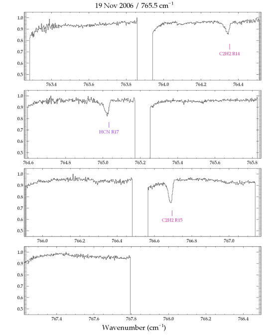
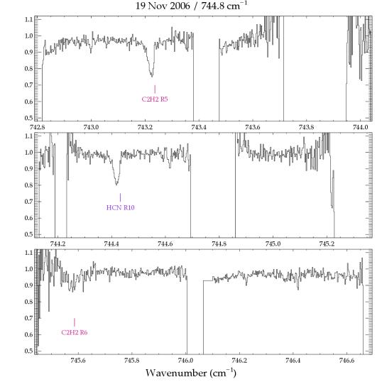
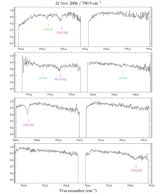
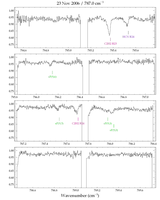
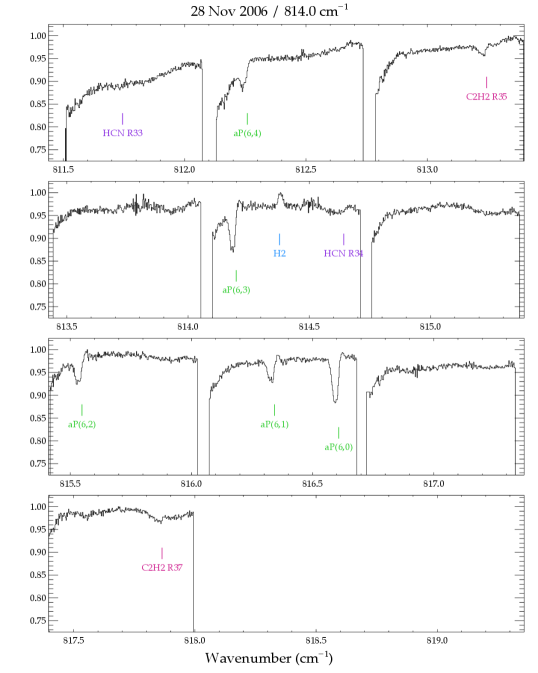
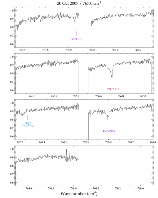
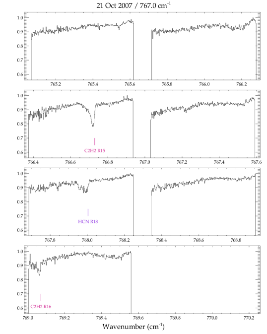
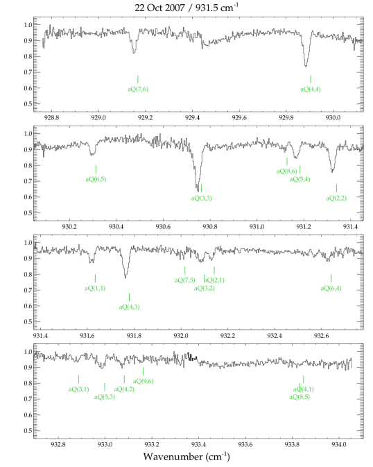
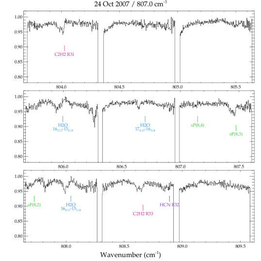
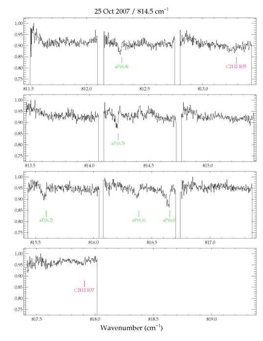
In the TEXES spectra we detect numerous absorption lines of , HCN, and , a few lines of in absorption, and in emission (Table 2). The emission from GV Tau was previously reported in Bitner et al. (2008) and is not discussed further here. Most of the HCN and lines were measured in 2006, with additional lines measured in 2007. The unexpected detection in 2006 of numerous absorption lines was followed up in 2007 with grating settings that probed lower energy transitions. Weak absorption lines of water were also detected in the 2007 spectra. The entire set of pipeline-reduced spectra for GV Tau N are shown in Figure A1. The positions and identifications of the detected lines are indicated.
While the lines are pure rotational transitions within the ground vibrational state, the , HCN, and absorption lines are predominantly ro-vibrational transitions out of the ground vibrational state to a higher vibrational state; the + – line is an exception (see section 3.1).
The HCN vibrational mode is the bending mode. The mode of (HCCH) is the symmetric bending mode, in which the two H atoms vibrate together, and the mode is the antisymmetric bending mode. In the R5 transition, for example, the rotational transition is J=5 to J=6, Q5 is J=5 to J=5, and P5 is J=5 to J=4. For , the H atom spin statistics cause the odd-J (ortho) lines to be three times as strong as the even-J lines, and Q-branch lines are approximately twice as strong as P- and R-branch lines. Since HCN and are linear molecules in their ground vibrational states, only the quantum number J is required to label their rotational states, although the excited bending modes are split into e and f states depending on the relative orientation of the rotational axis and the bending motion.
For , the vibrational mode is the ‘umbrella’ mode in which the three H atoms vibrate together. The ground and states are split by inversion splitting, with lines from the symmetric and anti-symmetric states labelled s and a. For this symmetric top molecule the rotational state is described by two quantum numbers, J (the total angular momentum) and K (the angular momentum about the symmetry axis). Line strengths depend on both J and K, but typically states with K=3n are twice as strong as those with K=3n1. J can change in a radiative transition, but K does not. Transitions are labelled by the lower state J and K.
3.1 HCN and
We detect a total of 8 lines of the HCN band, 14 lines of the band, and one line from the + – band (i.e., absorption out of the vibrational level; Figure A1). In 2006, we detected 12 lines between R5 and R37 and 6 HCN lines between R10 and R34. In 2007, we detected 6 lines between R15 and R37, as well as three HCN transitions (R17, R18, R32) with limits on two additional HCN transitions (R33 and R34). The lower energy levels of the observed lines range from K to K.
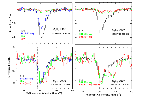
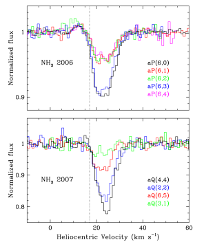
The absorption features range in strength from % deep at high excitation down to a maximum of % deep at intermediate- values (Fig. 1 and Fig. 2). Figure 1 shows representative line profiles of over a range of excitation for 2006 (left) and 2007 (right), both as observed (top) and with the absorption features scaled to the same depth (bottom) in order to compare relative velocity profiles. In the bottom panels, vertical lines indicate the velocity of the gaseous envelope surrounding GV Tau (dashed line; ; or ; Hogerheijde et al. 1998). The MIR molecular absorption is clearly redshifted with respect to the molecular cloud velocity.
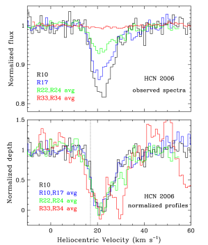
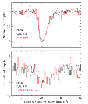
Figure 2 shows the HCN spectra and normalized profiles from the 2006 data; the HCN profiles from 2007 are similar. Figure 3 compares the and HCN profiles for low (top) and high (bottom) excitation lines. The and HCN lines have nearly identical velocity profiles.
At low-, the HCN and lines profiles both have a “single dip” core absorption component centered at 21–22 with a FWHM of , and a red wing extending to (Figs. 1, 2, 3). When scaled to the same depth, the and HCN profiles show a trend in which the red wing becomes stronger (relative to the core) at high (Fig. 1 and Fig. 2), i.e., the high velocity gas is more highly excited or is more optically thick. While low and intermediate rotational levels (e.g., R15 of ) tend to show a wing that smoothly decreases in strength to the red, higher excitation lines show more velocity structure. For example, the R37 line could be fit with velocity components at 21, 28, and 36 . The velocity structure of the (§3.2) and (§S3.3) lines is similar to that seen in the HCN and lines, suggesting that the molecular absorption is composed of multiple velocity components.
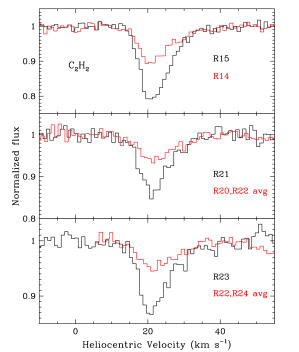
If the absorbing gas is optically thin, the odd- lines should be approximately 3 times stronger than the adjacent even- lines. For several of the stronger lines observed (R14 vs. R15; R21 vs. the average of R20 and R22; R23 vs. the average of R22 and R24), the ratio of the absorption depths of the ortho and para lines is lower, in the absorption core (Fig. 4), indicating that the odd- lines have optical depths of or greater. The relative depths of the neighboring ortho-para lines also differ between the core and the wing. The ratio of the absorption depths declines from within the absorption core to in the red wing beyond 30 (Fig. 4), indicating that the even- lines are also optically thick in the high velocity gas. Interestingly, the observed depths of the lines (%) are far less than expected for optically thick lines. This suggests that the line strengths are significantly diluted, or an intrinsically narrow line is highly broadened by macroscopic motions, or some combination of these two effects.
3.2
We detect a total of 34 lines of the band (Figure A1): 12 transitions in 2006 with lower energy levels from to , and 27 transitions in 2007 with lower energy levels from to . The absorption strengths are similar to those of the and HCN lines and range in strength from % deep for the weakest measured lines to a maximum of % deep for the aQ(3,3) transition measured in 2007. Example spectra for individual lines are shown in Figure 5 for several P-branch lines from 2006 and Q-branch lines from 2007.
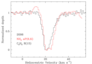
The profiles of the P-branch lines are roughly similar to the and HCN profiles, although there are differences in detail. Figure 6 compares the R15 line () with the average of four aP(6,K) lines from 2006 (). Like the HCN and line profiles discussed in the previous section, the P-branch line profiles also have an absorption core at and a red wing extending to . However, the shape of the core is more square bottomed, with a small shift in the velocity of the blue edge. In addition, the aP(6,K) lines from 2006 show weak emission blueward of the absorption. A similar emission component is not seen in the line profiles of the other molecules, nor in the profiles of other lines (including the aP(6,K) lines from 2007); however, the latter could be due to lower signal-to-noise of the other spectra. Similar line profiles are predicted in radiative transfer models of disk atmospheres with modest radial flows (see Section 4.2).
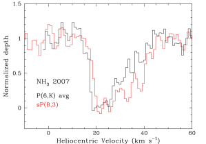
Similar to and HCN, the higher velocity red wing of the profiles becomes stronger, relative to the core, for higher excitation lines. Figure 7 compares the average 2007 profile of the aP(6,K) lines () with that of the sP(8,3) line (). The higher energy line clearly shows enhanced absorption at higher velocities in the red wing.
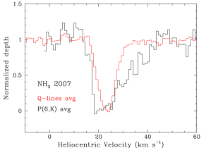
Perhaps surprisingly, the Q-branch lines show the core absorption component (FWHM ) but lack the red wing. Figure 8 compares the average 2007 line profiles of the Q-branch () and aP(6,K) lines. The profile shapes differ markedly, with the higher velocity absorption in the red wing absent in the Q-branch lines. The average Q-branch profile is sharper and centered more to the red than the flat-bottomed P-branch lines. However, the Q-branch profiles also vary with line strength (see Fig. 5, bottom), with the weaker Q-branch lines closer in shape and velocity to those of the aP(6,K) lines. The absence of the red wing in the Q-branch lines may have something to do with the fact that the Q-branch transitions overlap the 10 silicate absorption feature, while the measured P-branch lines fall between 12 and 13 . Detailed radiative transfer models that include these opacity differences may be able to help us understand the origin of the differences in the profiles.
3.3
We detected 4 high excitation lines of in the 2007 spectra (Figure A1), with lower energy levels ranging from 2631 to 3211 . All of the lines are very weak, 2–3% deep. In contrast to the , HCN, and lines, which have a prominent absorption core at , the absorption is deepest at .
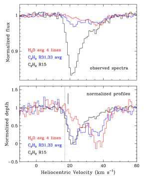
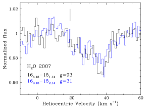
Figure 9 compares the average spectrum and profile of the four detected lines with spectra and profiles of high-excitation (average of R31 and R33) and low-excitation (R15) lines of in the 2007 data. The comparison shows that the absorption profile is strongest in the far red wing of the low- absorption profile. The absorption is very weak in the region of the the 22 component and intermediate in strength at The profile of the higher energy line, whose overall strength is weak, like the absorption, is intermediate between the two profiles: it has the same velocity components as (at roughly 22 , 28 , and 36 ) but with more equal depths.
Figure 10 compares the profiles of the 163,13–152,14 and 164,13–151,14 water lines, which are an ortho-para pair; they have nearly identical Einstein A-values and lower level energies (Table 2) but differ by a factor of 3 in their statistical weights. The absorption strengths of the two transitions are essentially the same, which shows that the absorption is optically thick. At the same time, the absorption depths are very small, which implies that the absorption is highly diluted, either because the absorber covers a small fraction (filling factor) of the background continuum and/or an intrinsically narrow, deeper absorption feature is broadened by macroscopic motions. A similar, but less extreme, result was found for the absorption.
Table 2 lists 4 the detected water lines as well as an additional 4 undetected water lines that were used to constrain the properties of the water absorption.
3.4 Variability
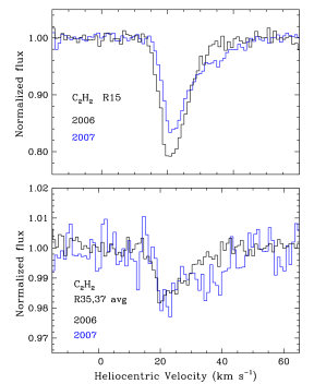
There are some differences in the absorption strength and velocity profiles of the lines observed in 2006 and 2007. Figure 11 compares the 2006 and 2007 spectra of for the R15 line and the average of two high excitation lines. In 2007 the core of the R15 line decreased in strength, while the red wing has increased. In the high excitation lines, the wing also increased in strength in 2007 while the 22 core remained about the same. The same behavior is seen for HCN. The increase in the depth of the red wing relative to the core is common to all transitions and to all three molecules, including the P-branch lines observed in both epochs.
A more subtle change is a small redward shift in the blue edge of the lower excitation and HCN lines, resulting in a change of the line centroid from 22 to 23 . These velocities differ from the average velocity of 19 that Doppmann et al. (2008) found for the 3 HCN lines, in spectra with 13 resolution that did not resolve the line profiles. Hence, velocity variations may be common, but the TEXES data show that this can be produced by changes in the velocity structure of the absorption, rather than just a simple velocity shift of the entire profile.
3.5 Equivalent Widths and Absorption Properties
The equivalent widths (EWs) of the absorption features were used to infer the temperatures and column densities of the absorbing molecules. Because there are differences in absorption strengths and profiles between 2006 and 2007, the EWs measured in the two epochs were analyzed separately.
As noted in previous sections, the “core” and “wing” components of the line profiles show different behaviors as a function of line excitation energy, both in the observed ortho-para ratio of absorption depths and in the interesting absence of a red wing in the Q-branch lines. We therefore measured and analyzed the absorption as that of two velocity components, simply defined: one redward of and the other blueward of the same velocity. A possible alternative would have been to decompose the profile into two Gaussians. However, because the profiles are not strictly Gaussian, and they in fact appear to be composed of multiple components with possibly complex behavior, we adopted the simpler approach, with the goal of capturing the essence of the difference between the lower and higher velocity absorption.
The measured EWs for the two velocity components and their combined EW are given in Tables 3 and 4 for all lines measured in 2006 and 2007, respectively. The uncertainties include both the spectral pixel-to-pixel noise, which comes from the continuum signal-to-noise, and an estimate of the uncertainty in the continuum placement. The average line depth over the velocity interval is also listed for both components. In analyzing the detected absorption, we found it useful to also include upper limits on a few additional lines that could become detectable at very high column density and lower temperatures. These lines are listed in Table 4 along with their 2- upper limits on EW for the high-velocity component.
In the case of a uniform absorbing medium that lies in front of an opaque continuum source, the absorption equivalent width, which is a simple function of the line optical depth can be diluted by unobscured continuum emission (e.g., if the absorber does not completely cover the background MIR continuum source) and/or by emission from the absorber. That is, if the emission from a background source with temperature is absorbed by a medium with opacity and source function , the emergent intensity is
| (1) |
at a frequency in the line and in the neighboring continuum. The fractional intensity decrement in the line relative to the continuum is then
| (2) |
and the equivalent width
| (3) |
where the quantity
| (4) |
combines the effects of the covering fraction of the absorber and the average dilution by emission from the absorber across the line In LTE, where is the temperature of the absorbing medium. However, as a result of the high critical density for vibrational LTE, the vibrational temperature may be less than and both and can be affected by the radiation field.
Here we model the absorbing gas as a uniform slab. The line optical depths are determined by the gas temperature (), and the ratio of the column density of the molecule () to the intrinsic line width, which includes thermal and microturbulent components. If the absorption is approximated as a Gaussian line profile with FWHM , the line center optical depth is
| (5) |
where is the wavenumber of the transition, is the multiplicity of the upper state, is the energy of the transition, is the partition function, and the factor 1.0645 relates the product of the FWHM and peak height of a Gaussian to its area. All of the molecular parameters and data for the partition functions are from HITRAN (Rothman et al 2013; Fischer et al. 2003). We assume that the lower energy levels are in LTE.
For each molecule and velocity component, we plot a curve-of-growth (COG) as ln(EW) versus the logarithm of a quantity proportional to and then determine the model parameters that minimize . The first two parameters, and , determine the line optical depths and the shape of the COG; equivalently, these two parameters set the relative EWs of the lines. The third parameter in this approach, , is a scaling factor that best matches the absolute EWs for all lines. From these three parameters, the value of automatically follows.
Note that and are not independently determined, although it is possible to place physical limits on (and hence ). If all lines are optically thin (all points fall on the linear part of the COG), is not constrained and the only determined parameters are and . The results from the COG analysis are given in Tables 5 and 6. The parameter uncertainties represent 1-, i.e., a 68% confidence interval, where the joint confidence region for the parameters is the space enclosed by the surface of constant that corresponds to the confidence level and the number of free parameters. Note that there is correlation between parameters, such that the upper bound on temperature generally corresponds to lower column density and larger intrinsic line width, and visa versa. The uncertainties depend on the number of lines used, the signal-to-noise of the EWs, and the range in optical depth and lower energy level covered by the measured transitions.
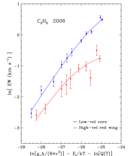
In Figure 12, example COGs are plotted for both the low- and high-velocity components of from 2006. The COG analysis shows quantitatively the conclusion reached from visual examination of the spectra; the high-velocity (HV) component (the red wing) has a higher optical depth than the low-velocity (LV) component (the 22 core), as indicated by the greater curvature in its COG. The line with the highest opacity is the R15, which has an optical depth of 2 for the LV and 6 for the HV component. Remarkably, the temperatures of the HV and LV components are about the same, K. Thus, our finding that higher rotational transitions are more prominent in the HV component is not due to a higher temperature for the high-velocity gas but to greater optical depth (larger ).
Despite its higher optical depth, the EWs and absorption depths of the HV component are smaller than those of the LV component, indicating a larger dilution factor. Because the LV and HV components share the same temperature (Tables 5, 6), the contribution of line emission by the warm absorber to the value of (through the quantity in eq. 1) is the same for both components. Thus, the greater dilution of the HV component (i.e., smaller ) compared to the LV component indicates that the covering fraction of the background continuum is smaller for the high-velocity gas than the low-velocity gas.222Small values of reflect small covering fractions rather than significant emission from the absorbing gas. The vibrational temperature of the absorber and the temperature of the background continuum would have to be very similar for emission to have a significant impact. In LTE, is the same as the rotational temperature of the absorber, which is here K. For =450 K, reducing to 0.16–0.21, the range of dilution factors inferred for the LV component (Tables 5 and 6), requires a background continuum temperature of =480–490 K. Such similar foreground and background temperatures seem implausible; with temperatures that similar, the foreground gas is as likely to produce emission as absorption.
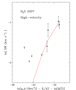
For , the absorption is dominated by the HV component (Section 3.3); the observed redward velocity of the absorption shifts it out of the telluric water absorption, enabling its detection. The component is clearly detected in the average spectrum (Fig. 9), but it is too weak in individual lines to be useful in determining the absorption parameters. Therefore, the analysis was restricted to the HV component. Furthermore, because all four of the detected lines are optically thick, we are unable to constrain the absorption properties using these lines alone. We therefore also included in the analysis the upper limits on several additional water lines covered by our spectra. Because these additional lines, shown in Table 4, would become strong enough to detect at very high column density and/or low temperature, including their upper limits places an upper bound on the water column density. The 2- upper limits were included in the fit using the approach discussed in Sawicki (2012). The best-fit COG for the absorption is shown in Figure 13. The resulting analysis yields the best-fit properties shown in Table 6.
Using the above procedure, we derived gas temperatures of K for both velocity components of all molecules, with one clear exception discussed below. For molecules other than water, the derived values for are in the range , with the value for the HV component consistently 3–7 times greater than that for the LV component. For the HV component of water, is much larger, .
Because radiative transitions between rotational levels of are forbidden, collisions will control the rotational populations in the ground vibrational state. Therefore, LTE should be a good approximation for and the derived temperature a measure of the gas kinetic temperature. For HCN, the critical densities for our measured transitions range from . The derived excitation temperature is the same as that of (for the 2006 data), indicating that the gas densities are at least this high. The measured rotational levels for have comparable critical densities. However, the critical densities for the measured water lines are higher, Models of disk atmospheres predict that warm molecules are present at high densities (), making LTE a reasonable assumption (e.g., Bruderer 2014; Najita & Ádámkovics 2017).
To determine the line-of-sight column density from the constrained quantity requires an assumption about the local line broadening A lower limit on comes from assuming that the local line broadening is thermal, which for the observed molecules is at 450 K. For an upper limit to we can adopt for the observed width of the absorption component (), which would be appropriate if the absorbing medium is highly turbulent. However, this is unlikely, because the profiles of the R15 and R14 lines of are identical across the LV component, i.e., the ortho-para ratio and hence the optical depth is nearly constant across the LV core of the lines. If the absorption was due to a single intrinsically broad () profile, then the optical depth would be highest at the absorption minimum and decrease away from line center, in contrast to the observed profiles.
More likely, the observed width of the absorption feature is produced by multiple lines of sight through the rotating disk atmosphere that pass through gas at different velocities. In this case, the local line broadening is substantially less than the full observed width, implying a smaller line-of-sight column density. In Tables 5 and 6 we list values for for an assumed width of a value between the approximate thermal width of hydrogen () and that of water () at the temperature of the absorption (450 K), implying some amount of microturbulent broadening for the observed molecules. We interpret these values of in the next section.
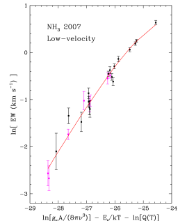
Although we find a K temperature for the velocity components of almost all molecules, we derive a much lower temperature for in 2007 (250 K) than in 2006 (455 K) for the LV component. Because the addition of the Q branch in the 2007 data adds a large number of lines, which cover a greater range in optical depth, the temperature from the COG is well constrained. Setting the temperature to 250 K for the 2006 data gives a extremely bad fit. One could be concerned that the Q branch probes different gas, given its different behavior, i.e., the absence of the red wing in the Q-branch lines. In Figure 14, we plot the COG for the 2007 LV component, where the model COG is the best fit to the combined Q- and P-branch lines. The P-branch lines are plotted with a different color, and follow the same trend as the Q-branch lines. In addition, fitting the Q- and P-branch lines separately yields consistent temperatures.
Comparison with Previous Results. We can compare our results for HCN to the findings of Doppmann et al. (2008), who measured the 3 absorption lines of HCN and in GV Tau N at a resolution of 13 using NIRSPEC on Keck. They fit the HCN spectrum with a temperature of 550 K and an HCN column density of , using a microturbulent velocity of 3 (FWHM = 5.0 ). This is equivalent to . Hence, their result is in reasonable agreement with the values we obtained with the MIR lines for the LV component of HCN.
We can also compare the results from our spectrally resolved molecular spectra with the analysis by Bast et al. (2013) of the Spitzer/IRS spectrum of GV Tau. Our study differs from that of Bast et al. in two important ways. Firstly, the TEXES data spatially resolve the N and S components of the binary, whereas Bast et al. did not account for dilution by GV Tau S. Our TEXES observations confirm that the S component lacks MIR molecular absorption, a result similar to that found in -band molecular spectroscopy of GV Tau N and S (Doppmann et al. 2008; Gibb et al. 2007). Secondly, the high spectral resolution of the TEXES data allows us to resolve the profiles and to infer dilution of the line equivalent widths.
For comparison to Bast et al., we use the values from our analysis with = 1, i.e., the column densities we would derive without taking dilution into account. For and HCN, our column densities are somewhat larger, by factors of 1–3, than those reported by Bast et al. The temperature for HCN is in agreement, but their temperature for (720 K) is higher. For , our values of are similar to the upper limit reported by Bast et al. ( for 500 K). All of our derived column densities would be larger for . Some of the observed differences may be due to variability, because the Spitzer and TEXES data were taken at different times.
To summarize, the TEXES spectra reveal warm (), redshifted MIR molecular absorption in GV Tau N, with larger column densities than inferred in previous studies. The HV component of the absorption is more optically thick than the LV component, has a column density 3–6 times larger, and is more highly diluted (by a factor ) than the LV component due to a smaller covering fraction of the background MIR continuum.
4 Discussion
4.1 Origin of the Absorption
The working hypothesis in the literature is that the molecular absorption in GV Tau N occurs in gas in the disk atmosphere observed against the hotter dust continuum from smaller radii in a disk viewed close to edge-on (Gibb et al. 2007; Doppmann et al. 2008; Bast et al. 2013). Here we discuss the origin of the absorbing gas in light of our results on the temperature, column densities, and line profiles of the molecular absorption.
Clues from Temperature and Column Density. We find that the absorbing gas is warm ( K) and the detected molecular species show profiles that can be modeled as multiple velocity components that probe gas along the same lines of sight to the 12 continuum. The rotational temperatures derived for the HCN, , and absorption are similar to (but at the cool end of) the excitation temperatures derived for the same molecules from the MIR molecular emission observed from T Tauri disks (400–1000 K; Carr & Najita 2011; Salyk et al. 2011). The latter is thought to arise from the heated disk atmosphere within an au of the star (e.g., Najita et al. 2011; Najita & Ádámkovics 2017).
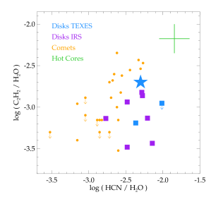
The relative column densities of the molecular species detected in absorption in GV Tau N are also consistent with the ratios derived for the MIR molecular emission from T Tauri disks. For the high-velocity absorption component measured for GV Tau N in 2007, for which a column density could be determined, the column density ratios are = 0.002, = 0.005, and = 0.4. Figure 15 compares the GV Tau N column density ratios (blue star) with the emission column density ratios of T Tauri disks derived from high and low resolution spectra (squares). The GV Tau N values are similar to the ratios derived from T Tauri star emission spectra using slab models that make assumptions similar to those adopted here. The similar column density ratios are consistent with the interpretation that the GV Tau N absorption arises in a disk atmosphere.
At the same time, the absolute column densities of the MIR absorption are much higher than the column densities seen in emission. Here we compare specifically to results for AS205 N and DR Tau, two high accretion rate disks viewed at low inclination. As the only sources whose HCN and emission has been measured at high spectral resolution, their velocity-resolved spectra enable tighter constraints on the properties of the emitting gas (Najita et al. 2018). For a valid comparison (apples to apples), we assume thermal local linewidths for the GV Tau N absorption, as assumed in the earlier emission line analysis. The column densities of , HCN, and in the HV absorption component of GV Tau N are 40 times greater on average than the emission column densities of AS205 N and DR Tau, and the (HCN and ) column densities of the LV component of GV Tau N are times greater. The roughly order-of-magnitude larger line-of-sight column densities observed in absorption vs. emission are expected if the warm molecular layer responsible for the T Tauri star emission is viewed at high inclination in GV Tau N, as in an edge-on disk.
There is little definitive information available on the orientation of the GV Tau N disk. Modeling of MIR interferometric observations made with VLTI/MIDI favored a high inclination for GV Tau N ( degrees; Roccatagliata et al 2011). In addition, the CO overtone emission from the inner disk of GV Tau N is broad () suggesting the disk is not close to face on (Doppmann et al. 2008). In contrast, modeling that fits the spectral energy distribution (SED) and scattered light images of GV Tau N with a disk + envelope model favors a lower inclination ( degrees; Sheehan & Eisner 2014). However, the SED modeling may not provide a strong constraint on the orientation of the inner disk of GV Tau N; because the modeling weights large-scale phenomena prominently in the fit, the preferred solution may be influenced primarily by the envelope properties rather than the inner disk ( au) properties where the warm absorption arises.
Clues from Line Profiles. While the results above echo previous results from the literature, the high velocity resolution of the TEXES data lends new insights into the dynamics of the absorbing gas. The =600 Spitzer spectra detected molecular bands but did not resolve individual lines. The NIRSPEC/Keck spectra studied by Doppmann et al. (2008) and Gibb et al. (2007) marginally resolved individual HCN lines in the -band. In comparison, the TEXES data, with a resolution of measure the profiles of individual lines.
In interpreting the line profiles, we adopt as the system velocity for GV Tau N the velocity measured for the gaseous envelope surrounding GV Tau ( or ; Hogerheijde et al. 1998). The stellar radial velocity of GV Tau N is not well known. One estimate, based on an absorption component detected in the CO overtone emission from the source (), is blueshifted relative to both the cloud and envelope velocity, suggesting that the central source may be a spectroscopic binary (Doppmann et al. 2008).
As described in Section 3, the GV Tau N line profiles have single-dipped, FWHM absorption line profiles; the absorption core has a velocity offset redward of the system velocity and a red wing extending to higher velocities. The redward offset of the core and red wing are not expected for a simple rotating disk and suggests gas that is radially inflowing. The redshifted absorption we observe is reminiscent of earlier Keck/NIRSPEC results for GV Tau N. Doppmann et al. (1998) found that the NIR HCN absorption toward GV Tau N, centered at is redward of the system velocity.
Assuming that all of the absorbing gas resides at , Doppmann et al. (2008) argued that the NIR warm molecular absorption is unlikely to arise from gas in an infalling envelope. Given the inferred mass of the stellar component(s) of GV Tau N (), the envelope infall velocity would reach the observed velocity shift at a distance of 360 au. In contrast, models of infalling protostellar envelopes predict that the gas temperature reaches 500 K only within 2 au of the star at the accretion luminosity of GV Tau (Ceccarelli et al. 1996, their Fig. 4), i.e., well within the distance of 360 au that would be inferred for the infalling gas based on its velocity relative to the molecular envelope. If the NIR molecular absorption arises in infalling gas at 360 au, an additional, non-traditional source of heating is need to explain the observed temperature of the absorbing gas.
A similar argument applies to the MIR absorption. At the higher resolution and signal-to-noise of the TEXES spectrum compared to the NIRSPEC results, we find that the core of the MIR molecular absorption, centered at 21–22 , is redward of the system velocity, with the red wing of the absorption extending to larger velocities, redward of the system velocity. Infalling gas would reach the redshifted velocity of the absorption core at au and the wing velocity at au from an star. While some of the high velocity gas (arising within au) might be warm enough to explain the observed absorption, the bulk of the infalling gas at au would be too cool to explain the observed absorption.
Moreover, because of angular momentum conservation, it may be very difficult for infall to reach the inner few au of a Class I system. For rotating infall, angular momentum prevents direct accretion onto the star and its vicinity, instead causing the infalling material to reach the disk near the centrifugal radius (20–40 au). The difficulty of reaching the inner few au through infall is even more true for late accretion sources in which the infall is increasingly dominated by high angular momentum material. GV Tau, which has a weak molecular envelope, is such a late accretion source, i.e., transitioning from a Class I source to a Class II source.
Another general argument against infall (and in favor of an inner disk atmosphere) is the molecular composition of the absorption and its rarity. Figure 15 shows that the GV Tau ratios of , HCN, and water are similar to those of T Tauri disk atmospheres seen in emission. Such absorption is rare. GV Tau N is the only Class I source known to show , HCN, water, and in absorption. One other source shows and HCN absorption in its Spitzer spectrum (IRS46; Lahuis et al. 2006).
If the temperature and composition we observe in GV Tau N were typical of infalling envelopes, we would commonly observe these features in Class I sources. Compared to a disk atmosphere, gas in an infalling envelope would cover a much larger fraction of the star, approximately the range of polar angles between the disk surface and the inner cavity carved out by outflow. As a result, absorption from infall would be detected over a much wider range of viewing angles than disks viewed nearly edge on. The rarity of molecular absorption like that seen in GV Tau N argues against its origin in an infalling envelope.
Disk Origin. Unlike the infalling envelope scenario, a nearly edge-on rotating disk can account for almost all of the properties of the observed molecular absorption: the temperature and column density (as discussed above) and its line width. Single-dipped absorption line profiles can arise when a disk atmosphere is seen in absorption against the MIR continuum arising from smaller radii. While both the line absorption and the continuum emission likely arise over a range of radii, for simplicity in the discussion below, we assume that the continuum arises from a compact region and the absorption occurs at larger radii . Because the MIR continuum is compact compared to , only the portion of the disk atmosphere at that is close to the line-of-sight to the continuum is seen in absorption, i.e., within an azimuthal angle where (Fig. 16)
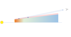
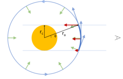
Gas at along the line-of-sight to the MIR continuum has a maximum projected radial velocity of where is the disk rotational velocity at and is the disk inclination. For a disk in Keplerian rotation, where the projected radial velocity due to rotation at is and the projected radial velocity at is If the 12 continuum arises within au of the star, where for an star, maximum absorption velocities of would arise at a modestly larger radius of au (That is, gas at this radius would absorb background continuum emission from au over the FWHM of the observed absorption features.) Higher velocity absorption would arise from gas at smaller radii. Lower velocity absorption arises from both gas at larger radii as well as gas at smaller radii that are close to the line of sight to the star. At a disk radius of 4 au, the maximum absorption velocity would be
Thus, a conventional rotating, edge-on disk can account for almost all of the properties of the observed molecular absorption (the temperature, column density, and its line width), except for its redshift from the system velocity. We can also account for the redward offset of the absorption core if the gas in the disk atmosphere is also radially inflowing along the disk surface (Fig. 16). Such “surface accretion” flows are found in simulations of rotating magnetized disks.
4.2 Surface accretion in GV Tau N?
In their global ideal MHD simulations of thin disks threaded by a vertical magnetic field, Zhu & Stone (2018) found that accretion occurs primarily in a surface accretion flow in the upper, magnetically dominated disk surface. (See also earlier theoretical work by Stone & Norman 1994; Beckwith et al. 2009; Guilet & Ogilvie 2012, 2013.) The accretion is supersonic, reaching inward velocities –4 where is the sound speed.
In their simulation, the rapid accretion at the disk surface (primarily due to the magnetic stress) carries the magnetic field inward, pinching it inward at the disk surface. As a result, the disk atmosphere is connected magnetically to the midplane at larger radii, which spins down the atmosphere, producing significantly sub-Keplerian rotation—as small as 60% of Keplerian rotation—in the atmosphere. The inward pinching of the magnetic field also launches a disk wind, although the torque due to the wind at the disk surface plays only a small role in driving accretion.
The expected properties of the accreting atmosphere are roughly consistent with the observed properties of the molecular absorption in GV Tau N. For molecular gas at 500 K, supersonic accretion at –4 corresponds to –5 km/s, qualitatively similar to the redshift of the absorption core ( km/s); the velocities of the red wing (–20 km/s) correspond to higher velocities . For gas in sub-Keplerian rotation at a disk radius along the line of sight to the MIR continuum (which arises within ), its projected radial velocity spans the range , as described above, where is a factor that accounts for possible deviations from Keplerian rotation. If and au so that for a stellar mass of , an observed absorption core with a FWHM of would correspond to absorbing gas at au
Preliminary work on a detailed radiative transfer model of a rotating disk with radial inflow, viewed nearly edge on, appears to be able to account for the properties of the molecular absorption observed in the GV Tau N spectrum. The modeling, which builds on the previous results of Lacy (2013), can plausibly account for the shape of the absorption components as well as the slightly blueshifted emission seen in the P-branch profiles. In one promising scenario, rapidly inflowing gas near the inner rim of the disk is seen against the continuum from the inner rim, and more slowly inflowing gas located near the disk surface at larger radii is seen against the disk continuum at smaller radii (Lacy et al., in preparation).
If the observed absorption arises in a surface accretion flow, the flow may carry a significant mass accretion rate. For an inward flow with velocity and vertical column density at a characteristic radius , the mass accretion rate is
| (6) |
If we assume
| (7) |
where is the observed line-of-sight molecular absorption column (e.g., values in the final column in Tables 5 and 6), is the ratio of the vertical to the line-of-sight molecular column densities, and is the abundance of the tracer molecule relative to hydrogen, the associated accretion rate is
| (8) |
For the observed HCN absorption, the properties of its LV component are , Assuming an abundance in the warm disk atmosphere of at au, as found in disk chemistry models that account for the MIR molecular emission properties of T Tauri disks (Najita & Ádámkovics 2017), and , the corresponding vertical column density and accretion rate are and
Similarly, given the inferred properties of the HV HCN absorption component, , the corresponding vertical column density is and the accretion rate associated with the HV component is 20 times larger than that of the LV, or Using the properties of the HV water absorption () and a conservative water abundance estimate of (Najita & Ádámkovics 2017) yields a similarly large estimate of the accretion rate of the HV component,
In adopting abundances for this estimate, we want to select values from model atmospheres that are able to match the properties of the Spitzer molecular emission from inner disks and use abundance values appropriate for the warm atmosphere region that is responsible for the emission. The models in Najita & Ádámkovics (2017) do a fair job reproducing the properties of many of the molecules detected with Spitzer. To make a conservative estimate of the accretion rate, we have adopted model abundances at the high end of the predicted values within the layer responsible for the emission. The properties of the Walsh et al. (2015) and Woitke et al. (2018) models differ from those of Najita & Ádámkovics in detail (e.g., the molecular atmosphere of Woitke et al. is much cooler), but their model abundances, if adopted, would imply similar or larger accretion rates. For example, Walsh et al. find a peak HCN abundance of which would imply a much larger accretion rate for the LV component of The peak water abundances for all of the models are similar Thus, the molecular abundances of current disk atmosphere models suggest large accretion rates for both the LV and HV components.
The assumed value of is plausible for the geometry of a highly inclined disk viewed close to edge on. A more accurate value could be obtained from a more complete model of the physical, thermal, and chemical disk conditions.
The above discussion assumed a local line broadening of (Tables 6 and 7) and that the full absorption width we measure is actually the result of observing absorption along multiple lines of sight through the rotating disk atmosphere, encountering gas at different projected velocities. The column densities and accretion rates above would be smaller by a factor of two, or larger by a factor of 4, if we assumed that the local line broadening is instead thermal width or the full observed width of the absorption component, respectively.
The resulting vertical column densities ( for LV; for HV) are similar to and larger than the vertical column densities thought to be responsible for the emission from T Tauri disks. The resulting accretion rates ( for LV; for HV) span the range observed from typical to very active T Tauri stars. While there are substantial uncertainties associated with the above estimates (including the fact that we only measure gas columns where the molecular tracers are abundant and atomic gas is not probed), the inferred accretion rates are substantial and fall within the expectations for T Tauri stars. Thus, the observed radial inflow does appear capable of explaining the observed accretion rates of very active T Tauri stars and Class I objects.
The idea of accretion at the disk surface dates back at least to Gammie (1996), who described a “layered accretion” picture of T Tauri disks, in which only the surface region of the disk that is sufficiently ionized to couple to magnetic fields participates in accretion via the magnetorotational instability (the “active layer”), and the deeper layers of the disk are a non-accreting “dead zone.” In Gammie (1996), the active layer was thick, and an equivalent viscosity parameter was sufficient to account for observed T Tauri stellar accretion rates (). In the intervening years, more detailed models of disk ionization and our improved understanding of the role of non-ideal MHD processes have shrunk theoretical expectations for the vertical extent of the accreting layer to smaller and smaller column densities, requiring larger equivalent values of and larger inflow velocities to deliver the same accretion rate. Here T Tauri-like accretion rates appear to be transported over vertical columns of only
Supersonic surface accretion flows—which differ from previous disk accretion mechanisms in that accretion is driven not by turbulence or a wind, but primarily by large-scale net magnetic fields in the disk atmosphere (Zhu & Stone 2018)—may help resolve the open question of how protoplanetary disks accrete at planet formation distances (0.3–10 au). Because of the low ionization fractions of disks below their surfaces, it is increasing unclear whether turbulence generated by the magnetorotational instability (MRI) can drive a significant accretion rate in protoplanetary disks (e.g., Turner et al. 2014).
The apparent evidence for a supersonic surface accretion flow in the disk of GV Tau N suggests an alternative pathway for disk accretion. As a mechanism that redistributes angular momentum within the disk rather than removing it from the system—as in a disk wind—the supersonic surface accretion flows studied by Zhu & Stone (2018) contribute to disk spreading: angular momentum from the disk surface is transported to the midplane at larger radii, which induces the surface to accrete and the midplane to spread to larger radii. As an “in-disk” transport mechanism, such surface accretion flows may help explain the larger sizes of gas disks surrounding Class II sources (as large as au) compared to those of Class I sources (typically au). The striking size difference has been interpreted as evidence that some “in disk” angular momentum transport process is active in the Class II (T Tauri) phase (Najita & Bergin 2018).
Our results may also be related to magnetothermal wind-driven accretion. Because the winds rely on relatively weak magnetic fields, their magnetic lever arms are small; as a result, transporting disk material from large radii to small (over a factor of 30 in radius, from 10 au to 0.3 au) is an inefficient process requiring large wind mass loss rates, comparable to or greater than the accretion rate (Bai & Stone 2013). Although strong observational evidence for such massive, angular momentum-removing disk winds is currently lacking, the winds are also predicted to produce accretion in narrow current sheets, which can reach high velocities near the disk surface under certain conditions (Bai 2013). If the net vertical field is anti-aligned with disk rotation, near-sonic to supersonic inflow can develop on one side of the disk surface over some range of radii; under other conditions, the accretion flow reaches much lower velocities or occurs close to the midplane (Bai & Stone 2013, Bai 2017). The accretion flow we observe in GV Tau N may be related to the predicted high-velocity flows.
Thus, our spectroscopic results appear to capture disk accretion in action and provide observational support for supersonic surface accretion, a potentially important mode of accretion in protoplanetary disks. To explore this possibility further, we need future spectroscopic searches for redshifted warm molecular absorption from other Class I sources; the incidence rate of the absorption, which constrains its covering fraction, can distinguish between an origin in a disk atmosphere (small covering fraction) or an infalling envelope (large covering fraction). Detailed radiative transfer (RT) modeling is needed to understand whether the line profiles we observe can actually be produced in disk atmospheres undergoing surface accretion. Similarly, thermal-chemical-RT modeling of infalling envelopes is needed to explore that alternative scenario as an explanation for the observed line profiles.
In addition, future theoretical work is needed to understand whether surface accretion flows can be driven under realistic ionization conditions in protoplanetary disks; the Zhu & Stone (2018) simulations were carried out assuming ideal MHD. At the observed inflow velocities of , the accreting material will travel an au in a year, implying that the flow must be rapidly replenished in order to sustain it over protostellar lifetimes ( yr). Whether and how the replenishment occurs—from disk inflows at larger radii and/or from deeper in the disk—is an open question. The results reported by Fuente et al. (2020) may provide a clue. They find evidence for redshifted absorption at modest inflow velocities () in cool molecular gas at larger distances from GV Tau N, as traced in 13CO (J=3-2).
It would also be useful to obtain additional observational evidence for surface accretion flows. As discussed above, even if disks do commonly accrete through their sub-Keplerian surfaces at supersonic speeds, such flows are unlikely to be commonly observed. Nearly edge-on disks, like that inferred for GV Tau N, are advantageous systems in which to search for surface accretion flows because the modest inward motions (few times the sound speed) are more readily detected from that viewing angle. However, edge-on disks are intrinsically rare because of their special orientation. Consistent with this picture, GV Tau N is one of the few YSOs to show molecular absorption in Spitzer/IRS spectra, and yet its SED is similar to that of other Class I sources (Furlan et al. 2008). That is, GV Tau N appears to be a typical Class I source viewed at an unusual inclination.
Although GV Tau N is rare in its molecular absorption properties, radial inflows have been reported in several other disk systems. As described by Zhang et al. (2015), the classical T Tauri star AA Tau, whose inner disk is highly inclined (–75 degrees), shows very broad CO fundamental emission lines, with narrow absorption superposed near the line center. Following a photometric dimming event in 2011, the molecular absorption component increased in strength and showed a constant redshift of with respect to the star. The observed velocity shift, temperature of the absorbing gas ( K), and inferred column density of the absorber () are comparable to the properties of the absorption in GV Tau N.
Perhaps most dramatically, Boogert et al. (2002) reported redshifted absorption in the 5 CO absorption spectrum of the Class I protostar L1489 IRS. The CO spectrum revealed redshifted absorption profiles similar to those seen here, but with a red wing extending to produced by warm ( K) gas. The absorption was interpreted as inward flowing gas at the warm disk surface, although at the time the phenomenon was reported, the physical origin of the gas was unclear. It is tempting to speculate that the CO absorption in L1489 IRS also arises in a disk surface accretion flow, albeit one with a very high inflow velocity.
As another possible example of a surface accretion flow but on a larger scale, spatially resolved CO =3–2 imaging with ALMA of the Herbig Ae star HD100546 shows deviations from Keplerian rotation which have been interpreted as indicating either a severely warped and twisted inner disk or radially infalling gas within 100 au (Walsh et al. 2017). The lack of evidence for a disk warp from high contrast imaging of the dust disk favors the latter explanation. To explain the CO spatial and spectral structure, the required inward velocities are several times the sound speed, similar to the inflow speeds found in simulations that report surface accretion flows (Zhu & Stone 2018). Walsh et al. found reasonable fits to the HD100546 data with a radial flow that is 63% of the Keplerian velocity within 84 au. Given the Keplerian velocity of HD100546 at 84 au (assuming a star), the radial flow velocity is If the gas temperature in the disk atmosphere at 84 au is 30 K, the expected inward flow velocity from a surface accretion flow is approximately similar to the radial flow velocity inferred from the observations.
Similarly, ALMA imaging of HCO+ emission from the classical T Tauri star AA Tau has a twist (within the innermost ring at 40 au) in the projected velocity field relative to the velocity field at larger radii, which is also interpreted as a warp or an inward radial flow (Loomis et al. 2017). Thus, although radial inflows have not been much reported to date, studies of detailed disk dynamics with ALMA and high resolution studies of nearly edge-on disks, carried out for larger samples than have been explored to date, can clarify this picture.
Another way to detect surface accretion flows may be through their sub-Keplerian rotation. While disk rotation at planet formation distances ( au) has been demonstrated using velocity-resolved molecular emission line profiles (e.g., CO fundamental emission), demonstrating that the rotation is sub-Keplerian requires spatial constraints on the observed velocities (i.e., spatially and spectrally resolved emission or spectroastrometry; e.g., Pontoppidan et al. 2011) as well as independently determined stellar masses. The latter may be challenging to obtain. One of the “gold standard” methods for measuring pre-main-sequence stellar masses is to spatially resolve the rotation of outer disks assuming pure Keplerian rotation (e.g., Simon et al. 2000).
4.3 First Detection of in an Inner Disk?
Although ammonia has been previously reported in the outer disk of one young star (TW Hya, in data taken with the Herschel Space Observatory; Salinas et al. 2016), it has not been previously reported in inner disks, in either emission or absorption. In their analysis of Spitzer molecular emission spectra taken at low resolution, Salyk et al. (2011) reported upper limits on the column density of ammonia, based on simple slab modeling and an assumed temperature of 400 K. The results correspond to upper limits on the ratio of ammonia to water of [/] . The analysis by Bast et al. (2013) of the Spitzer absorption spectrum of GV Tau led to an upper limit on its absorption column density of assuming a temperature of 500 K. Our measured absorption columns for towards GV Tau N are consistent with these upper limits.
Ammonia upper limits have also been derived from high resolution spectra of inner T Tauri disks. Mandell et al. (2012) reported upper limits on warm emission corresponding to [/] based on VLT/CRIRES spectra at 3. Summarizing the results of a Gemini/TEXES program to search for Q-branch emission at 10.75 from inner T Tauri disks, Pontoppidan et al. (2019) found a lower average abundance upper limit of [/] . When compared with the HCN abundance measured in the same disks, the upper limit corresponds to [/HCN]
Here we find a much larger [/HCN] ratio for GV Tau N, which shows comparable absorption column densities in and HCN. Using the best constrained values, that of for the low velocity component of each molecule at each epoch, our inferred ratio of [/HCN] is much larger than the [/HCN] upper limits obtained by Pontoppidan et al. (2019) from the molecular emission spectrum of three T Tauri disks.
Whereas conspicuous emission is absent in the Spitzer IRS spectra of T Tauri stars (e.g., Salyk et al. 2011, Carr & Najita 2011), detectable emission is expected if is co-located with the HCN (i.e., has the same temperature; K in emission) and has an abundance similar to that of HCN. To illustrate this discrepancy, we show in Figure 17 examples of predicted molecular emission spectra for simple slab models of T Tauri disks. The predictions adopt the HCN column densities that have been derived for these disks assuming that the HCN emission has the same temperature and emitting area as the emission (Carr & Najita 2011; Najita et al. 2018). At the GV Tau N column density ratio of [/HCN]=0.5 and a temperature of 600 K, the resulting emission would be measureable (solid red line). At the lower ratio of [/HCN]=0.1, corresponding to the high-resolution limits from Pontoppidan et al. (2019), the emission would not be detectable (blue line).
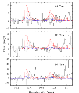
The much higher [/HCN] column density ratio observed in absorption GV Tau N compared to that seen in emission in T Tauri disks might be expected if the emission and absorption features probe the conditions at different disk heights. In their thermal-chemical models of irradiated disk atmospheres, Najita & Ádámkovics (2017) find that is abundant deeper in the atmosphere, and at lower gas temperature, than the region in which HCN and are abundant. Thus, we expect a low [/HCN] ratio in the HCN-emitting gas (Figure 17, blue line). Abundant but cool located below the HCN-emitting gas would also produce weak to negligible emission (Figure 17, dashed red line).
In contrast, cool gas could still be readily detected in absorption in transitions out of the ground vibrational state, particularly with the large slant column densities for a disk viewed at high inclination. The cooler temperatures we measure for the , HCN, and absorption (450 K), compared to the typical temperatures of the HCN and emission from T Tauri stars (600-1200 K; Carr & Najita 2011; Salyk et al. 2011) are consistent with the idea that the GV Tau N absorption probes a deeper layer in the disk atmosphere than the region responsible for the MIR molecular emission from T Tauri disks. The low temperatures we find for the absorption (250 K in 2007 and 450 K in 2006) are roughly consistent with this explanation for the lack of detectable emission from T Tauri disks and with the cooler temperatures anticipated for compared to HCN from the disk thermal-chemical models.
The measured column densities of and HCN in GV Tau N add to our current understanding of the nitrogen reservoir in disks. As described by Pontoppidan et al. (2019), nitrogen is highly depleted in the bulk Earth, by 5–6 orders of magnitude, compared to its cosmic abundance. The low abundance suggests that the bulk carrier of nitrogen in the material that formed the Earth was much more volatile than water, favoring a nitrogen-bearing molecule like N2, which has a low binding energy (430 K) compared to other potentially abundant molecules such as HCN and (3610 K and 3130 K respectively; Walsh et al. 2015). Our results for GV Tau N are consistent with this picture. Because the measured column of is modest, only comparable to that of HCN, it cannot be a major missing reservoir of nitrogen, and a molecule like N2 is instead the likely dominant nitrogen reservoir.
5 Summary and Conclusions
The mid-infrared spectra of GV Tau N reported here were obtained with the original goal of studying the physical properties and molecular content of a disk viewed edge-on. The opportunity to study an unusually large column density of disk gas in absorption offered the potential to detect new molecular species. Consistent with that expectation, the TEXES spectra revealed the first evidence for in the planet formation region of disks. The measured temperatures, molecular column densities, and column density ratios of the detected species (, HCN, , and ) are consistent with the properties of a disk atmosphere within a few au of the star viewed at high inclination. While the abundance measured here is higher than the upper limits obtained from molecular emission studies of disks, our results do confirm the expectation that is not a major missing reservoir of nitrogen. If, as expected, the dominant nitrogen reservoir in inner disks is instead N2, its high volatility would make it difficult to incorporate into forming planets, a situation that may help to explain the low nitrogen content of the bulk Earth.
More interestingly, the TEXES spectra reveal an unexpected and significant redshift to the detected molecular absorption features, indicative of inflow at the disk surface. From the properties of the molecular absorption (column density, velocity shift), we can infer that the redshifted absorption carries a significant accretion rate: comparable to the stellar accretion rates of active T Tauri stars. Thus we may be observing disk accretion in action. The results may provide observational evidence for a new disk accretion pathway for young protoplanetary disks: supersonic “surface accretion flows.” These flows have been found in MHD simulations of magnetized disks (e.g., Zhu & Stone 2018), but their potential role in young protoplanetary disks has received limited attention to date. The observed flows may also be related to accretion flows generated by magnetothermal winds. Future spectroscopy of the dynamics of other edge-on disks would help establish whether supersonic inward flows are common among young disks. In addition, future simulations are needed to understand whether supersonic surface accretion flows can be sustained under realistic ionization conditions in protoplanetary disks.
Appendix A TEXES Spectra of GV Tau N
The figures in this section show the entire set of spectra of GV Tau N used in this study. Each panel shows the pipeline-reduced spectra on the observed wavelength scale before additional corrections were made to remove low-order structure in the continuum. Detected lines are annotated at the velocity of the gaseous envelope surrounding GV Tau, (or ; Hogerheijde et al. 1998). The molecular absorption features are clearly redshifted with respect to the envelope velocity.
References
- (1) Bai, X. 2017, ApJ, 845, 75
- (2) Bai, X. & Stone, J. M. 2013, ApJ, 769, 76
- (3) Bast, J. E., Lahuis, F., van Dishoeck, E. F., & Tielens, A. G. G. M. 2013, A&A, 551, 118
- (4) Beckwith, K., Hawley, J. F., & Krolik, J. H. 2009, ApJ, 707, 428
- (5) Bender, C. 2010, in “Astronomy of Exoplanets with Precise Radial Velocities,” workshop at Penn State University, University Park, PA, http://personal.psu.edu/jtw13/rvworkshop/
- (6) Bitner, M. A. et al. 2008, ApJ, 688, 1326
- (7) Boogert, A. C. A., Hogerheijde, M. R., & Blake, G. A. 2002, ApJ, 568, 761
- (8) Brittain, S. D., Rettig, T. W., Simon, T., Kulesa, C. 2005, ApJ, 626, 283
- (9) Bruderer, S., Harsono, D., & van Dishoeck, E. F. 2015, A&A, 575, 94
- (10) Carr, J. S., & Najita, J. R. 2008, Science, 319, 1504
- (11) Carr, J. S., & Najita, J. R. 2011, ApJ, 733, 102
- (12) Ceccarelli, C., Hollenbach, D. J., & Tielens, A. G. G. M. 1996, ApJ, 471, 400
- (13) Davis, S., Teasley, T., Brittain, S. D., Doppmann, G., & Najita, J. R. 2015, BAAS, 225, 348.05
- (14) Doppmann, G. W., Najita, J. R., & Carr, J. S. 2008, 685, 298
- (15) Fuente, A., Treviño-Morales, S. P., Le Gal, R., Rivière-Marichalar, P., Pilleri, P., Rodríguez-Baras, M., & Navarro-Almaida, D. 2020, MNRAS, in press; arXiv:2006.15065
- (16) Furlan, E., et al. 2008, ApJS, 176, 184
- (17) Gammie, C. F. 1996, ApJ, 457, 355
- (18) Gibb, E. L. & Horne, D. 2013, ApJL, 776, L28
- (19) Gibb, E. L., Van Brunt, K. A., Brittain, S. D., & Rettig, T. W. 2007, ApJ, 660, 1572
- (20) Guilet, J., & Ogilvie, G. I. 2012, MNRAS, 424, 2097
- (21) Guilet, J., & Ogilvie, G. I. 2013, MNRAS, 430, 822
- (22) Guilloteau, S., Dutrey, A., Piétu, V., & Boehler, Y. 2011, A&A, 529, 105
- (23) Hartmann, L., Herczeg, G., & Calvet, N. 2016, ARAA, 54, 135
- (24) Hogerheijde, M. R., van Dishoeck, E. F., Blake, G. A., & van Langevelde, H. J. 1998, ApJ, 502, 315
- (25) Horne, D., Gibb, E., Rettig, T. W., Brittain, S., Tilley, D., & Balsara, D. 2012, ApJ, 754, 64
- (26) Kruger, A. J., Richter, M. J., Carr, J. S., Najita, J. R., Doppmann, G., & Seifahrt, A., 2011, ApJ, 729, 145
- (27) Lacy, J. H., Richter, M. J., Greathouse, T. K., Jaffe, D. T., & Zhu, Q. 2002, PASP, 114, 153
- (28) Lahuis, F., van Dishoeck, E. F., Boogert, A. C. A., Pontoppidan, K. M., Blake, G. A., Dullemond, C. P., Evans, N. J., II, Hogerheijde, M. R., Jørgensen, J. K., Kessler-Silacci, J. E., Knez, C. 2006, ApJ, 636, L145
- (29) Lee, S., Lee, J., Park, S., Lee, J.-J. Kidder, B., Mace, G. N., & Jaffe, D. T. 2016, ApJ, 826, 179
- (30) Leinert, C., & Haas, M. 1989, ApJ, 342, L39
- (31) Loomis, R. A., Öberg, K. I., Andrews, S. M., & MacGregor, A. 2017, ApJ, 840, 23
- (32) Mandell, A. M., Bast, J., van Dishoeck, E. F., et al. 2012, ApJ, 747, 92
- (33) Najita, J. R., Ádámkovics, M., & Glassgold, A. E. 2011, ApJ, 743, 147
- (34) Najita, J. R., & Ádámkovics, M. 2017, ApJ, 847, 6
- (35) Najita, J. R., & Bergin, E. A. 2018, ApJ, 864, 168
- (36) Najita, J. R., Carr, J. S., Salyk, C., Lacy, J. H., Richter, M. J., & DeWitt, C. 2018, ApJ, 862, 122
- (37) Pontoppidan, K. M., Blake, G. A., & Smette, A. 2011, ApJ, 733, 84
- (38) Pontoppidan, K. M., Salyk, C., Banzatti, A., Blake, G. A., Walsh, C., Lacy, J. H., & Richter, M. J. 2019, ApJ, 874, 92
- (39) Pontoppidan, K. M., et al. 2008, ApJ, 678, 1005
- (40) Rettig, T., Brittain, S.. Simon, T., Gibb, E., Balsara, D. S., Tilley, D. A., & Kulesa, C. 2006, 646, 342
- (41) Roccatagliata, V., Ratzka, T., Henning, T., Wolf, S., Leinert, C., & Bouwman, J. 2011, A&A, 534, 33
- (42) Rothman, L. S., Gordon, I. E., Babikov, Y., et al. 2013, JQSRT, 130, 4
- (43) Fischer, J., Gamache, R. R., Goldman, A., Rothman, L. S., & Perrin, A. 2003, JQSRT, 82, 401
- (44) Salinas, V. N. et al. 2016, A&A, 591, 122
- (45) Salyk, C., Pontoppidan, K. M., Blake, G. A., Najita, J. R., & Carr, J. S. 2011, ApJ, 731, 130
- (46) Sheehan, P. D., & Eisner, J. A. 2014, ApJ, 791, 19
- (47) Simon, M., Dutrey, A., Guilloteau, S. 2000, ApJ, 545, 1034
- (48) Smith, R. L., Pontoppidan, K. M., Young, E. D., & Morris, M. R. 2015, ApJ, 813, 120
- (49) Stone, J. M., & Norman, M. L. 1994, ApJ, 433, 746
- (50) Turner, N. J., Fromang, S., Gammie, C., Klahr, H., Lesur, G., Wardle, M., Bai, X.-N. 2014, in “Protostars and Planets VI”, eds. H. Beuther, R. S. Klessen, C. P. Dullemond, & T. Henning, (Tucson: University of Arizona Press), p. 411-432
- (51) Walsh, C., Nomura, H., & van Dishoeck, E. 2015, A&A, 582, 88
- (52) Walsh, C., Daley, C., Facchini, S., & Juhász 2017, A&A 607, 114
- (53) Woitke, P. et al. 2018, A&A, 618, 57
- (54) Zhang, K., Crockett, N., Salyk, C., Pontoppidan, K., Turner, N., J., Carpenter, J. M., & Blake, G., A. 2015, ApJ, 805, 55
- (55) Zhu, Z. & Stone, J. M. 2018, ApJ, 857, 34
- (56)
See pages - of ms_tablesonly.pdf