Higher-order Topological Anderson Insulators

Traditional topological phases usually feature the bulk-boundary correspondence that $(n-1)$-dimensional gapless boundary states exist for an $n$-dimensional topological system. Recently, topological phases have been generalized to the case where there exist $(n-m)$-dimensional (instead of $n-1$) gapless boundary states with $1<m\leq n$ for an $n$-dimensional system Taylor2017Science ; Fritz2012PRL ; ZhangFan2013PRL . In the past few years, the higher-order topological phenomena have drawn tremendous attention, and various higher-order topological states have been discovered Taylor2017Science ; Fritz2012PRL ; ZhangFan2013PRL ; Slager2015PRB ; FangChen2017PRL ; Brouwer2017PRL ; Bernevig2018SciAdv ; Brouwer2019PRX ; Roy2019PRB ; SYang2019PRL ; Vincent2020PRL ; Haiping2020PRL ; Yanbin2020PRR ; Tiwari2020PRL , such as quadrupole topological phases with zero-energy corner modes Taylor2017Science and its type-II cousin Yanbin2020PRR and second-order topological insulators with chiral hinge modes Bernevig2018SciAdv . It has also been shown that higher-order topological insulators (HOTIs) are robust against weak disorder Hatsugai2019PRB ; Jiang2019CPB ; Franca2019PRB ; CALi2020PRB ; Agarwala2020PRR ; XRWang2020 .

Disorder plays an important role in quantum transport, such as Anderson localization and metal-insulator transitions Evers2008RMP . In the context of first-order topological phases, it has been shown that they are usually stable against weak symmetry preserving disorder. But disorder is not always detrimental to first-order topological phases. Ref. Sheng2009PRL theoretically predicted that disorder can drive a topological phase transition from a metallic trivial phase to a quantum spin Hall insulator; topological insulators induced by disorder are called topological Anderson insulators (TAIs) Sheng2009PRL ; Beenakker2009PRL . Since their discovery, there has been great interest and advancement in the study of TAIs Jiang2009PRB ; Franz2010PRL ; Altland2014PRL ; Prodan2014PRL ; Rafael2015PRL ; SZhang2017PRL . In addition, disorder can drive a transition from a Weyl semimetal to a 3D quantum anomalous Hall state Xie2015PRL . Remarkably, the TAI has been experimentally observed in a photonic waveguide array Szameit2018Nat and disordered cold atomic wire Gadway2018Science .

Disorder, topology and symmetry are closely connected, which can be seen from classification theories. For example, random matrix theories are classified based on three internal symmetries, explaining universal transport properties of disordered physical systems Altland1997PRB ; Beenakker1997RMP ; HaakeBook . Similarly, the classification of topological phases is made according to these internal symmetries Ludwig2010NJP . Among these symmetries, chiral symmetry plays an important role in disordered systems and many peculiar properties have been found, such as the divergence of density of states (DOS) and localization length at energy $E=0$ Dyson ; Cohen1976PRB ; Eggarter1978PRB ; Eilmes1998EPJB ; Brouwer1998PRL . In 2D, first-order topological phases are not allowed in a system with only chiral symmetry. Yet, it has been reported that a second-order topological phase can exist in a 2D system with chiral symmetry Okugawa2019PRB ; Qibo2020PRB and thus provides an ideal platform to study the interplay between disorder and topology.

Here we study the interplay between disorder and higher-order topology in a 2D system with chiral symmetry. We prove that the quantization of the quadrupole moment is maintained by chiral symmetry irrespective of crystalline symmetries, indicating that the quadrupole topological insulator can exist in a system with chiral symmetry without the requirement of any crystalline symmetry. This also gives us an opportunity to explore the effects of off-diagonal disorder respecting chiral symmetry. We theoretically predict the existence of a disorder induced HOTI [dubbed higher-order topological Anderson insulator (HOTAI)] with zero-energy corner modes, which arises through the localization-delocalization-localization phase transition. We further apply the self-consistent Born approximation (SCBA) to show that the induced phase appears due to the disorder renormalized masses. Besides, we find gapped and gapless HOTAIs and a Griffiths regime. In the gapless regime, all the states are localized, while in the Griffiths regime, the states at zero energy become multifractal. In addition, we study the disorder effects on a HOTI and show the existence of gapped and gapless topological phases and a Griffiths regime. Finally, we propose an experimental scheme using topolectrical circuits to realize and detect the HOTAI.

We start by considering the following higher-order Hamiltonian

where $\hat{c}^{\dagger}_{\bf r}=\left(\begin{array}[]{cccc}\hat{c}^{\dagger}_{{\bf r}1}&\hat{c}^{\dagger}_{{\bf r}2}&\hat{c}^{\dagger}_{{\bf r}3}&\hat{c}^{\dagger}_{{\bf r}4}\\ \end{array}\right)$ with $\hat{c}^{\dagger}_{{\bf r}\nu}$ ($\hat{c}_{{\bf r}\nu}$) being a creation (annihilation) operator at the $\nu$th site in a unit cell described by ${\bf r}=(x,y)$ with $x$ and $y$ being integers (suppose that the lattice constants are equal to one), ${\bf e}_{x}=(1,0)$ and ${\bf e}_{y}=(0,1)$. Here

depicts the intra-cell hopping, and

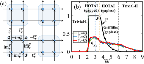
describe the inter-cell hopping along $x$ and $y$, respectively [also see Fig. 1(a) for the hopping parameters]. The system parameters $m_{{\bf r}}^{x}$, $\bar{m}_{{\bf r}}^{x}$, $m_{{\bf r}}^{y}$, $\bar{m}_{{\bf r}}^{y}$, $t_{{\bf r}}^{x}$, $\bar{t}_{{\bf r}}^{x}$, $t_{{\bf r}}^{y}$ and $\bar{t}_{{\bf r}}^{y}$ all take real values. For simplicity without loss of generality, we take the inter-cell hopping magnitude as energy units so that $t_{\bf r}^{x}=\bar{t}_{\bf r}^{x}=t_{\bf r}^{y}=\bar{t}_{\bf r}^{y}=1$. In this case, $h_{x}=\sigma_{-}\otimes\sigma_{z}$ and $h_{y}=\sigma_{0}\otimes\sigma_{-}$ with $\sigma_{-}=[0\,0;1\,0]$ and $\sigma_{0}$ being a $2\times 2$ identity matrix. For a clean system with $m_{\bf r}^{x}=\bar{m}_{\bf r}^{x}=m_{\bf r}^{y}=\bar{m}_{\bf r}^{y}=m$, the system respects a generalized $C_{4}$ symmetry as detailed in Appendix A.

To show that the Hamiltonian (1) describes a higher-order phase supporting zero-energy corner modes in the clean case with $m_{\bf r}^{x}=\bar{m}_{\bf r}^{x}=m_{x}$ and $m_{\bf r}^{y}=\bar{m}_{\bf r}^{y}=m_{y}$, we write the Hamiltonian in momentum space as

Here

where $H_{\nu}(k_{\nu},m_{\nu})=\cos k_{\nu}\sigma_{x}+(m_{\nu}+\sin k_{\nu})\sigma_{y}$ $(\nu=x,y)$ with $\sigma_{\nu}$ $(\nu=x,y,z)$ being the Pauli matrices and $\sigma_{0}$ being a $2\times 2$ identity matrix. To see the presence of zero-energy corner modes in the system, we recast the Hamiltonian (5) to a form in continuous real space by replacing $\sin k_{\nu}$ by $-i\partial_{\nu}$ and $\cos k_{\nu}$ by $1+\partial_{\nu}^{2}/2$ ($\nu=x,y$) so that $H_{\nu}(k_{\nu})\rightarrow\bar{H}_{\nu}$. Considering semi-infinite boundaries along $x$ and $y$, if $|u_{x}\rangle$ and $|u_{y}\rangle$ are zero-energy edge modes of $\bar{H}_{x}$ and $\bar{H}_{y}$, respectively, $|u_{x}\rangle\otimes|u_{y}\rangle$ is a zero-energy mode of $\bar{H}_{0}$ localized at a corner.

Since the system contains only the nearest-neighbor hopping, it respects chiral symmetry, i.e., ${\Pi}H{\Pi}^{-1}=-H$, where $H$ is the first-quantization Hamiltonian and ${\Pi}$ is a unitary matrix. But this system breaks the time-reversal symmetry and thus the particle-hole symmetry, because $h_{0}$ is complex. In contrast, if we generalize the Benalcazar-Bernevig-Hughes (BBH) model Taylor2017Science to the disordered case, it still respects the time-reversal, particle-hole and chiral symmetries. However, these two models are connected through a local transformation and thus have similar topological and localization properties as proved in Appendix B. The equivalence also tells us that our system supports zero-energy corner modes and has quantized quadrupole moments Cho2018arXiv ; Wheeler2018arXiv protected by reflection symmetries. But with disorder breaking the reflection symmetry, one may wonder whether the quadrupole moment is still quantized. Here we prove the quantization of the quadrupole moment maintained by chiral symmetry (see Appendix C), indicating that chiral symmetry can protect a quadrupole topological insulator. We remark that in three dimensions (3D) chiral symmetry maintains the quantization of the octupole moment as proved in Appendix C, indicating that chiral symmetry can protect the third-order topological insulator with zero-energy corner modes in 3D.

To study the disorder effects, we consider the disorder in the intra-cell hopping, that is, $m_{\bf r}^{\nu}=m_{\nu}+W^{\nu}V_{\bf r}^{\nu}$ and $\bar{m}_{\bf r}^{\nu}={m}_{\nu}+\bar{W}^{\nu}\bar{V}_{\bf r}^{\nu}$ with $\nu=x,y$, where ${V}_{\bf r}^{\nu}$ and $\bar{V}_{\bf r}^{\nu}$ are uniformly randomly distributed in $[-0.5,0.5]$ without correlation. Here ${W}^{\nu}$ and $\bar{W}^{\nu}$ represent the disorder strength. For simplicity, we take ${W}^{x}=\bar{W}^{x}={W}^{y}=\bar{W}^{y}=W$. Because of the random character, we perform the average over 200-2000 sample configurations for numerical calculation.

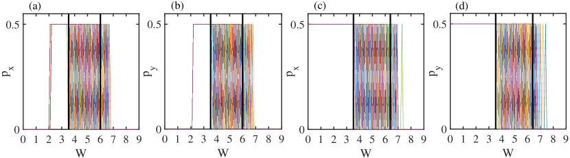
We map out the phase diagram in Fig. 1(b), showing remarkably the presence of a disorder-induced higher-order topological phase transition. To characterize the phase transition, we evaluate the polarization $p_{x}$ ($p_{y}$) of effective boundary Hamiltonians at a $y$-normal ($x$-normal) boundary at half filling. In one dimension, the polarization is equivalent to the Berry phase in a translation invariant system, which can be used as a topological invariant Resta . In fact, the polarization as a topological invariant can be evaluated in real space for a system without translational symmetries based on Resta’s formula Resta ; Prodan2014PRL . For the quadrupole topological phase, we define a topological invariant based on $p_{x}$ and $p_{y}$ as

When $P=1$, the system is in a higher-order topologically nontrivial phase, and when $P=0$, it is in a trivial phase (see Appendix D for its justification for a clean system).

We now generalize it to the disordered case. Specifically, we evaluate the average polarization of the effective boundary Hamiltonian at the $y$-normal boundary (similarly for $x$-normal one) by $p_{x}=\frac{1}{N_{i}}\sum_{n=1}^{N_{i}}|p_{x,n}|$, where $p_{x,n}=\text{Im}\text{log}\langle\Psi_{n}|e^{2\pi i\hat{x}/L_{x}}|\Psi_{n}\rangle/(2\pi)$ Resta with $\hat{x}=\sum_{x}x\hat{n}_{x}$, $\hat{n}_{x}$ being the particle number operator at the site $x$, and $L_{x}$ being the length of the system along $x$ (we also deduct the atomic positive charge contribution). Here $|\Psi_{n}\rangle$ is the ground state at half filling of the boundary Hamiltonian $H_{n}=-G_{2n}(E=0)^{-1}$ with $G_{2n}$ being the $2n$th boundary Green’s function obtained by Dai2008PRB ; Oppen2017PRB

where $h_{n}$ is the Hamiltonian for the $n$th layer and $V_{n-1}$ is the coupling between the $(n-1)$th and $n$th layer. We note that $p_{x,n}$ is quantized to be either $0$ or $0.5$ for each iteration since $H_{n}$ also preserves chiral symmetry. The polarization is evaluated at even steps of Green’s function given that there are two different layers in the clean limit. In the disordered case, the intra-cell hopping parts in $h_{n}$ and $V_{n}$ are randomly generated for each iteration (see Appendix D). The topological invariant $P$ is finally determined.

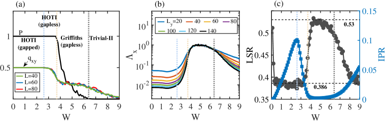
In Fig. 1(b), we plot the topological invariant $P$ as the disorder magnitude increases. We see that $P$ suddenly jumps to $1$ when $W\approx 2.1$, indicating the occurrence of a topological phase transition. $P$ remains quantized to be $1$ until $W>3.5$, where it begins decreasing continuously. This regime corresponds to the Griffiths phase where topologically trivial and nontrivial sample configurations coexist (see Appendix E). When $W>6$, $P$ vanishes, showing that the system reenters into a trivial phase.

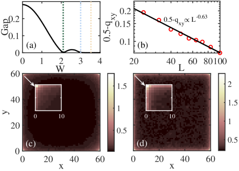
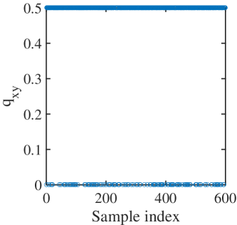
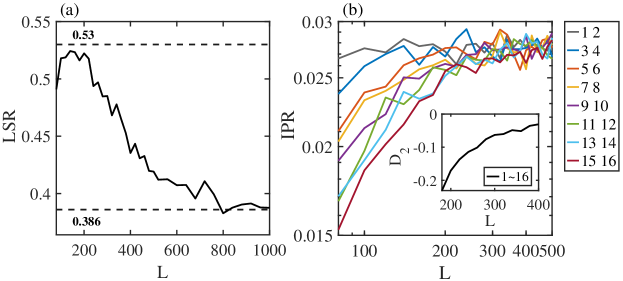
To further identify that the induced topological phase is a quadrupole topological phase, we calculate the quadrupole moment, which can be used as a topological invariant since its quantization is protected by chiral symmetry (see Appendix C). Figure 1(b) shows that the quadrupole moment qualitatively agrees with the results of $P$. Yet, conspicuous discrepancy can be observed. The quadrupole moment $q_{xy}$ over many samples is not quantized to $0.5$ in the regime where $P=1$ [$q_{xy}=0.5$ for most disorder configurations and $q_{xy}=0$ for other configurations (see Fig. C1 in Appendix C)] and the Griffiths regime is much larger. We attribute this to the finite-size effects, given that for the quadrupole moment, we can only perform a computation for a system with its size up to $80$, while to determine $P$, we consider a system with its size up to $500$ and iterations up to $10^{3}$. To be more quantitative, we plot $0.5-q_{xy}$ as the system size $L$ increases when $W=2.6$ in Fig. 2(b), showing a power law decay and thus suggesting that $q_{xy}$ approaches $0.5$ in the thermodynamic limit.

The higher-order topological phase transition occurs as the bulk energy gap closes at $W\approx 2.1$ and reopens, as shown in Fig. 2(a). In fact, the transition is associated with the divergence of the localization length at $W\approx 2.1$ [see Fig. 3(a)]. When $W$ is further increased, the energy gap closes again and remains closed due to the strong disorder scattering, leading to the gapless HOTAI. Even in the gapless regime, the topological invariant $P$ can still be quantized as shown in Fig. 1(b). In fact, in this phase, all the states are localized corresponding to an Anderson insulator (see the following discussion).

To further confirm that the TAI is a higher-order topological state, in Fig. 2(c-d), we display the local density of states (LDOS) at $E=0$ for two typical values of $W$ corresponding to a gapped and gapless topological phase, respectively, clearly showing the presence of zero-energy states localized at corners. The evidence above definitely suggests the existence of HOTAIs.

We now study the localization properties of energy bands in different phases by evaluating their localization length, adjacent level-spacing ratio (LSR), inverse participation ratio (IPR) and fractal dimensions. The LSR is defined as

where $\delta_{i}=E_{i}-E_{i-1}$ with $E_{i}$ being the $i$th eigenenergy sorted in an ascending order and $\sum_{i}$ denotes the sum over an energy bin around the energy $E$ with $N_{E}$ energy levels counted. For localized states, $r\approx 0.386$ corresponding to the Poisson statistics and for extended states of symmetric real Hamiltonians, $r\approx 0.53$ corresponding to the Gaussian orthogonal ensemble (GOE) Huse2007PRB .

The localization property can also be characterized by the real space IPR defined as

This quantity evaluates how much a state in an energy bin around energy $E$ is spatially localized. For an extended state in 2D, $I\propto 1/L^{2}$ with $L$ being the size of a system, which goes zero in the thermodynamic limit; for a state localized in a single unit cell, it is one. It is well known that at the critical point between localized and delocalized phases, the state exhibits multifractal behavior with fractal dimensions $D_{2}$ defined through $I\propto 1/L^{D_{2}}$ Castellani1986 . Clearly, $D_{2}=2$ and $D_{2}=0$ indicates that a state is extended and localized, respectively, in the thermodynamic limit; intermediate values of $D_{2}$ suggests the multifractal state.

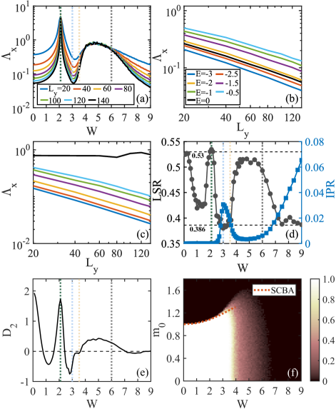
In Fig. 3(a), we plot the normalized localization length $\Lambda_{x}=\lambda_{x}/L_{y}$ (similarly for $\lambda_{y}/L_{x}$) with respect to the disorder strength $W$ at $E=0$ for distinct $L_{y}$, where $\lambda_{\nu}$ ($\nu=x,y$) is the localization length along $\nu$ calculated by the transfer matrix method Kramer1983 . In the gapless HOTAI and trivial-II phases, we see the decrease of $\Lambda_{x}$ as $L_{y}$ is increased, suggesting that the states at $E=0$ are localized. The decline can also be clearly seen in Fig. 3(b) where $\Lambda_{x}$ versus $L_{y}$ is plotted for $W=3.2$ for distinct energies. In fact, all states are localized in these two phases as detailed in the following discussion. This shows that even in the higher-order case, the topology can be carried by localized bulk states. Being localized for the states in these regimes is also evidenced by their relatively large IPR and the LSR approaching $0.386$ [see Fig. 3(d)]. In these regimes, the fractal dimension $D_{2}$ becomes negative or approaches zero [see Fig. 3(e)], further indicating that the states around zero energy are localized. We note that the negative $D_{2}$ arises from finite-size effects. It indicates that the IPR rises with increasing the system size, suggesting that the states are localized (see Appendix F for the finite-size analysis).

Figure 3(a) also demonstrates the existence of a regime (corresponding to the Griffiths regime) where $\Lambda_{x}$ at $E=0$ remains almost unchanged as $L_{y}$ increases, suggesting a multifractal phase in this regime. The multifractal phase resides between two localized phases, which is very different from the conventional wisdom that a multifractal phase lives at the critical point between delocalized and localized phases. In fact, only the states at or very near $E=0$ become multifractal, and all other states remain localized [see Fig. 3(c)]. The multifractal properties are also evidenced by the fractal dimension of the states around zero energy as shown in Fig. 3(e).

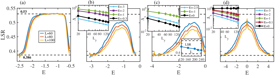
In the gapped regime, there are trivial-I and gapped HOTAI phases. In the trivial phase, the states at the band edge around zero energy exhibit the LSR close to $0.386$ [see Fig. 3(d)], suggesting the localized property of these states. The localized property is also evidenced by the negative $D_{2}$ (in the region around $W=1$) [see Fig. 3(e)]. We note that near the phase transition points of $W=0$ and $W=2.1$, the states exhibit delocalized properties due to the large localization length. In the gapped HOTAI, Fig. 3(d) and (e) illustrate that the LSR experiences a drop from around $0.53$ to $0.386$ and $D_{2}$ drops from $1.72$ to negative values, suggesting that the states at the band edge undergo a phase transition from delocalized to localized ones.

The above results indicate that for strong disorder, all states are localized in the gapless HOTAI and the trivial-II phase. Yet in the Griffiths phase, all states are localized except at $E=0$ where the states become multifractal. For weak disorder, all states can be localized in the topological regime. In the trivial-I phase, the states at the band edge around zero energy are localized.

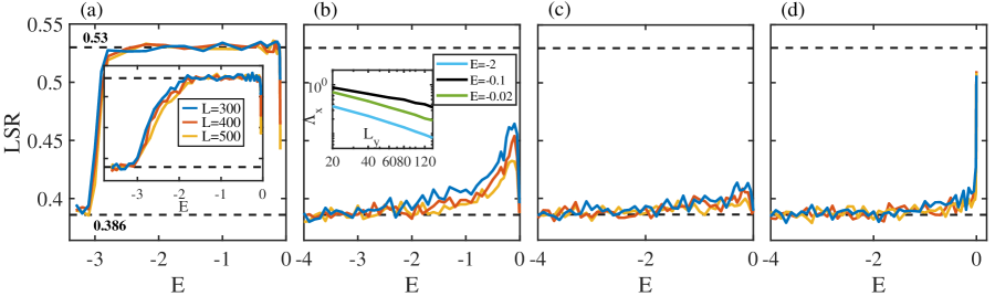
In the following, we provide more evidence on localization properties. Figure 4 shows the LSR as a function of energy for five different disorder amplitudes. For small $W$ corresponding to the trivial-I phase [Fig. 4(a) and its inset], the LSR remains around $0.53$ except at the lower band edge where it exhibits a sudden drop towards $0.386$, indicating that the states at the band edge are localized. But we cannot claim the existence of mobility edges in the trivial-I phase given that it is very possible that the delocalized behavior is caused by the finite-size effects, which is very difficult to identify since the localization length is huge for the weak disorder. In the gapped HOTAI, while we cannot conclusively determine that all states are localized when $W$ is near the transition point, we show that this occurs when $W$ is larger. For instance, when $W=2.8$, Fig. 4(b) illustrates that the LSR decreases towards $0.386$ with the increase of the system size. We also plot the normalized localization length with respect to $L_{y}$ for different energies, the fall of which clearly suggests that the states are localized. These indicators show that all the states are localized. Similarly, Fig. 4(c) indicates that all the states are localized in the gapless HOTAI phase. But in the Griffiths regime, all the states are localized except at $E=0$ where the LSR remains unchanged as the system size is increased [see Fig. 4(d)].

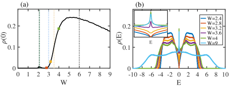
We also compute the density of states (DOS) at $E=0$ with respect to the disorder strength $W$ as shown in Fig. 5(a). The DOS is defined as $\rho(E)=\sum_{\bf r}\rho(E,{\bf r})/(4L_{x}L_{y})$, which is normalized to one, i.e., $\int dE\rho(E)=1$. Here $\rho(E,{\bf r})=[\sum_{j}\delta(E-E_{j})\sum_{\nu=1}^{4}|\Psi_{E_{j},{\bf r}\nu}|^{2}]$ describes the LDOS, where $\Psi_{E_{i},{\bf r}\nu}$ denotes the spatial eigenstate of the system with periodic boundaries corresponding to the eigenenergy $E_{i}$, and $[\cdots]$ denotes the average over different samples. The DOS rises to the maximum in the multifractal phase and then fall in the trivial-II phase. Specifically, we see the development of a very narrow peak of the DOS at $E=0$ in this regime [Fig. 5(b)].

We now explain the disorder induced quadrupole topological insulator based on the self-consistent Born approximation (SCBA) Beenakker2009PRL . As introduced in Sec. II, we consider a disordered system by adding the following random intra-cell hopping terms at each unit cell ${\bf r}$

where $V_{1}^{\prime}=(V_{1}+V_{2})/2$, $V_{2}^{\prime}=(V_{1}-V_{2})/2$, $V_{3}^{\prime}=(V_{3}+V_{4})/2$, $V_{4}^{\prime}=(V_{3}-V_{4})/2$, and $U_{1}=\sigma_{y}\otimes\sigma_{z}$, $U_{2}=\sigma_{y}\otimes\sigma_{0}$, $U_{3}=\sigma_{0}\otimes\sigma_{y}$, $U_{4}=\sigma_{z}\otimes\sigma_{y}$. Here we have changed the notation in Sec. II by $V^{x}\rightarrow V_{1}$, $\bar{V}^{x}\rightarrow V_{2}$, $V^{y}\rightarrow V_{3}$ and $\bar{V}^{y}\rightarrow V_{4}$ for convenience. Since we are interested in disorder without correlations, we require

for $i,j=1,2,3,4$ with $\langle\cdots\rangle$ denoting the average over disorder ensembles.

Based on the self-consistent Born approximation, the effective Hamiltonian at $E=0$ is given by $H_{\textrm{eff}}({\bf k})=H_{0}({\bf k})+\Sigma(E=0)$ where the self-energy $\Sigma$ in the presence of disorder can be calculated through the following self-consistent equation

where $G=[(E+i0^{+})I-H_{0}({\bf k})-\Sigma(E)]^{-1}$. At energy $E=0$, we find numerically that the self-energy can be expanded as

with $\Sigma_{0},\Sigma_{x},\Sigma_{y}$ being real numbers. It is clear to see that the topological masses $m_{x}$ and $m_{y}$ associated with topological properties are renormalized by disorder to new values

Based on Eq. (13), we first approximate the self-energy $\Sigma$ by taking $\Sigma=0$ in the right-hand side of the equation, yielding

where

with $\nu=x,y$. When $m_{x}>1$ and $m_{y}>1$, both $\Sigma_{x}$ and $\Sigma_{y}$ are negative due to the positive integrands, leading to a topological phase transition when the disorder strength $W$ is sufficiently large so that $m_{x}^{\prime}<1$ and $m_{y}^{\prime}<1$. We also numerically solve the Eq. (13) self-consistently to determine $\Sigma_{x}$ and $\Sigma_{y}$ and plot the results in Fig. 3(f). For weak disorder, the results agree very well with the numerical phase boundary.

In this section, we study the effects of disorder on HOTIs. Specifically, we consider $m_{x}=m_{y}=0.5$ corresponding to a HOTI in the clean limit. We find that the topological phase is stable against weak disorder as evidenced by the quantized topological invariant $P$ in Fig. 6(a). When the disorder strength becomes sufficiently strong, it enters into a Griffiths regime with fractional $P$ and finally becomes a trivial phase. The strong disorder also closes the energy gap when $W>2.6$. In the gapless HOTI and trivial-II phases, all states are localized, as evidenced by the normalized localization length, LSR and IPR [see Fig. 6(b) and (c)]. In the Griffiths regime, the states at $E=0$ are multifractal and all other states are localized [see Fig. 6(b)]. In the disordered gapped HOTI, we find that for weak disorder, the states near the band edge are localized as shown by the LSR around $0.386$ in Fig. 6(c). For larger disorder, all the states become localized in this phase.

Figure 7 further plots the LSR with respect to $E$ for four different disorder strength. When the disorder is weak, e.g., $W=1$, the LSR shows that the states near the band edge are localized in the gapped HOTI [Fig. 7(a)]. Yet, when $W=2$, the LSR of all the states decreases towards $0.386$ with the increase of the system size, reflecting that all the states are localized. The localized property is also signalled by the decline of the normalized localization length with increasing $L_{y}$ [Fig. 7(b)]. Similarly, in the gapless HOTI, all the states are localized as shown in Fig. 7(c). In this case, the LSR at $E=-1$ decreases towards $0.386$ as the system size is increased, providing further evidence for localization. In the Griffiths regime, the LSR becomes smaller for larger system sizes except at $E=0$ where it remains unchanged, suggesting that the states at $E=0$ are multifractal and all other states are localized. The multifractal property is also reflected by the unchanged property of the normalized localization length as $L_{y}$ is increased [Fig. 7(d)].

The BBH model has been experimentally realized in several metamaterials, such as microwave, phononic, photonic and topolectrical circuit systems Huber2018Nature ; Bahl2018Nature ; Thomale2018NP ; Hafezi2019NP . In fact, some systems, such as silicon ring resonators Hafezi2019NP , have demonstrated the robustness of zero-energy corner modes to certain disorders. The HOTAI can be easily realized in these systems when the off-diagonal hopping disorder is considered in the experimentally realized BBH model. The BBH model has also been implemented in topolectrical circuits, and zero-energy corner modes are probed by measuring two-point impedances Thomale2018NP . One can involve disorder in the system by tuning the capacitance of capacitors and inductance of inductors to realize the HOTAI, as we have proved that this model is equivalent to our model in topological and localization properties (see Appendix B). In the following, we discuss in detail an experimental scheme to realize the Hamiltonian (1) using topolectrical circuits and show that the HOTAI phase can be detected by two-point impedance measurements.

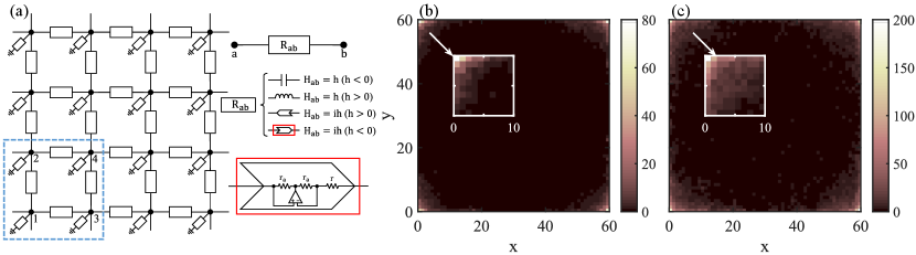
Let us consider an electric network composed of different nodes and electric element connecting nodes, as shown in Fig. 8(a). We denote the input current and voltage of each node $a$ by $I_{a}$ and $V_{a}$, respectively. According to Kirchhoff’s law, the circuit at a frequency of $\omega$ should satisfy the relation

where $R_{ab}$ is the admittance of the corresponding electric element between the node $a$ and $b$, and $R_{a}$ is the admittance of the electric element between the node $a$ and the ground. We can rewrite the above equation into a compact form as

where ${\bf I}$ and ${\bf V}$ are $N$-component column vectors with components $I_{a}$ and $V_{a}$ for $N$ nodes, respectively. Here the matrix $J$ is the circuit Laplacian. Then we can simulate our Hamiltonian $H$ with the Laplacian $J(\omega)$ at a proper frequency $\omega$ through

Each node in the circuit represents one lattice site in our Hamiltonian, and each electric element linking two nodes represents the corresponding hopping between the sites, which can be either a capacitor, or an inductor, or a negative impedance converter with current inversion (INIC). For two nodes in the circuit, the electric element between them is determined according to the corresponding matrix element $H_{ab}$ between the site $a$ and $b$ in our Hamiltonian, as illustrated in Fig. 8(a). Specifically, for two neighboring sites in our Hamiltonian, if $H_{ab}$ is a positive (negative) real number, the electric element between $a$ and $b$ should be an inductor (a capacitor) with inductance (capacitance) $\frac{1}{\omega H_{ab}}$ ($-\frac{H_{ab}}{\omega}$). For the case that $H_{ab}$ is an imaginary number, we should connect the two nodes using an INIC with resistance $\frac{1}{|H_{ab}|}$ and proper direction. In addition, we connect every node with the ground by appropriate electric elements to eliminate the extra diagonal terms in the Laplacian.

Similar to the experimental work Thomale2018NP , we utilize the two-point impedance measurement in the circuit to characterize the zero-energy corner modes in the HOTAI phase. The two-point impedance between node $a$ and $b$ is defined as

where $\psi_{n,a}$ is the component for the node $a$ of the $n$th eigenvector of $J$ with eigenvalue $j_{n}$. We define the impedance of each unit cell $Z(x,y)$ as the average two-point impedance between nearest-neighbor nodes within each unit cell as

where $Z_{ij}(x,y)$ denotes the two-point impedance between the $i$th node and $j$th node of the unit cell $(x,y)$. Fig. 8(b) and (c) plot the magnitude of $Z(x,y)$ averaged over $400$ random samples under open boundary conditions for two values of $W$ within HOTAI regime for $m_{x}=m_{y}=1.1$, which clearly show the impedance resonance near the corners corresponding to the presence of zero-energy corner modes of the Hamiltonian.

In summary, we have discovered the HOTAI in a 2D disordered system with chiral symmetry. Specifically, we show that a topologically trivial phase can transition into a quadrupole topological phase, when disorder is added. We find gapped and gapless HOTAIs and a Griffiths regime. In the gapless HOTAI, all the states are localized, while in the Griffiths regime, the states at zero energy are multifractal and other states are localized. The Griffiths regime corresponds to a critical regime between two localized phases: a gapless HOTAI and a trivial phase. We also propose an experimental scheme with topolectrical circuits to realize the HOTAI. Our results demonstrate that disorder can induce quadrupole topological insulators with peculiar localization properties from a trivial phase and thus opens a new avenue for studying the role of disorder in higher-order topological phases.

Note added: Recently, we became aware of two related work Shen2020PRL ; Zhang2020arXiv .

In the clean case, when $m_{x}=m_{y}$ and $t_{x}=t_{y}$, the Hamiltonian (1) in the main text respects a generalized $C_{4}$ symmetry,

where

with

and $g$ being a $C_{4}$ rotation operator such that $g{\bf r}=(-y,x)$.

In momentum space, let us write $\hat{H}=\sum_{\bf k}\hat{c}_{\bf k}^{\dagger}H({\bf k})\hat{c}_{\bf k}$ with $\hat{c}_{\bf k}^{\dagger}=(\begin{array}[]{cccc}\hat{c}_{{\bf k}1}^{\dagger}&\hat{c}_{{\bf k}2}^{\dagger}&\hat{c}_{{\bf k}3}^{\dagger}&\hat{c}_{{\bf k}4}^{\dagger}\end{array})$. The generalized $C_{4}$ symmetry takes the following form

where ${\bf k}^{\prime}=(k_{x},k_{y}-\pi)$ and

In this Appendix, we will prove that our model is equivalent to the BBH model in topological and localization properties. The BBH model reads

where $\tilde{h}_{0}$ is a real matrix expressed as

This model respects the time-reversal, particle-hole and chiral symmetries.

While the two Hamiltonians have different symmetries, they are closely related by a local transformation $U_{{\bf r}}=\text{diag}(i^{x+y-1},i^{x+y},i^{x+y},i^{x+y+1})$, that is, $U_{{\bf r}}^{\dagger}h_{0}U_{{\bf r}}=\tilde{h}_{0}$, $U_{{\bf r}}^{\dagger}h_{x}U_{{\bf r}+{\bf e}_{x}}={h}_{x}$ and $U_{{\bf r}}^{\dagger}h_{y}U_{{\bf r}+{\bf e}_{y}}={h}_{y}$. Specifically, one can transform $\hat{H}$ in Eq. (1) to $\hat{\tilde{H}}$ by the transformation $\hat{c}_{{\bf r}}\rightarrow U_{{\bf r}}\hat{c}_{{\bf r}}$. In other words, if $\Psi_{E_{i},{\bf r}\nu}$ is a spatial eigenstate of $H$, then $\tilde{\Psi}_{E_{i},{\bf r}\nu}=(-i)^{f_{{\bf r}\nu}}\Psi_{E_{i},{\bf r}\nu}$ with $f_{{\bf r}1}=x+y-1$, $f_{{\bf r}2}=f_{{\bf r}3}=x+y$, and $f_{{\bf r}4}=x+y+1$ is an eigenstate of $\tilde{H}$ corresponding to the same energy $E_{i}$. Here $H$ and $\tilde{H}$ are the first-quantization Hamiltonians of $\hat{H}$ and $\hat{\tilde{H}}$, respectively. Therefore, $\hat{H}$ and $\hat{\tilde{H}}$ have the same energy spectrum and density profiles, indicating identical localization properties that they possess. In addition, this local phase transformation does not change the topological property, and thus the two Hamiltonians have the same topology. Under open boundary conditions, the two models are connected by the transformation irrelevant of the system size. Yet, under periodic boundary conditions, the transformation works well only when $L_{x}$ and $L_{y}$ are integer multiples of four. For topological property, the two models should be equivalent irrelevant of a system size given that the topology does not depend on a specific system size. For localization property, we have also calculated the IPR and LSR of the two Hamiltonians with their sizes being odd and find similar results, showing that their localization properties are irrelevant of the parity of a system size.

In this Appendix, we will prove that the quadrupole moment is protected to be quantized by chiral symmetry and thus can be used as a topological invariant. Note that the quadrupole moment may not characterize the physical quadrupole moment, we here are only interested in the formula as a topological invariant. We consider the quadrupole moment defined by Wheeler2018arXiv ; Cho2018arXiv

where $\hat{Q}_{xy}=\sum_{j=1}^{n_{c}}\hat{x}_{j}\hat{y}_{j}/(L_{x}L_{y})$ with $\hat{x}_{j}$ ($\hat{y}_{j}$) denoting the $x$-position ($y$-position) operator for electron $j$ with $n_{c}=2L_{x}L_{y}$ (the number of occupied states in our model) at half filling, and $|\Psi_{G}\rangle$ is the many-body ground state of electrons in the system. Here $\tilde{q}_{xy}=\frac{1}{2\pi}\mathrm{Im}[\log\langle\Psi_{G}|e^{2\pi i\hat{Q}_{xy}}|\Psi_{G}\rangle]$ is the contribution from occupied electrons, and $q_{xy}^{(0)}=\frac{1}{2}\sum_{j=1}^{n_{a}}x_{j}y_{j}/(L_{x}L_{y})$ is the contribution from the background positive charge distribution where $(x_{j},y_{j})$ denotes the position of the $j$th atomic orbital. Here, $n_{a}$ is the total number of atomic orbitals so that the single-particle Hamiltonian is a $n_{a}\times n_{a}$ matrix. At half filling, $n_{a}=2n_{c}$.

Let us write the many-body wave function of occupied electrons in real space representation as

where $\psi_{n}$ represents the $n$th occupied eigenstate of a first-quantization Hamiltonian. Then, the quadrupole moment of occupied electrons $\tilde{q}_{xy}$ can be evaluated through

where

$\tilde{\psi}_{n}({\bf r}\nu)=e^{i2\pi xy/(L_{x}L_{y})}\psi_{n}({\bf r}\nu)$ and $\langle\psi_{m}|\tilde{\psi}_{n}\rangle=\sum_{{\bf r}\alpha}\psi_{m}^{*}({\bf r}\alpha)\tilde{\psi}_{n}({\bf r}\alpha)$. Let us define $U_{o}=\left(|\psi_{1}\rangle,|\psi_{2}\rangle,\cdots,|\psi_{n_{c}}\rangle\right)$ which is a $n_{a}\times n_{c}$ matrix representing the occupied states of electrons. Then we can express the quadrupole moment of occupied electrons as

where we define a $n_{a}\times n_{a}$ diagonal matrix $\hat{D}=\text{diag}\{e^{2\pi ix_{j}y_{j}/(L_{x}L_{y})}\}_{j=1}^{n_{a}}$ with $(x_{j},y_{j})$ denoting the position of $j$-th atomic orbital.

For a generic Hamiltonian in real space $H$ with chiral (sublattice) symmetry, ${\Pi}H{\Pi}^{-1}=-H$, if $|\psi_{n}\rangle$ is an eigenstate of $H$ corresponding to energy $E_{n}$, ${\Pi}|\psi_{n}\rangle$ is also an eigenstate of $H$ with energy $-E_{n}$, corresponding to an unoccupied state. The set $\{{\Pi}|\psi_{1}\rangle,{\Pi}|\psi_{2}\rangle,\cdots,{\Pi}|\psi_{n_{c}}\rangle\}$ therefore constitutes the unoccupied states. We then define $U_{u}=\left({\Pi}|\psi_{1}\rangle,{\Pi}|\psi_{2}\rangle,\cdots,{\Pi}|\psi_{n_{c}}\rangle\right)={\Pi}U_{o}$ representing the unoccupied states of electrons. The quadrupole moment $\tilde{q}_{xy}^{u}$ for the unoccupied states is

Clearly, $\hat{D}$ commutes with the chiral (sublattice) symmetry transformation $\Pi$, i.e., $\left[\hat{D},\Pi\right]=0$,

Let us define $q_{xy}^{u}\equiv\left[\tilde{q}_{xy}^{u}-q_{xy}^{(0)}\right]\mod 1$. Then we will have

Next we will prove that $q_{xy}+q_{xy}^{u}=0\mod 1$, i.e., $\tilde{q}_{xy}+\tilde{q}_{xy}^{u}-2q_{xy}^{(0)}=0\mod 1$.

References

- (1) W. A. Benalcazar, B. A. Bernevig, and T. L. Hughes, Quantized electric multipole insulators, Science 357, 61 (2017).
- (2) M. Sitte, A. Rosch, E. Altman, and L. Fritz, Topological Insulators in Magnetic Fields: Quantum Hall Effect and Edge Channels with a Nonquantized Term, Phys. Rev. Lett. 108, 126807 (2012).
- (3) F. Zhang, C. L. Kane, and E. J. Mele, Surface State Magnetization and Chiral Edge States on Topological Insulators, Phys. Rev. Lett. 110, 046404 (2013).
- (4) R.-J. Slager, L. Rademaker, J. Zaanen, and L. Balents, Impurity-bound states and Green’s function zeros as local signatures of topology, Phys. Rev. B 92, 085126 (2015).
- (5) Z. Song, Z. Fang, and C. Fang, -Dimensional Edge States of Rotation Symmetry Protected Topological States, Phys. Rev. Lett. 119, 246402 (2017).
- (6) J. Langbehn, Y. Peng, L. Trifunovic, F. von Oppen, and P. W. Brouwer, Reflection-Symmetric Second-Order Topological Insulators and Superconductors, Phys. Rev. Lett. 119, 246401 (2017).
- (7) F. Schindler, A. M. Cook, M. G. Vergniory, Z. Wang, S. S. P. Parkin, B. A. Bernevig, and T. Neupert, Higher-order topological insulators, Sci. Adv. 4, eaat0346 (2018).
- (8) L. Trifunovic and P. W. Brouwer, Higher-order bulk-boundary correspondence for topological crystalline phases, Phys. Rev. X 9, 011012 (2019).
- (9) D. Călugăru, V. Juričić, and B. Roy, Higher-order topological phases: A general principle of construction, Phys. Rev. B 99, 041301(R) (2019).
- (10) X.-L. Sheng, C. Chen, H. Liu, Z. Chen, Z.-M. Yu, Y. X. Zhao, and S. A. Yang, Two-Dimensional Second-Order Topological Insulator in Graphdiyne, Phys. Rev. Lett. 123, 256402 (2019).
- (11) B. Huang and W. V. Liu, Floquet Higher-Order Topological Insulators with Anomalous Dynamical Polarization, Phys. Rev. Lett. 124, 216601 (2020).
- (12) H. Hu, B. Huang, E. Zhao, and W. V. Liu, Dynamical Singularities of Floquet Higher-Order Topological Insulators, Phys. Rev. Lett. 124, 057001 (2020).
- (13) Y.-B. Yang, K. Li, L.-M. Duan, and Y. Xu, Type-II quadrupole topological insulators, Phys. Rev. Res. 2, 033029 (2020).
- (14) A. Tiwari, M.-H. Li, B. A. Bernevig, T. Neupert, and S. A. Parameswaran, Unhinging the Surfaces of Higher-Order Topological Insulators and Superconductors, Phys. Rev. Lett. 124, 046801 (2020).
- (15) H. Araki, T. Mizoguchi, and Y. Hatsugai, Phase diagram of a disordered higher-order topological insulator: A machine learning study, Phys. Rev. B 99, 085406 (2019).
- (16) Z. Su, Y. Kang, B. Zhang, Z. Zhang, and H. Jiang, Disorder induced phase transition in magnetic higher-order topological insulator: A machine learning study, Chin. Phys. B 28, 117301 (2019).
- (17) S. Franca, D. V. Efremov, and I. C. Fulga, Phase-tunable second-order topological superconductor, Phys. Rev. B 100, 075415 (2019).
- (18) C.-A. Li and S.-S. Wu, Topological states in generalized electric quadrupole insulators, Phys. Rev. B 101, 195309 (2020).
- (19) A. Agarwala, V. Juričić, and B. Roy, Higher-order topological insulators in amorphous solids, Phys. Rev. Res. 2, 012067(R) (2020).
- (20) C. Wang and X. R. Wang, Disorder-induced quantum phase transitions in three-dimensional second-order topological insulators, Phys. Rev. Res. 2, 033521 (2020).
- (21) F. Evers and A. D. Mirlin, Anderson transitions, Rev. Mod. Phys. 80, 1355 (2008).
- (22) J. Li, R.-L. Chu, J. K. Jain, and S.-Q. Shen, Topological Anderson Insulator, Phys. Rev. Lett. 102, 136806 (2009).
- (23) C. W. Groth, M. Wimmer, A. R. Akhmerov, J. Tworzydło, and C. W. J. Beenakker, Theory of the Topological Anderson Insulator, Phys. Rev. Lett. 103, 196805 (2009).
- (24) H. Jiang, L. Wang, Q.-F. Sun, and X. C. Xie, Numerical study of the topological Anderson insulator in HgTe/CdTe quantum wells, Phys. Rev. B 80, 165316 (2009).
- (25) H.-M. Guo, G. Rosenberg, G. Refael, and M. Franz, Topological Anderson Insulator in Three Dimensions, Phys. Rev. Lett. 105, 216601 (2010).
- (26) A. Altland, D. Bagrets, L. Fritz, A. Kamenev, and H. Schmiedt, Quantum Criticality of Quasi-One-Dimensional Topological Anderson Insulators, Phys. Rev. Lett. 112, 206602 (2014).
- (27) I. Mondragon-Shem, T. L. Hughes, J. Song, and E. Prodan, Topological Criticality in the Chiral-Symmetric AIII Class at Strong Disorder, Phys. Rev. Lett. 113, 046802 (2014).
- (28) P. Titum, N. H. Lindner, M. C. Rechtsman, and G. Refael, Disorder-Induced Floquet Topological Insulators, Phys. Rev. Lett. 114, 056801 (2015).
- (29) C. Liu, W. Gao, B. Yang, and S. Zhang, Disorder-Induced Topological State Transition in Photonic Metamaterials, Phys. Rev. Lett. 119, 183901 (2017).
- (30) C.-Z. Chen, J. Song, H. Jiang, Q.-F. Sun, Z. Wang, and X. C. Xie, Disorder and Metal-Insulator Transitions in Weyl Semimetals, Phys. Rev. Lett. 115, 246603 (2015).
- (31) S. Stützer, Y. Plotnik, Y. Lumer, P. Titum, N. H. Lindner, M. Segev, M. C. Rechtsman, and A. Szameit, Photonic topological Anderson insulators, Nature (London) 560, 461 (2018).
- (32) E. J. Meier, F. A. An, A. Dauphin, M. Maffei, P. Massignan, T. L. Hughes, and B. Gadway, Observation of the topological Anderson insulator in disordered atomic wires, Science 362, 929 (2018).
- (33) A. Altland and M. R. Zirnbauer, Nonstandard symmetry classes in mesoscopic normal-superconducting hybrid structures, Phys. Rev. B 55, 1142 (1997).
- (34) C. W. J. Beenakker, Random-matrix theory of quantum transport, Rev. Mod. Phys. 69, 731 (1997).
- (35) F. Haake, Quantum Signatures of Chaos (Springer-Verlag, Berlin, Heidelberg, 2006).
- (36) S. Ryu, A. P. Schnyder, A. Furusaki, and A. W. W. Ludwig, Topological insulators and superconductors: tenfold way and dimensional hierarchy, New J. Phys. 12, 065010 (2010).
- (37) F. J. Dyson, The Dynamics of a Disordered Linear Chain, Phys. Rev. 92, 1331 (1953).
- (38) G. Theodorou and M. H. Cohen, Extended states in a one-demensional system with off-diagonal disorder, Phys. Rev. B 13, 4597 (1976).
- (39) T. P. Eggarter and R. Riedinger, Singular behavior of tight-binding chains with off-diagonal disorder, Phys. Rev. B 18, 569 (1978).
- (40) A. Eilmes, R. A. Römer, and M. Schreiber, The two-dimensional Anderson model of localization with random hopping, Eur. Phys. J. B 1, 29 (1998).
- (41) P. W. Brouwer, C. Mudry, B. D. Simons, and A. Altland, Delocalization in Coupled One-Dimensional Chains, Phys. Rev. Lett. 81, 862 (1998).
- (42) R. Okugawa, S. Hayashi, and T. Nakanishi, Second-order topological phases protected by chiral symmetry, Phys. Rev. B 100, 235302 (2019).
- (43) Q.-B. Zeng, Y.-B. Yang, and Y. Xu, Higher-order topological insulators and semimetals in generalized Aubry-André-Harper models, Phys. Rev. B 101, 241104(R) (2020).
- (44) B. Kang, K. Shiozaki, and G. Y. Cho, Many-body order parameters for multipoles in solids, Phys. Rev. B 100, 245134 (2019).
- (45) W. A. Wheeler, L. K. Wagner, and T. L. Hughes, Many-body electric multipole operators in extended systems, Phys. Rev. B 100, 245135 (2019).
- (46) R. Resta, Quantum-Mechanical Position Operator in Extended Systems, Phys. Rev. Lett. 80, 1800 (1998).
- (47) X. Dai, T. L. Hughes, X.-L. Qi, Z. Fang, and S.-C. Zhang, Helical edge and surface states in HgTe quantum wells and bulk insulators, Phys. Rev. B 77, 125319 (2008).
- (48) Y. Peng, Y. Bao, and F. von Oppen, Boundary Green functions of topological insulators and superconductors, Phys. Rev. B 95, 235143 (2017).
- (49) V. Oganesyan and D. A. Huse, Localization of interacting fermions at high temperature, Phys. Rev. B 75, 155111 (2007).
- (50) C. Castellani and L. Peliti, Multifractal wavefunction at the localisation threshold, J. Phys. A 19, L429 (1986).
- (51) A. MacKinnon and B. Kramer, The scaling theory of electrons in disordered solids: Additional numerical results, Z. Phys. B 53, 1 (1983).
- (52) M. Serra-Garcia, V. Peri, R. Süsstrunk, O. R. Bilal, T. Larsen, L. G. Villanueva, and S. D. Huber, Observation of a phononic quadrupole topological insulator, Nature (London) 555, 342 (2018).
- (53) C. W. Peterson, W. A. Benalcazar, T. L. Hughes, and G. Bahl, A quantized microwave quadrupole insulator with topologically protected corner states, Nature (London) 555, 346 (2018).
- (54) S. Imhof, C. Berger, F. Bayer, J. Brehm, L. W. Molenkamp, T. Kiessling, F. Schindler, C. H. Lee, M. Greiter, T. Neupert, and R. Thomale, Topolectrical-circuit realization of topological corner modes, Nat. Phys. 14, 925 (2018).
- (55) S. Mittal, V. V. Orre, G. Zhu, M. A. Gorlach, A. Poddubny, and M. Hafezi, Photonic quadrupole topological phases, Nat. Photon. 13, 692 (2019).
- (56) C.-A. Li, B. Fu, Z.-A. Hu, J. Li, and S.-Q. Shen, Topological Phase Transitions in Disordered Electric Quadrupole Insulators, Phys. Rev. Lett. 125, 166801 (2020).
- (57) W. Zhang, D. Zou, Q. Pei, W. He, J. Bao, H. Sun, and X. Zhang, Experimental Observation of Higher-Order Topological Anderson Insulators, arXiv:2008.00423.