Hilbert space representation for quasi-Hermitian position-deformed Heisenberg algebra and Path integral formulation

Thomas Katsekpor^1,a, Latévi M. Lawson^2,3,b, Prince K. Osei^2,c and Ibrahim Nonkané^4,d

¹Department of Mathematics, University of Ghana, Legon, Accra, Ghana

²African Institute for Mathematical Sciences (AIMS) Ghana, Accra, Ghana

³Université de Lomé, Faculté des Sciences, Departement de Physique, Lomé, Togo

⁴Departement d’Économie et de Mathématiques Appliquées,
IUFIC, Université Thomas Sankara, Burkina faso

tkatsekpor@ug.edu.gh^a, Latevi@aims.edu.gh^b, pkosei@aims.edu.gh^c, inonkane@univouaga2.bf ^d

Abstract

Position deformation of a Heisenberg algebra and Hilbert space representation of both maximal length and minimal momentum uncertainties may lead to loss of Hermiticity of some operators that generate this algebra. Consequently, the Hamiltonian operator constructed from these operators are also not Hermitian. In the present paper, with an appropriate positive-definite Dyson map, we establish the hermiticity of these operators by means of a quasi-similarity transformation. We then construct Hilbert space representations associated with these quasi-Hermitian operators that generate a quasi-Hermitian Heisenberg algebra. With the help of these representations we establish the path integral formulation of any systems in this quasi-Hermitian algebra. Finally, using the path integral of a free particle as an example, we demonstrate that the Euclidean propagator, action, and kinetic energy of this system are constrained by the standard classical mechanics limits.

Keywords: Non-Hermitian Hamiltonian, Quasi-Hermitian Hamiltonian, Generalized Uncertainty Principle; Quantum Gravity; Path Integral.

1 Introduction

The study of Hilbert space representation of deformations for the uncertainly relation provides a promising approach to understand quantum gravity at the Planck scale [1, 2, 3, 4, 5, 6, 7, 8, 9, 10, 11, 12]. They consist of quadratic Heisenberg algebra deformations in either momentum or position operators [13, 14, 15, 16, 17, 18, 19]. It is well known that these deformations lead to maximal length and minimal momentum uncertainties and induce among other consequences a loss of hermiticity of some operators that generate this algebra [13]. Consequently, Hamiltonians $\hat{H}$ of systems involving these operators will in general also not be Hermitian. An immediate difficulty that arises when $\hat{H}$ is not Hermitian is that, the time evolution operator $\hat{U}(t)=e^{-\frac{i}{\hbar}\hat{H}}$ is not unitary with respect to the inner product, resulting in non-conservation of the inner product under this time-evolution.

Non-Hermitian Hamiltonians with real spectra in this context has been well studied in the past few decades [20, 21, 22, 23, 24, 25, 26, 27, 28, 29, 30, 31, 32, 33, 34, 35, 36, 37, 38, 39]. The pseudo-Hermiticity and quasi-Hermiticity are two commonly used concepts that are introduced in the literature in order to map these non-Hermitian Hamiltonian operators into their Hermitian counterparts and guarantee the conservation of the Hilbert space structure [20, 26, 27, 31, 32, 33, 38, 40, 41, 42, 43]. Both concepts are closely related and the distinction between them is not always made, see for example [30, 32, 40, 41]. In the pseudo-Hermitian quantum mechanics [22, 27, 32, 33, 38, 40] one constructs the so called pseudo-inner product by which the Hamiltonian (non-Hermitian with respect to the conventional inner product of quantum mechanics) having real spectrum is pseudo-similar to its adjoint via a metric operator, that is., a strictly positive, hermitian and invertible operator. Quasi-H,ermitian quantum mechanics [22, 29, 30, 31, 37, 38, 39, 43, 44] are just the ordinary quantum mechanics with the conventional inner product by which the non-hermitian Hamiltonian is quasi-similar to its adjoint via a Dyson map [21], a unique positive-definite square root of the former metric operator. In this work, we study a the application of both concepts to a particular position deformation of a Heisenberg algebra. Since the concept of quasi-hermitian quantum mechanics and ordinary quantum mechanics are equivalent, we deal with the dynamics of systems within this

A recently proposed quadratic position-deformed Heisenberg algebra in 2D with simultaneously existence of minimal and maximal length uncertainties [45]. It has been shown that this algebra could be a promising candidate to probe quantum gravity [35, 46, 47, 48, 49]. In the current work, we study the one dimensional case of this algebra which exhibits a maximal length and a minimal momentum uncertainties. As has been shown in [45, 46, 48, 49], the deformation induces a loss of hermiticity of the momentum operator which consequently of the corresponding Hamiltonian operator. With an appropriate positive definite Dyson map obtained from a metric operator, we establish the hermiticity of these operators by a quasi-similarity transformation. We generate with these quasi-Hermitian position and momentum operators, a quasi-Hermitian position-deformed Heisenberg algebra that is isomorphic to the non-Hermitian one. The position space representation and its Fourier transform representation associated with this quasi-Hermitian Heisenberg algebra are constructed. By virtue of the additional correction term arising from the quasi-similarity transformation, we demonstrate that these Hilbert space representations provides an improvement on the one previously developed in [50]. We derive the propagators of path integrals and the classical action in these representations. It shows that, the action which describe the classical trajectories of a system defined by a quasi-Hermitian Hamiltonian is bounded by the ordinary ones of classical mechanics. It can be understood as follows: the classical system specified by the quasi-Hermitian Hamiltonian can travel in this space quickly because the quantum deformation effects shorten its paths.

This paper is outlined as follows: In section 2, we review fundamentals of the pseudo-hermiticity and the quasi-hermiticity quantum mechanics. In section 3, we apply the concept of quasi-hermiticity to the position and momentum operators that enter the quadratic position-deformed Heisenberg algebra. In section 4, we construct Hilbert space representations associated with this deformed algebra. Section 5 provides the path integrals in these wave function representations and deduce the corresponding quantum propagators and classical actions. As an application, we compute the propagator, the action and the Kinetic energy of a Hamiltonian of a free particle and we show that these quantities are bounded by the ordinary ones without quantum deformation. In the last section 6, we present our conclusion.

2 Pseudo and quasi hermitian quantum mechanics

Definition 2.1: Let $\mathcal{H}$ be a finite dimensional Hilbert space. A non-Hermitian Hamiltonian $\hat{H}:\mathcal{H}\rightarrow\mathcal{H}$ is said to be pseudo-Hermitian if there exists a metric operator $S:\mathcal{H}\rightarrow\mathcal{H}$ i.e., a positive-definite, hermitian, linear and invertible operator such that

\displaystyle\hat{H}^{\dagger}=S\hat{H}S^{-1}.

(1)

Since $S$ is defined on the entire Hilbert space $\mathcal{H}$ , $S$ is bounded [41]. As a consequence of the condition (1), the operator $\hat{H}$ eigenstates no longer form an orthonormal basis and the Hilbert space $\mathcal{H}$ structure needs to be modified.

Definition 2.2: A Hilbert space $\mathcal{H}^{S}$ endowed with a new inner product $\langle.|.\rangle_{S}$ in terms of the standard inner product $\langle.|.\rangle$ is defined by

\displaystyle\langle\psi|\phi\rangle_{S}:=\langle\psi|S\phi\rangle=\langle S^{\dagger}\psi|\phi\rangle=\langle S\psi|\phi\rangle,\quad\quad\psi,\phi\in\mathcal{H}.

(2)

For brevity we shall call the latter a pseudo-inner product. Since the operator $S$ is positive-definite, one can easily show that $\langle.|.\rangle_{S}$ is positive-definite, non-degenerate and Hermitian [51]. With the boundedness of $S$ one can show that $\mathcal{H}^{S}$ forms a complete space [40]. Note that this quadratic form (2) reduces to the standard Dirac inner product when $S=\mathbb{I}$ as we would like, since in that case the system is described by a Hermitian Hamiltonian. One can ensure the conservation of the conventional probability interpretation of quantum mechanics with the use of this new inner product (2). To do this, we shall demonstrate that, relative to this inner product, the operator Hamiltonian is hermitian.

Definition 2.3: A non-ermitian operator $\hat{H}$ is hermitian with respect to the pseudo-inner product $\langle.|.\rangle_{S}$ if we have

\displaystyle\langle\psi|\hat{H}\phi\rangle_{S}:=\langle\psi|S\hat{H}\phi\rangle=\langle\psi|\hat{H}^{\dagger}S\phi\rangle=\langle\hat{H}\psi|S\phi\rangle=\langle S\hat{H}\psi|\phi\rangle=\langle\hat{H}^{\dagger}S\psi|\phi\rangle=\langle\hat{H}^{\dagger}\psi|\phi\rangle_{S}.

(3)

Operators, such as $\hat{H}$ , which are hermitian under the S-deformed-inner product $\langle.|.\rangle_{S}$ are called $S$ -pseudo-Hermitian operators [40, 41, 43].

Lemma 2.3: Since the Hamiltonian is hermitian with respect to the inner product $\langle.|.\rangle_{S}$ , this will result in conservation of probability under time evolution

$\displaystyle\langle\psi(t)\|\phi(t)\rangle_{S}$	$\displaystyle=$	$\displaystyle\langle\psi(t)\|S\|\phi(t)\rangle=\langle\psi(0)\|e^{\frac{i}{\hbar}t\hat{H}^{\dagger}}Se^{-\frac{i}{\hbar}t\hat{H}}\|\phi(0)\rangle.$	(4)
	$\displaystyle=$	$\displaystyle\langle\psi(0)\|S\left(S^{-1}e^{\frac{i}{\hbar}t\hat{H}^{\dagger}}S\right)e^{-\frac{i}{\hbar}t\hat{H}}\|\phi(0)\rangle$	(5)
	$\displaystyle=$	$\displaystyle\langle\psi(0)\|Se^{\frac{i}{\hbar}t\hat{H}}e^{-\frac{i}{\hbar}t\hat{H}}\|\phi(0)\rangle$	(6)
	$\displaystyle=$	$\displaystyle\langle\psi(0)\|\phi(0)\rangle_{S}.$	(7)

As we observe, the pseudo-Hermicity ensures that the time evolution operator $e^{-\frac{i}{\hbar}t\hat{H}}$ is unitary with respect to this inner product. However, the main issue with pseudo-Hermitian quantum mechanics is related to the interpretation of physical space of observables. A notion closely related to pseudo-hermiticity which improves the physical space of operators is quasi-hermiticity. It consists of transforming these pseudo-Hermitian operators defined in $\mathcal{H}^{S}$ to quasi-Hermitian operators defined in $\mathcal{H}$ via an appropriate Dyson map [21], using the standard inner product $\langle.|.\rangle$ . In the forthcoming analysis, we will consider the dynamics of systems in the Hilbert space on which act quasi-Hermitian operators. Given that $S$ is a positive-definite operator, there exists a unique hermitian operator positive-definite also called Dyson operator $G:\mathcal{H}^{S}\rightarrow\mathcal{H}$ , square root of $S$ such that $G=S^{\frac{1}{2}}=(S^{\dagger})^{\frac{1}{2}}=G^{\dagger}$ [21, 52, 53]. Factorizing the operator $S$ into a product of this Dyson operator $G$ and its hermitian conjugate in the form $S=G^{2}=G^{\dagger}G$ allows in a sufficient manner to define a quasi-Hermitian operator $\hat{h}$ counterpart to the pseudo-Hermitian operator $\hat{H}$ .

Definition 2.4: An operator $\hat{h}:\mathcal{H}\rightarrow\mathcal{H}$ is called quasi-Hermitian associated with the pseudo-Hermitian operator $\hat{H}:\mathcal{H}^{S}\rightarrow\mathcal{H}^{S}$ , if there exists a hermitian, positive definite and invertible operator $G:\mathcal{H}^{S}\rightarrow\mathcal{H}$ , such that

\displaystyle G\hat{H}G^{-1}=\hat{h}=\hat{h}^{\dagger}\iff S^{\frac{1}{2}}\hat{H}S^{-\frac{1}{2}}=\hat{h}=\hat{h}^{\dagger}.

(8)

Remarks 2.4:
i) It follows from equation (1) that

\displaystyle\hat{H}=G^{-1}(G^{-1})^{\dagger}\hat{H}^{\dagger}G^{\dagger}G\iff G\hat{H}G^{-1}=(G^{-1})^{\dagger}\hat{H}^{\dagger}G^{\dagger}=\left(G\hat{H}G^{-1}\right)^{\dagger},

(9)

where we can identify

\displaystyle G\hat{H}G^{-1}=\hat{h}\quad\mbox{and}\quad\left(G\hat{H}G^{-1}\right)^{\dagger}=\hat{h}^{\dagger}\implies\hat{h}^{\dagger}=\hat{h}.

(10)

ii) Schematically summarized, the latters can be described by the following sequence of steps

\displaystyle\hat{H}

\displaystyle\neq

\displaystyle\hat{H}^{\dagger}\xrightarrow{S}S\hat{H}S^{-1}=\hat{H}^{\dagger}\xrightarrow{G}G\hat{H}G^{-1}=\hat{h}=\hat{h}^{\dagger}.

(11)

Let $\Phi,\Psi\in\mathcal{H}$ such that $\Phi=G\phi$ and $\Psi=G\psi$ , their scalar product is given by

\displaystyle\langle\Psi|\Phi\rangle=\langle G\psi|G\phi\rangle=\langle\psi|G^{\dagger}G\phi\rangle=\langle\psi|S\phi\rangle=\langle\psi|\phi\rangle_{S}\quad\mbox{with}\quad\phi,\psi\in\mathcal{H}^{S}.

(12)

This demonstrates the unitarily equivalency of $\left(\mathcal{H}^{S},\langle.|.\rangle_{S}\right)$ and $\left(\mathcal{H},\langle.|.\rangle\right)$ [43]. Based on the unitary equivalence of the space $\mathcal{H}^{S}$ and $\mathcal{H}$ (12), we can show that the quasi-Hermitian operator $\hat{h}$ is hermitian relative to the ordinary inner product $\langle.|.\rangle$ such that

	$\displaystyle\langle\Psi\|\hat{h}\Phi\rangle$	$\displaystyle=$	$\displaystyle\langle G^{-1}\Psi\|G^{-1}\hat{h}\Phi\rangle_{S}=\langle G^{-1}\Psi\|\hat{H}G^{-1}\Phi\rangle_{S}=\langle\hat{H}G^{-1}\Psi\|G^{-1}\Phi\rangle_{S}$		(13)
		$\displaystyle=$	$\displaystyle\langle G^{-1}\hat{h}\Psi\|G^{-1}\Phi\rangle_{S}=\langle G^{-1}\hat{h}\Psi\|G^{-1}\Phi\rangle_{S}=\langle\hat{h}\Psi\|\Phi\rangle.$		(14)

As we can see, the Hamiltonian $\hat{h}$ is quasi-Hermitian $\hat{h}=\hat{h}^{\dagger}$ . Consequently, its time-evolution operator $\hat{u}(t)=e^{-\frac{i}{\hbar}t\hat{h}}$ is unitary with respect to the ordinary inner product $\langle.|.\rangle$ in $\mathcal{H}$ such that

\displaystyle\langle\hat{u}(t)\Psi|\hat{u}(t)\Phi\rangle

\displaystyle=

\displaystyle\langle\Psi|e^{\frac{i}{\hbar}t\hat{h}}e^{-\frac{i}{\hbar}t\hat{h}}|\Phi\rangle=\langle\Psi|\Phi\rangle=\langle\psi|\phi\rangle_{S}.

(15)

3 Quasi-Hermitian position-deformed Heisenberg algebra

Let $\hat{x}_{0}=\hat{x}_{0}^{\dagger}$ and $\hat{p}_{0}=\hat{p}_{0}^{\dagger}$ be respectively Hermitian position and momentum operators defined as follows

\displaystyle\hat{x}_{0}\phi(x)=x\phi(x)\quad\mbox{and}\quad\hat{p}_{0}\phi(x)=-i\hbar\partial_{x}\phi(x),

(16)

where $\phi(x)\in\mathcal{H}=\mathcal{L}^{2}\left(\mathbb{R}\right)$ is the one dimensional (1D) Hilbert space.

Hermitian operators $\hat{x}_{0}$ and $\hat{p}_{0}$ that act in $\mathcal{H}$ satisfy the Heisenberg algebra

\displaystyle{[\hat{x}_{0},\hat{p}_{0}]}=i\hbar\mathbb{I}\quad\mbox{and}\quad{[\hat{x}_{0},\hat{x}_{0}]}=0={[\hat{p}_{0},\hat{p}_{0}]},

(17)

The Heisenberg uncertainty principle reads as

\displaystyle\Delta x_{0}\Delta p_{0}\geq\frac{1}{2}\big{|}\large\langle\phi|[\hat{x}_{0},\hat{p}_{0}]|\phi\large\rangle\big{|}\implies\Delta x_{0}\Delta p_{0}\geq\frac{\hbar}{2}.

(18)

Let $\mathcal{H}_{\tau}=\mathcal{L}^{2}\left(\Omega_{\tau}\right)$ be a finite dimensional subset of $\mathcal{H}$ such that $\Omega_{\tau}\subset\mathbb{R}$ and $\tau\in(0,1)$ is a deformation parameter. This parameter has been regarded in the references [46, 47, 48, 49] as the gravitational effects in quantum mechanics. Let $\hat{X}$ and $\hat{P}$ be respectively position and deformed momentum operators defined in $\mathcal{H}_{\tau}$ such that

\displaystyle\hat{X}=\hat{x}_{0}\quad\mbox{and}\quad\hat{P}=\left(\mathbb{I}-\tau\hat{x}_{0}+\tau^{2}\hat{x}_{0}^{2}\right)\hat{p}_{0}.

(19)

These operators (19) form the following position-deformed Heisenberg algebra [35, 47, 48, 50]

\displaystyle[\hat{X},\hat{P}]=i\hbar\left(\mathbb{I}-\tau\hat{X}+\tau^{2}\hat{X}^{2}\right),\quad{[\hat{X},\hat{X}]}=0={[\hat{P},\hat{P}]}.

(20)

From the representation (19), it follows immediately that the operator $\hat{X}$ is hermitian while the operator $\hat{P}$ is no longer hermitian on the space $\mathcal{H}_{\tau}$

\displaystyle\hat{X}^{\dagger}=\hat{X}\quad\mbox{and}\quad\hat{P}^{\dagger}=\hat{P}-i\hbar\tau(\mathbb{I}-2\tau\hat{X})\implies\hat{P}^{\dagger}\neq\hat{P},

(21)

and when $\tau\rightarrow 0$ , the momentum operator $\hat{P}$ becomes Hermitian. The non-hermiticity of the momentum operator $\hat{P}$ is induced by the deformation parameter $\tau$ . This could be interpreted as the quantum gravitational effects are responsible for the non-Hermicity of this operator that generates the algebra (20). This algebra is hence designated as non-Hermitian position-deformed Heisenberg algebra. Furthermore, a Hamiltonian operator that includes this non-Hermitian operator is not a hermitian operator as well $\hat{H}(\hat{X},\hat{P})\neq\hat{H}^{\dagger}(\hat{X},\hat{P})$ and nonconservation of the inner product under the time evolution $\langle\psi(t)|\phi(t)\rangle\neq\langle\psi(0)|\phi(0)\rangle,\quad|\psi\rangle,|\phi\rangle\in\mathcal{H}_{\tau}$ .

In order to map these operators (21) into the pseudo-Hermitian ones, we propose the metric operator $S$ given by

\displaystyle S=\left(\mathbb{I}-\tau\hat{X}+\tau^{2}\hat{X}^{2}\right)^{-1}.

(22)

It is easy to see that the operator $S$ is positive-definite ( $S>0$ ), hermitian ( $S=S^{\dagger}$ ), and invertible. Since $\mathcal{H}_{\tau}$ is finite dimensional, hence $S$ is bounded. The pseudo-Hermicities are obtained by means of similarity transformation

	$\displaystyle S\hat{X}S^{-1}$	$\displaystyle=$	$\displaystyle\hat{x}_{0}=\hat{X}^{\dagger},$		(23)
	$\displaystyle S\hat{P}S^{-1}$	$\displaystyle=$	$\displaystyle\hat{p}_{0}\left(\mathbb{I}-\tau\hat{x}_{0}+\tau^{2}\hat{x}_{0}^{2}\right)=\hat{P}^{\dagger}.$		(24)

Using equations (23) and (24), we obtain the pseudo-Hermicity of the Hamiltonian $\hat{H}$ such that

\displaystyle S\hat{H}S^{-1}=\frac{1}{2m}\hat{p}_{0}\left(\mathbb{I}-\tau\hat{x}_{0}+\tau^{2}\hat{x}_{0}^{2}\right)\hat{p}_{0}\left(\mathbb{I}-\tau\hat{x}_{0}+\tau^{2}\hat{x}_{0}^{2}\right)+V(\hat{x}_{0})=\hat{H}^{\dagger}.

(25)

A Hilbert space $\mathcal{H}_{\tau}^{S}$ endowed with a new inner product $\langle.|.\rangle_{S}$ in terms of the standard inner product $\langle.|.\rangle$ is defined by

\displaystyle\langle\psi|\phi\rangle_{S}=\langle\psi|S\phi\rangle=\int_{\Omega_{\tau}}dx\psi^{*}(x)\left(\frac{\phi(x)}{1-\tau x+\tau^{2}x^{2}}\right)=\int_{\Omega_{\tau}}dx\left(\frac{\psi(x)}{1-\tau x+\tau^{2}x^{2}}\right)^{*}\phi(x)=\langle S^{\dagger}\psi|\phi\rangle.

(26)

With the corresponding norm given by

\displaystyle||\phi||_{S}=\left(\int_{\Omega_{\tau}}\frac{dx}{1-\tau x+\tau^{2}x^{2}}|\phi(x)|^{2}\right)^{\frac{1}{2}}<\infty.

(27)

Given that $S$ is a positive-definite operator, the Dyson map operator $G:\mathcal{H}_{\tau}^{S}\rightarrow\mathcal{H}_{\tau}$ is given by

\displaystyle G=\sqrt{S}=\left(\mathbb{I}-\tau\hat{X}+\tau^{2}\hat{X}^{2}\right)^{-\frac{1}{2}}.

(28)

Thus, by means of quasi-similarity transformation of the above pseudo-Hermitian operators, the quasi-Hermitian counterparts $\hat{x},\hat{p}$ and $\hat{h}$ defined in $\mathcal{H}_{\tau}$ read as follows

$\displaystyle\hat{x}$	$\displaystyle=$	$\displaystyle G\hat{X}G^{-1}=\hat{x}_{0}=\hat{x}^{\dagger},$	(29)
$\displaystyle\hat{p}$	$\displaystyle=$	$\displaystyle G\hat{P}G^{-1}=\left(\mathbb{I}-\tau\hat{x}_{0}+\tau^{2}\hat{x}_{0}^{2}\right)^{1/2}\hat{p}_{0}\left(\mathbb{I}-\tau\hat{x}_{0}+\tau^{2}\hat{x}_{0}^{2}\right)^{1/2}=\hat{p}^{\dagger},$	(30)
$\displaystyle\hat{h}$	$\displaystyle=$	$\displaystyle G\hat{H}G^{-1}=\frac{1}{2m}\left(\mathbb{I}-\tau\hat{x}_{0}+\tau^{2}\hat{x}_{0}^{2}\right)^{\frac{1}{2}}\hat{p}_{0}$	(32)
		$\displaystyle\times\left(\mathbb{I}-\tau\hat{x}_{0}+\tau^{2}\hat{x}_{0}^{2}\right)\hat{p}_{0}\left(\mathbb{I}-\tau\hat{x}_{0}+\tau^{2}\hat{x}_{0}^{2}\right)^{\frac{1}{2}}+V(\hat{x}_{0})=\hat{h}^{\dagger}.$	(32)

Quasi-Hermitian operators (29,30) generate a quasi-Hermitian position-deformed Heisenberg algebra similar to the non-Hermitian one (20) such that

\displaystyle[\hat{x},\hat{p}]=i\hbar\left(\mathbb{I}-\tau\hat{x}+\tau^{2}\hat{x}^{2}\right),\quad{[\hat{p},\hat{p}]}=0={[\hat{p},\hat{p}]}.

(33)

For a system of operators satisfying the commutation relation in (33), the generalized uncertainty principle is defined as follows

\displaystyle\Delta x\Delta p\geq\frac{\hbar}{2}\left(1-\tau\langle\hat{x}\rangle+\tau^{2}\langle\hat{x}^{2}\rangle\right),

(34)

where $\langle\hat{x}\rangle$ and $\langle\hat{x}^{2}\rangle$ are the expectation values of the operators $\hat{x}$ and $\hat{x}^{2}$ respectively for any space representations. Referring to [35, 45, 46, 47, 50], this equation leads to the absolute minimal uncertainty $\Delta p_{min}$ in $p$ -direction and the absolute maximal uncertainty $\Delta x_{max}$ in $x$ -direction when $\langle\hat{x}\rangle=0$ such that

\displaystyle\quad\Delta x_{max}=\frac{1}{\tau}=\ell_{max}\quad\mbox{and}\quad\Delta p_{min}=\hbar\tau.

(35)

This provides the scale for the maximum length and minimum momentum obtained in [35, 45, 46, 47, 50] which are different from the condition imposed in [49]. As we shall see, in contrast to the earlier conclusion in [49] the use of these uncertainty values in the current study has no impact on the physical interpretation.

4 Hilbert space representations

Let $\mathcal{H}_{\tau}=\mathcal{L}^{2}(\Omega_{\tau})=\mathcal{L}^{2}(-\ell_{max},+\ell_{max})\subset\mathcal{H}$ be the Hilbert space representation in the spectral representation of these uncertainty measurements. We construct in this section the position space representation on one hand and the Fourier transform and its inverse representations on the other hand.

4.1 Position space representation

Definition 4.1: Let us consider $\mathcal{H}_{\tau}=\mathcal{L}^{2}\left(-\ell_{max},+\ell_{max}\right)$ . The actions of quasi-Hermitian operators (40, 30) in $\mathcal{H}_{\tau}$ read as follows

\displaystyle\hat{x}\Phi(x)=x\Phi(x)\quad\mbox{and}\quad\hat{p}\Phi(x)=-i\hbar D_{x}\Phi(x),

(36)

where $\Phi(x)\in\mathcal{H}_{\tau}$ and $D_{x}=\left(1-\tau x+\tau^{2}x^{2}\right)^{1/2}\partial_{x}\left(1-\tau x+\tau^{2}x^{2}\right)^{1/2}$ is the position-deformed derivation. Obviously, for $\tau\rightarrow 0$ , we recover the ordinary derivation.

To construct a Hilbert space representation that describes the maximal length uncertainty and the minimal momentum uncertainty (35), one has to solve the following eigenvalue problem on the position space

\displaystyle-i\hbar D_{x}\Phi_{\xi}(x)=\xi\Phi_{\xi}(x),\quad\quad\xi\in\mathbb{R}.

(37)

Equation (37) can be conveniently rewritten by means of the transformation $\Phi_{\xi}(x)=(1-\tau x+\tau^{2}x^{2})^{-1/2}\phi_{\xi}(x)$ , which gives,

\displaystyle-i\hbar(1-\tau x+\tau^{2}x^{2})\partial_{x}\phi_{\xi}(x)=\xi\phi_{\xi}(x),

(38)

where $\phi_{\xi}\in\mathcal{H}_{\tau}$ . The solution of equation (38) is given by

	$\displaystyle\phi_{\xi}(x)$	$\displaystyle=$	$\displaystyle C\exp\left(i\frac{2\xi}{\tau\hbar\sqrt{3}}\left[\arctan\left(\frac{2\tau x-1}{\sqrt{3}}\right)+\frac{\pi}{6}\right]\right),$		(39)
	$\displaystyle\Phi_{\xi}(x)$	$\displaystyle=$	$\displaystyle\frac{C}{\sqrt{1-\tau x+\tau^{2}x^{2}}}\exp\left(i\frac{2\xi}{\tau\hbar\sqrt{3}}\left[\arctan\left(\frac{2\tau x-1}{\sqrt{3}}\right)+\frac{\pi}{6}\right]\right),$		(40)

where $C$ is an abritrary constant. One can notice that if the standard wave-function $\Phi_{\xi}(x)$ is normalized, then $\phi_{\xi}(x)$ is normalized under a $\tau$ -deformed integral. Indeed, we have

\displaystyle\langle\Phi_{\xi}|\Phi_{\xi}\rangle=\int_{-\ell_{max}}^{+\ell_{max}}dx\Phi^{*}_{\xi}(x)\Phi_{\xi}(x)=\int_{-\ell_{max}}^{+\ell_{max}}\frac{dx}{1-\tau x+\tau^{2}x^{2}}\phi^{*}_{\xi}(x)\phi_{\xi}(x)=1.

(41)

Based on this, the normalized constant $C$ is determined as follows

\displaystyle C=\left(\int_{-\ell_{max}}^{+\ell_{max}}\frac{dx}{1-\tau x+\tau^{2}x^{2}}\right)^{-\frac{1}{2}}=\sqrt{\frac{\tau\sqrt{3}}{\pi}}.

(42)

As we can see, this normalization constant (42) differs from the one found in [49] because of the different boundary values $\ell_{max}$ taken into account. In addition, the wavefunction is enhanced over the one derived in by the addition of the term $1/\sqrt{1-\tau x+\tau^{2}x^{2}}$ . This correction term results from the quasi-similarity transformation of the non-Hermitian operators to the quasi-Hermitian operators. As a result of this fact, Fourier transform, its inverse representation and the path integral formulation will all be improved by this correction term.

Remarks: i) From equation (126), one can notice the existence of the following identity relations:

•

On the $\Phi_{\xi}(x)$ -representation we have

$\displaystyle\int_{-\ell_{max}}^{+\ell_{max}}dx|x\rangle\langle x|=\mathbb{I}_{\Phi_{\xi}}.$ (43)

•

On the $\phi_{\xi}(x)$ -representation we have

\displaystyle\int_{-\ell_{max}}^{+\ell_{max}}\frac{dx}{1-\tau x+\tau^{2}x^{2}}|x\rangle\langle x|=\mathbb{I}_{\phi_{\xi}}.

(44)

ii) Eigenvectors $|\Phi_{\xi}\rangle$ are physically relevant i.e., there are square integrable wavefunction such that

\displaystyle||\Phi_{\xi}||^{2}=\int_{-\ell_{max}}^{+\ell_{max}}\frac{dx}{1-\tau x+\tau^{2}x^{2}}|\phi_{\xi}(x)|^{2}<\infty.

(45)

iii) The expectation values of the position energy operator $\hat{X}^{n}$ ( $n\in\mathbb{N}$ ) within the states $|\Phi_{\xi}\rangle$ is finite:

\displaystyle\langle\Phi_{\xi}|\hat{X}^{n}|\Phi_{\xi}\rangle=\int_{-\ell_{max}}^{+\ell_{max}}\frac{x^{n}dx}{1-\tau x+\tau^{2}x^{2}}|\phi_{\xi}(x)|^{2}<\infty.

(46)

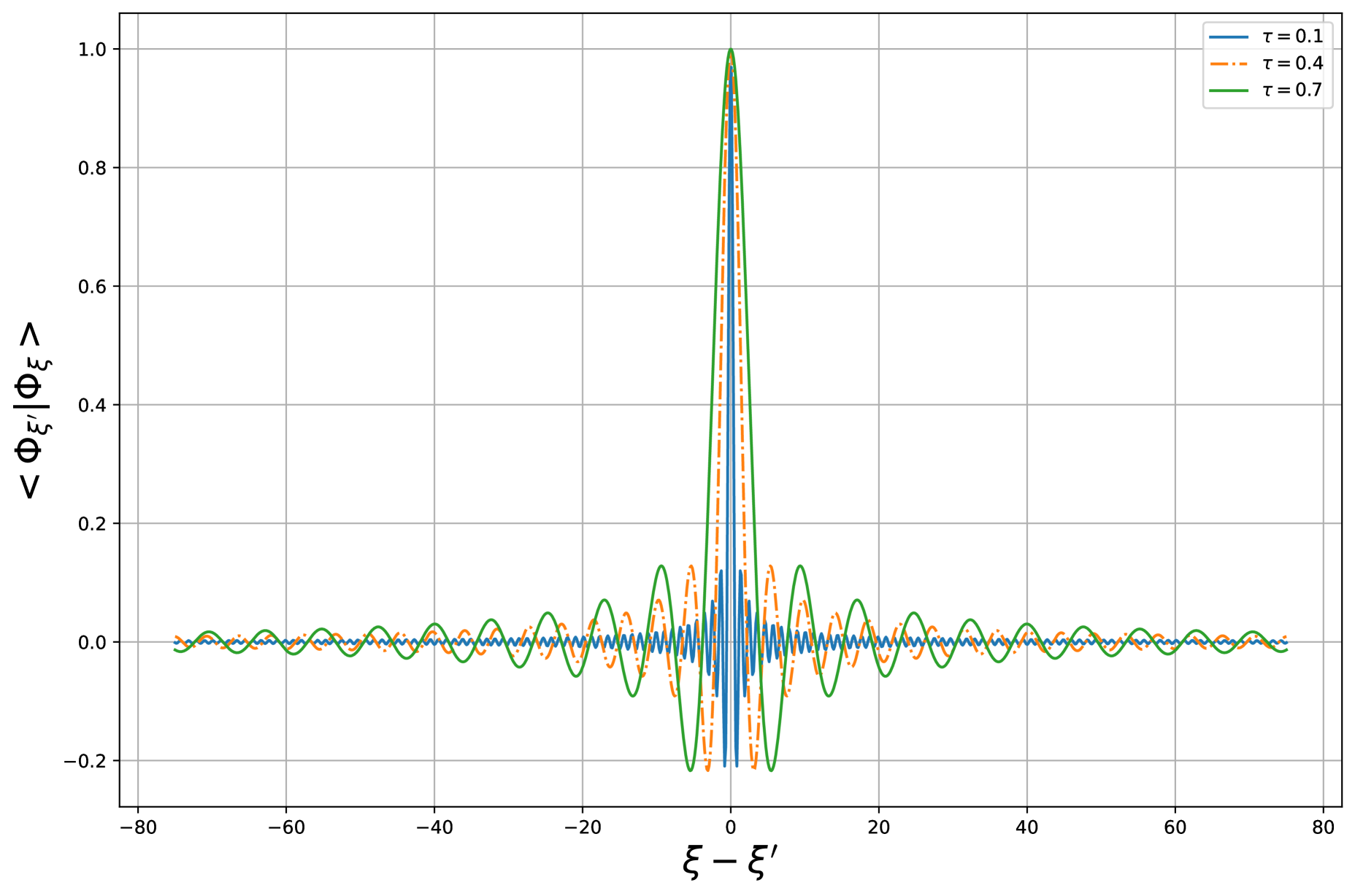
iv) The non-orthogonality relation:

	$\displaystyle\langle\Phi_{\xi^{\prime}}\|\Phi_{\xi}\rangle$	$\displaystyle=$	$\displaystyle\frac{\tau\sqrt{3}}{\pi}\int_{-\ell_{max}}^{+\ell_{max}}\frac{dx}{1-\tau x+\tau^{2}x^{2}}\exp\left(i\frac{2(\xi-\xi^{\prime})}{\tau\hbar\sqrt{3}}\left[\arctan\left(\frac{2\tau x-1}{\sqrt{3}}\right)+\frac{\pi}{6}\right]\right)$		(47)
		$\displaystyle=$	$\displaystyle\frac{\tau\hbar\sqrt{3}}{\pi(\xi-\xi^{\prime})}\sin\left(\pi\frac{\xi-\xi^{\prime}}{\tau\hbar\sqrt{3}}\right).$		(48)

This relation shows that, the normalized eigenstates (48) are no longer orthogonal. However, if one tends $(\xi-\xi^{\prime})\rightarrow\infty$ , these states become orthogonal

\displaystyle\lim_{(\xi-\xi^{\prime})\rightarrow\infty}\langle\Phi_{\xi^{\prime}}|\Phi_{\xi}\rangle=0.

(49)

For $(\xi-\xi^{\prime})\rightarrow 0,$ we have

\displaystyle\lim_{(\xi-\xi^{\prime})\rightarrow 0}\langle\Phi_{\xi^{\prime}}|\Phi_{\xi}\rangle=1.

(50)

These properties show that, the states $|\Phi_{\xi}\rangle$ are essentially Gaussians centered at $(\xi-\xi^{\prime})\rightarrow 0$ (see Figure 1). This indicates quantum fluctuations at this scale and these fluctuations increase with the deformed parameter $\tau$ .

Refer to caption — Figure 1: Variation of $\langle\Phi_{\xi^{\prime}}|\Phi_{\xi}\rangle$ versus $\xi-\xi^{\prime}$

v) The discreteness of the space:
Since the scalar product (45) vanishes in the limit $(\xi-\xi^{\prime})\rightarrow\infty$ , the states become orthogonal. The quantization follows from the condition

	$\displaystyle\pi\frac{\xi-\xi^{\prime}}{\tau\hbar\sqrt{3}}$	$\displaystyle=$	$\displaystyle n\pi$		(51)
	$\displaystyle\xi-\xi^{\prime}$	$\displaystyle=$	$\displaystyle\xi_{n}=\tau\hbar\sqrt{3}n,\quad n\in\mathbb{Z}.$		(52)

One notices that the spectrum of momentum operator $\hat{p}$ presents discrete values. From the letter equation, one sees that

\displaystyle\delta\xi_{n}=\xi_{n+1}-\xi_{n}=\tau\hbar\sqrt{3}=\sqrt{3}\Delta p_{min}.

(53)

With the above results (51) and (53) at hand, one confirms that the formal momentum eigenvectors $\big{|}\Phi_{\xi_{n}}\big{\rangle}=\big{|}\Phi_{\tau\hbar\sqrt{3}n}\big{\rangle}$ are physically accepted and relevant. One may be tempted to interpret the result (53) as if we are describing physics on a lattice in which each sites are spacing by the value $\sqrt{3}\Delta p_{min}$ . We interpret this as the space essentially having a discrete nature. Note that similar quantization of length was shown in the context of loop quantum gravity in [54, 55, 56, 57], albeit following a much more involved analysis, and perhaps under a stronger set of starting assumptions .

The wavefunctions (40) are square integrable functions (45), stable for the mean value of energy operator (46), have Gaussian distributions (49) (50) and have a discreteness nature (53). Consequently, the wavefunctions (40) are physically accepted and meaningful. Its representation in the quasi-Hermitian position-deformed Heisenberg algebra (33) are summarized by the following proposition:
Proposition 4.1: Given a Hilbert space $\mathcal{H}_{\tau}$ with the inner product $\langle.|.\rangle$ , the representation of quasi-Hermitian operators $\{\hat{x},\hat{p},\hat{h}\}$ in this space reads as follows

$\displaystyle\hat{x}\Phi_{\xi}(x)$	$\displaystyle=$	$\displaystyle x\Phi_{\xi}(x),$	(54)
$\displaystyle\hat{p}\Phi_{\xi}(x)$	$\displaystyle=$	$\displaystyle-i\hbar D_{x}\Phi_{\xi}(x)=\xi\Phi_{\xi}(x),$	(55)
$\displaystyle\hat{h}\Phi_{\xi}(x)$	$\displaystyle=$	$\displaystyle\left[-\frac{\hbar^{2}}{2m}D_{x}^{2}+V(x)\right]\Phi_{\xi}(x)=\left[-\frac{\hbar^{2}}{2m}\xi^{2}+V(x)\right]\Phi_{\xi}(x).$	(56)

Proof.

The proof follows from the equations (36) and (37). ∎

4.2 Fourier transform and its inverse representations

Since the states $|\Phi_{\xi}\rangle$ are physically meaningful and are well localized, one can determine its Fourier transform (FT) and its inverse representations by projecting an arbitrary state $|\Psi\rangle$ .
Definition 4.2: Let $\mathcal{S}\left(\mathbb{R}\right)$ be the Schwarz space which is dense in $\mathcal{H}=\mathcal{L}^{2}\left(\mathbb{R}\right)$ . Let $|\Psi\rangle\in\mathcal{S}\left(\mathbb{R}\right)$ , the FT denoted by $\mathcal{F}_{\tau}[\Psi]$ or $\Psi(\xi)$ is given by

\displaystyle\Psi(\xi)=\mathcal{F}_{\tau}[\Psi(x)](\xi)=\sqrt{\frac{\tau\sqrt{3}}{\pi}}\int_{-\ell_{max}}^{+\ell_{max}}\frac{\Psi(x)dx}{\sqrt{1-\tau x+\tau^{2}x^{2}}}e^{-i\frac{2\xi}{\tau\hbar\sqrt{3}}\left[\arctan\left(\frac{2\tau x-1}{\sqrt{3}}\right)+\frac{\pi}{6}\right]}.

(57)

The inverse FT is given by

\displaystyle\Psi(x)=\mathcal{F}_{\tau}^{-1}[\Psi(\xi)](x)=\frac{1}{\hbar\sqrt{4\pi\tau\sqrt{3}}}\int_{-\infty}^{+\infty}\frac{d\xi\Psi(\xi)}{\sqrt{1-\tau x+\tau^{2}x^{2}}}e^{i\frac{2\xi}{\tau\hbar\sqrt{3}}\left[\arctan\left(\frac{2\tau x-1}{\sqrt{3}}\right)+\frac{\pi}{6}\right]}.

(58)

Remarks: i) From the FT and inverse definitions follows the inequality

	$\displaystyle\|\Psi(\xi)\|^{2}$	$\displaystyle\leq$	$\displaystyle\sqrt{\frac{\tau\sqrt{3}}{\pi}}\int_{-\ell_{max}}^{+\ell_{max}}\frac{dx}{\sqrt{1-\tau x+\tau^{2}x^{2}}}\|\Psi(x)\|^{2}<\infty,$		(59)
	$\displaystyle\|\Psi(x)\|^{2}$	$\displaystyle\leq$	$\displaystyle\frac{1}{\hbar\sqrt{4\pi\tau\sqrt{3}}}\int_{-\infty}^{+\infty}\frac{d\xi}{\sqrt{1-\tau x+\tau^{2}x^{2}}}\|\Psi(\xi)\|^{2}<\infty.$		(60)

ii) As we have mentioned, the correction factor $1/\sqrt{1-\tau x+\tau^{2}x^{2}}$ enhances this FT and its inverse representations over the one previously obtained in [58]. Therefore, on this FT representation, the action of quasi-Hermitian operators will also be modified.

Properties 4.2: Let $|\Psi\rangle,|\Upsilon\rangle\in\mathcal{S}\left(\mathbb{R}\right),$ based on the definition of FT we have the following properties

	i)	$\displaystyle\mathcal{F}_{\tau}[\alpha\Psi(x)+\beta\Upsilon(x)](\xi)$	$\displaystyle=\alpha\Psi(\xi)+\beta\Upsilon(\xi),\quad\alpha,\beta\in\mathbb{C},$		(61)
	ii)	$\displaystyle\frac{1}{2\hbar\tau\sqrt{3}}\int_{-\infty}^{+\infty}\|\mathcal{F}_{\tau}[\Psi(x)](\xi)\|^{2}d\xi$	$\displaystyle=\int_{-\ell_{max}}^{+\ell_{max}}\|\Psi(x)\|^{2}dx,$		(62)

where the relations (i) and (ii) are respectively the linearity and the Parseval’s identity of FT. One may also deduce the convolution property of FT. For technical reasons, we arbitrary escape these aspects of the study and we hope to report elsewhere.

Proof.

i) For $\alpha,\beta\in\mathbb{C}$ , we have

$\displaystyle\mathcal{F}_{\tau}[\alpha\Psi(x)+\beta\Upsilon(x)](\xi)$	$\displaystyle=$	$\displaystyle\sqrt{\frac{\tau\sqrt{3}}{\pi}}\int_{-\ell_{max}}^{+\ell_{max}}\frac{\alpha\Psi(x)dx}{\sqrt{1-\tau x+\tau^{2}x^{2}}}e^{-i\frac{2\xi}{\tau\hbar\sqrt{3}}\left[\arctan\left(\frac{2\tau x-1}{\sqrt{3}}\right)+\frac{\pi}{6}\right]}$
		$\displaystyle+\sqrt{\frac{\tau\sqrt{3}}{\pi}}\int_{-\ell_{max}}^{+\ell_{max}}\frac{\beta\Upsilon(x)dx}{\sqrt{1-\tau x+\tau^{2}x^{2}}}e^{-i\frac{2\xi}{\tau\hbar\sqrt{3}}\left[\arctan\left(\frac{2\tau x-1}{\sqrt{3}}\right)+\frac{\pi}{6}\right]}$
	$\displaystyle=$	$\displaystyle\alpha\sqrt{\frac{\tau\sqrt{3}}{\pi}}\int_{-\ell_{max}}^{+\ell_{max}}\frac{\Psi(x)dx}{\sqrt{1-\tau x+\tau^{2}x^{2}}}e^{-i\frac{2\xi}{\tau\hbar\sqrt{3}}\left[\arctan\left(\frac{2\tau x-1}{\sqrt{3}}\right)+\frac{\pi}{6}\right]}$
		$\displaystyle+\beta\sqrt{\frac{\tau\sqrt{3}}{\pi}}\int_{-\ell_{max}}^{+\ell_{max}}\frac{\Upsilon(x)dx}{\sqrt{1-\tau x+\tau^{2}x^{2}}}e^{-i\frac{2\xi}{\tau\hbar\sqrt{3}}\left[\arctan\left(\frac{2\tau x-1}{\sqrt{3}}\right)+\frac{\pi}{6}\right]}$
	$\displaystyle=$	$\displaystyle\alpha\Psi(\xi)+\beta\Upsilon(\xi)$

ii) From the FT, we have

$\displaystyle\int_{-\infty}^{+\infty}\|\mathcal{F}_{\tau}[\Psi(x)](\xi)\|^{2}d\xi$	$\displaystyle=$	$\displaystyle\int_{-\infty}^{+\infty}\|\Psi(\xi)\|^{2}d\xi=\int_{-\infty}^{+\infty}\Psi(\xi)\Psi^{*}(\xi)d\xi$
	$\displaystyle=$	$\displaystyle\sqrt{\frac{\tau\sqrt{3}}{\pi}}\int_{-\infty}^{+\infty}d\xi\Psi(\xi)$
		$\displaystyle\times\left[\int_{-\ell_{max}}^{+\ell_{max}}\frac{\Psi^{*}(x)dx}{\sqrt{1-\tau x+\tau^{2}x^{2}}}e^{i\frac{2\xi}{\tau\hbar\sqrt{3}}\left[\arctan\left(\frac{2\tau x-1}{\sqrt{3}}\right)+\frac{\pi}{6}\right]}\right]$
	$\displaystyle=$	$\displaystyle\sqrt{\frac{\tau\sqrt{3}}{\pi}}\int_{-\ell_{max}}^{+\ell_{max}}\Psi^{*}(x)dx$
		$\displaystyle\times\int_{-\infty}^{+\infty}\frac{\Psi(\xi)d\xi}{\sqrt{1-\tau x+\tau^{2}x^{2}}}e^{i\frac{2\xi}{\tau\hbar\sqrt{3}}\left[\arctan\left(\frac{2\tau x-1}{\sqrt{3}}\right)+\frac{\pi}{6}\right]}$
	$\displaystyle=$	$\displaystyle 2\hbar\tau\sqrt{3}\int_{-\ell_{max}}^{+\ell_{max}}\Psi^{*}(x)\Psi(x)dx$
	$\displaystyle=$	$\displaystyle 2\hbar\tau\sqrt{3}\int_{-\ell_{max}}^{+\ell_{max}}\|\Psi(x)\|^{2}dx.$

∎

Proposition 4.2: Since the states $\Phi_{\xi}(x)$ are physically meaningful, there exist a new identity operator defined on $\mathcal{S}$

\displaystyle\int_{-\infty}^{+\infty}\frac{d\xi}{2\hbar\tau\sqrt{3}}|\xi\rangle\langle\xi|=\mathbb{I}_{\mathcal{S}}.

(63)

Proof.

Using equations (40) and (58), we have

$\displaystyle\langle x\|\Psi\rangle$	$\displaystyle=$	$\displaystyle\frac{1}{2\hbar\tau\sqrt{3}}\int_{-\infty}^{+\infty}d\xi\langle x\|\xi\rangle\langle\xi\|\Psi\rangle$
	$\displaystyle=$	$\displaystyle\frac{1}{\hbar\sqrt{4\pi\tau\sqrt{3}}}\int_{-\infty}^{+\infty}d\xi\Phi_{\xi}(x)\Psi(\xi)$
	$\displaystyle=$	$\displaystyle\frac{1}{\hbar\sqrt{4\pi\tau\sqrt{3}}}\int_{-\infty}^{+\infty}d\xi(1-\tau x+\tau^{2}x^{2})^{-\frac{1}{2}}\Psi(\xi)e^{i\frac{2\xi}{\tau\hbar\sqrt{3}}\left[\arctan\left(\frac{2\tau x-1}{\sqrt{3}}\right)+\frac{\pi}{6}\right]},$

which is equation (58). This confirms the claim that equation (63) is a correct expression for the identity which will play the role of the completeness relation of the momentum eigenstates in the derivation of the path-integral. ∎

Corollary 4.2: i) Let us consider arbitrary states $|\Xi\rangle,|\Theta\rangle\in\mathcal{S}\left(\mathbb{R}\right)$ , using the identity relation (63), their scalar product reads as follows

$\displaystyle\langle\Xi\|\Theta\rangle$	$\displaystyle=$	$\displaystyle\frac{1}{2\hbar\tau\sqrt{3}}\int_{-\infty}^{+\infty}d\xi\Xi^{*}(\xi)\Theta(\xi),$	(64)
	$\displaystyle=$	$\displaystyle\frac{1}{2\pi\hbar}\int_{-\infty}^{+\infty}d\xi\int_{-\ell_{max}}^{+\ell_{max}}\int_{-\ell_{max}}^{+\ell_{max}}\frac{dx^{\prime}}{\sqrt{1-\tau x^{\prime}+\tau^{2}x^{\prime 2}}}\frac{dx^{\prime}}{\sqrt{1-\tau x+\tau^{2}x^{2}}}$	(66)
		$\displaystyle\times e^{i\frac{2\xi}{\tau\hbar\sqrt{3}}\left[\arctan\left(\frac{2\tau x-1}{\sqrt{3}}\right)-\arctan\left(\frac{2\tau x^{\prime}-1}{\sqrt{3}}\right)\right]}\Xi(x^{\prime})\Theta(x).$	(66)

ii) The orthogonality of unit vector $|x\rangle$ is given by

$\displaystyle\langle x\|x^{\prime}\rangle$	$\displaystyle=$	$\displaystyle\int_{-\infty}^{+\infty}\frac{d\xi}{2\hbar\tau\sqrt{3}}\langle x\|\xi\rangle\langle\xi\|x^{\prime}\rangle=\int_{-\infty}^{+\infty}\frac{d\xi}{2\hbar\tau\sqrt{3}}\Phi_{\xi}(x)\Phi_{\xi}^{*}(x^{\prime})$	(67)
	$\displaystyle=$	$\displaystyle\frac{1}{2\pi\hbar}\int_{-\infty}^{+\infty}d\xi\exp\left(i\frac{2\xi}{\tau\hbar\sqrt{3}}\left[\arctan\left(\frac{2\tau x-1}{\sqrt{3}}\right)-\arctan\left(\frac{2\tau x^{\prime}-1}{\sqrt{3}}\right)\right]\right)$	(68)
	$\displaystyle=$	$\displaystyle\frac{\tau\sqrt{3}}{2}\delta\left(\arctan\left(\frac{2\tau x-1}{\sqrt{3}}\right)-\arctan\left(\frac{2\tau x^{\prime}-1}{\sqrt{3}}\right)\right)$	(69)
	$\displaystyle=$	$\displaystyle(1-\tau x+\tau^{2}x^{2})\delta(x-x^{\prime}).$	(70)

Proposition 4.3: From the definition of FT and its inverse, it is straightfoward to show that:

	i)	$\displaystyle\frac{d}{d\xi}\Psi(\xi)$	$\displaystyle=-i\frac{2}{\tau\hbar\sqrt{3}}\left[\arctan\left(\frac{2\tau x-1}{\sqrt{3}}\right)+\frac{\pi}{6}\right]\Psi(\xi),$		(71)
	ii)	$\displaystyle\frac{d}{dx}\Psi(x)$	$\displaystyle=\left(\tau\left(\frac{1}{2}-\tau x\right)+\frac{i\xi}{\hbar}\right)\frac{\Psi(x)}{1-\tau x+\tau^{2}x^{2}}.$		(72)

Lemma 4.2: The action of quasi-Hermitian operators (57) on $\Psi(\xi)$ reads as follows

$\displaystyle\hat{x}\Psi(\xi)$	$\displaystyle=$	$\displaystyle\frac{2}{\tau}\frac{\tan\left(i\frac{\tau\hbar\sqrt{3}}{2}\partial_{\xi}\right)}{\sqrt{3}+\tan\left(i\frac{\tau\hbar\sqrt{3}}{2}\partial_{\xi}\right)}\Psi(\xi),$	(73)
$\displaystyle\hat{p}\Psi(\xi)$	$\displaystyle=$	$\displaystyle\left(\xi-i2\hbar\tau\left(1-\frac{4\tan\left(i\frac{\tau\hbar\sqrt{3}}{2}\partial_{\xi}\right)}{\sqrt{3}+\tan\left(i\frac{\tau\hbar\sqrt{3}}{2}\partial_{\xi}\right)}\right)\right)\Psi(\xi),$	(74)
$\displaystyle\hat{h}\Psi(\xi)$	$\displaystyle=$	$\displaystyle\frac{1}{2m}\left(\xi-i2\hbar\tau\left(1-\frac{4\tan\left(i\frac{\tau\hbar\sqrt{3}}{2}\partial_{\xi}\right)}{\sqrt{3}+\tan\left(i\frac{\tau\hbar\sqrt{3}}{2}\partial_{\xi}\right)}\right)\right)^{2}\Psi(\xi)$	(76)
		$\displaystyle+V\left(\frac{2}{\tau}\frac{\tan\left(i\frac{\tau\hbar\sqrt{3}}{2}\partial_{\xi}\right)}{\sqrt{3}+\tan\left(i\frac{\tau\hbar\sqrt{3}}{2}\partial_{\xi}\right)}\right)\Psi(\xi).$	(76)

Proof.

Equation (71) is equivalent to

\displaystyle i\frac{\tau\hbar\sqrt{3}}{2}\frac{d}{d\xi}=\left[\arctan\left(\frac{2\tau x-1}{\sqrt{3}}\right)+\frac{\pi}{6}\right]=\left[\arctan\left(\frac{2\tau x-1}{\sqrt{3}}\right)+\arctan\left(\frac{1}{\sqrt{3}}\right)\right].

From the following relation [49]

\displaystyle\arctan\alpha+\arctan\beta=\arctan\left(\frac{\alpha+\beta}{1-\alpha\beta}\right),\quad\mbox{with}\quad\alpha\beta<1,

we deduce that

\displaystyle\tan\left[\arctan\left(\frac{2\tau x-1}{\sqrt{3}}\right)+\arctan\left(\frac{1}{\sqrt{3}}\right)\right]=\frac{\tau x\sqrt{3}}{2-\tau x}.

Therefore, the position operator $\hat{x}$ is represented as follows

	$\displaystyle\hat{x}$	$\displaystyle=$	$\displaystyle\frac{2}{\tau}\frac{\tan\left(i\frac{\tau\hbar\sqrt{3}}{2}\partial_{\xi}\right)}{\sqrt{3}+\tan\left(i\frac{\tau\hbar\sqrt{3}}{2}\partial_{\xi}\right)}\mathbb{I},$
	$\displaystyle x\Psi(\xi)$	$\displaystyle=$	$\displaystyle\frac{2}{\tau}\frac{\tan\left(i\frac{\tau\hbar\sqrt{3}}{2}\partial_{\xi}\right)}{\sqrt{3}+\tan\left(i\frac{\tau\hbar\sqrt{3}}{2}\partial_{\xi}\right)}\Psi(\xi).$

Using equation (72), the action of $\hat{p}$ on the quasi-representation (58) reads as follows

$\displaystyle\hat{p}\Psi(x)$	$\displaystyle=$	$\displaystyle\frac{-i\hbar}{\hbar\sqrt{4\pi\tau\sqrt{3}}}\int_{-\infty}^{+\infty}d\xi\Psi(\xi)$	(78)
		$\displaystyle\times D_{x}\left((1-\tau x+\tau^{2}x^{2})^{-1/2}e^{i\frac{2\xi}{\tau\hbar\sqrt{3}}\left[\arctan\left(\frac{2\tau x-1}{\sqrt{3}}\right)+\frac{\pi}{6}\right]}\right)$	(78)
	$\displaystyle=$	$\displaystyle\frac{1}{\hbar\sqrt{4\pi\tau\sqrt{3}}}\int_{-\infty}^{+\infty}\left(-i\hbar\tau\left(\frac{1}{2}-\tau x\right)+\xi\right)\Psi(\xi)$	(80)
		$\displaystyle\times\frac{d\xi}{\sqrt{1-\tau x+\tau^{2}x^{2}}}e^{i\frac{2\xi}{\tau\hbar\sqrt{3}}\left[\arctan\left(\frac{2\tau x-1}{\sqrt{3}}\right)+\frac{\pi}{6}\right]}.$	(80)

On the other hand, the action of $\hat{p}$ on the quasi-representation (58) reads as follows

	$\displaystyle\hat{p}\Psi(x)$	$\displaystyle=$	$\displaystyle\frac{1}{\hbar\sqrt{4\pi\tau\sqrt{3}}}\int_{-\infty}^{+\infty}\hat{p}\Psi(\xi)$		(82)
			$\displaystyle\times\frac{d\xi}{\sqrt{1-\tau x+\tau^{2}x^{2}}}e^{i\frac{2\xi}{\tau\hbar\sqrt{3}}\left[\arctan\left(\frac{2\tau x-1}{\sqrt{3}}\right)+\frac{\pi}{6}\right]}.$		(82)

By comparing equation (80) and equation (82), we obtain equation (74) of Lemma 3.2

	$\displaystyle\hat{p}\Psi(\xi)$	$\displaystyle=$	$\displaystyle\left(\xi-i\hbar\tau\left(\frac{1}{2}-\tau x\right)\right)\Psi(\xi)$
		$\displaystyle=$	$\displaystyle\left(\xi-i2\hbar\tau\left(1-\frac{4\tan\left(i\frac{\tau\hbar\sqrt{3}}{2}\partial_{\xi}\right)}{\sqrt{3}+\tan\left(i\frac{\tau\hbar\sqrt{3}}{2}\partial_{\xi}\right)}\right)\right)\Psi(\xi).$

The quasi-Hamiltonian is given by

	$\displaystyle\hat{h}\Psi(\xi)$	$\displaystyle=$	$\displaystyle\left(\frac{\hat{p}^{2}}{2m}+V(\hat{x})\right)\Psi(\xi)=\frac{1}{2m}\left(\xi-i2\hbar\tau\left(1-\frac{4\tan\left(i\frac{\tau\hbar\sqrt{3}}{2}\partial_{\xi}\right)}{\sqrt{3}+\tan\left(i\frac{\tau\hbar\sqrt{3}}{2}\partial_{\xi}\right)}\right)\right)^{2}\Psi(\xi)$
			$\displaystyle+V\left(\frac{2}{\tau}\frac{\tan\left(i\frac{\tau\hbar\sqrt{3}}{2}\partial_{\xi}\right)}{\sqrt{3}+\tan\left(i\frac{\tau\hbar\sqrt{3}}{2}\partial_{\xi}\right)}\right)\Psi(\xi).$

∎

Remark 4.2: From the limit $\tau\rightarrow 0$ in the last equations, we recover the ordinary representations in momentum space

$\displaystyle\lim_{\tau\rightarrow 0}\hat{x}\Psi(\xi)$	$\displaystyle=$	$\displaystyle i\hbar\partial_{\xi}\Psi(\xi),$	(83)
$\displaystyle\lim_{\tau\rightarrow 0}\hat{p}\Psi(\xi)$	$\displaystyle=$	$\displaystyle\xi\Psi(\xi),$	(84)
$\displaystyle\lim_{\tau\rightarrow 0}\hat{h}\Psi(\xi)$	$\displaystyle=$	$\displaystyle\left(\frac{\xi^{2}}{2m}+V\left(i\hbar\partial_{\xi}\right)\right)\Psi(\xi).$	(85)

5 Path integral

From the path integrals within this position-deformed Heisenberg algebra, we construct the propagator depending on the position-representation and on the Fourier transform and its inverse representations. We compute propagators and deduce the actions of a free particle.

5.1 Path integral in position-space representation

Definition 5.1: The path integral is defined by

\displaystyle\Phi_{\xi}(x,t)=\int_{-l_{max}}^{+l_{max}}dx^{\prime}K(x,x^{\prime},\Delta t)\Phi_{\xi}(x^{\prime},t^{\prime}),

(86)

where $K$ is the kernel in the Hamiltonian or the amplitude for a particle to propagate from the state with position $x^{\prime}$ to the state with position $x\,(x>x^{\prime})$ in a time interval $\Delta t=t-t^{\prime}$ [59, 60] and it is defined as

\displaystyle K(x,x^{\prime},\Delta t)=\langle x|e^{-\frac{i}{\hbar}\hat{h}\Delta t}|x^{\prime}\rangle.

(87)

Proposition 5.1: As easily checked the kernel (87) satisfies the following equations:

i)	$\displaystyle-\frac{\hbar^{2}}{2m}D_{x^{\prime}}^{2}K(x,x^{\prime},\Delta t)+V(x^{\prime})K(x,x^{\prime},\Delta t)=i\hbar\partial_{t}K(x,x^{\prime},\Delta t),$	(88)
ii)	$\displaystyle K(x,x^{\prime},0)=(1-\tau x+\tau^{2}x^{2})\delta(x-x^{\prime}),$	(89)
iii)	$\displaystyle\int_{-\ell_{max}}^{+\ell_{max}}dx^{\prime\prime}K(x,x^{\prime\prime},\Delta t_{1})K(x^{\prime\prime},x^{\prime},\Delta t_{2})=K(x,x^{\prime},\Delta t_{1}+\Delta t_{2}),$	(90)
iv)	$\displaystyle K^{\dagger}(x,x^{\prime},\Delta t)=K(x^{\prime},x,-\Delta t),$	(91)

where these equations are respectively: i) Schrödinger equation; ii) Initial condition; iii) Composition rule; iv) Unitarity.

Proof.

i) $i\hbar\partial_{t}K(x,x^{\prime},\Delta t)=\langle x|i\hbar\partial_{t}e^{-\frac{i}{\hbar}\hat{h}\Delta t}|x^{\prime}\rangle=\langle x|\hat{h}e^{-\frac{i}{\hbar}\hat{h}\Delta t}|x^{\prime}\rangle=\langle x|e^{-\frac{i}{\hbar}\hat{h}\Delta t}\hat{h}|x^{\prime}\rangle=\\ h(p,x^{\prime})\langle x|e^{-\frac{i}{\hbar}\hat{h}\Delta t}|x^{\prime}\rangle=h(p,x^{\prime})K(x,x^{\prime},\Delta t)=\left(-\frac{\hbar^{2}}{2m}D_{x^{\prime}}^{2}+V(x^{\prime})\right)K(x,x^{\prime},\Delta t)$ .
ii) $K(x,x^{\prime},0)=\langle x|x^{\prime}\rangle$ . Referring to the equation (72), we have $K(x,x^{\prime},0)=\langle x|x^{\prime}\rangle=(1-\tau x+\tau^{2}x^{2})\delta(x-x^{\prime})$ . iii) $K(x,x^{\prime},\Delta t_{1}+\Delta t_{2})=\langle x|e^{-\frac{i}{\hbar}\hat{h}(\Delta t_{1}+\Delta t_{2})}|x^{\prime}\rangle$
= $\langle x|e^{-\frac{i}{\hbar}\hat{h}\Delta t_{1}}e^{-\frac{i}{\hbar}\hat{h}\Delta t_{2}}|x^{\prime}\rangle=\int_{-\ell_{max}}^{+\ell_{max}}dx^{\prime\prime}\langle x|e^{-\frac{i}{\hbar}\hat{h}\Delta t_{1}}|x^{\prime\prime}\rangle\langle x^{\prime\prime}|e^{-\frac{i}{\hbar}\hat{h}\Delta t_{2}}|x^{\prime}\rangle$
$=\int_{-\ell_{max}}^{+\ell_{max}}dx^{\prime\prime}K(x,x^{\prime\prime},\Delta t_{1})K(x^{\prime\prime},x^{\prime},\Delta t_{2})$ . iv) $K^{\dagger}(x,x^{\prime},\Delta t)=\langle x^{\prime}|e^{\frac{i}{\hbar}\hat{h}\Delta t}|x\rangle=K^{\dagger}(x^{\prime},x,-\Delta t).$ ∎

Splitting the interval $t-t^{\prime}$ into N intervals of length $\epsilon=(t_{k}-t_{k-1})/N$ and inserting the completeness relations in (43) and (63), the propagator (87) becomes

	$\displaystyle K(x,x^{\prime},\Delta t)$	$\displaystyle=$	$\displaystyle\int_{-l_{max}}^{+l_{max}}\left(\prod_{k=1}^{N-1}dx_{k}\right)\int_{-\infty}^{+\infty}\left(\prod_{k=1}^{N}\frac{d\xi_{k}}{2\pi\hbar\tau\sqrt{3}}\right)$		(93)
			$\displaystyle\times\langle x_{k}\|\xi_{k}\rangle\langle\xi_{k}\|e^{-\frac{i}{\hbar}\epsilon\hat{h}}\|x_{k-1}\rangle.$		(93)

Recall that

$\displaystyle\langle x_{k}\|\xi_{k}\rangle$	$\displaystyle=$	$\displaystyle\Phi_{\xi_{k}}(x_{k})=\frac{\sqrt{\frac{\tau\sqrt{3}}{\pi}}}{\sqrt{1-\tau x_{k}+\tau^{2}x_{k}^{2}}}e^{\left(i\frac{2\xi_{k}}{\tau\hbar\sqrt{3}}\left[\arctan\left(\frac{2\tau x_{k}-1}{\sqrt{3}}\right)+\frac{\pi}{6}\right]\right)},$	(94)
$\displaystyle\langle\xi_{k}\|e^{-\frac{i}{\hbar}\epsilon\hat{h}}\|x_{k-1}\rangle$	$\displaystyle\simeq$	$\displaystyle e^{-\frac{i}{\hbar}\epsilon h(\xi_{k},x_{k-1})}\langle\xi_{k}\|x_{k-1}\rangle+\mathcal{O}(\epsilon^{2})$	(95)
	$\displaystyle\simeq$	$\displaystyle e^{-\frac{i}{\hbar}\epsilon h(\xi_{k},x_{k-1})}\Phi_{\xi_{k}}^{*}(x_{k-1})+\mathcal{O}(\epsilon^{2}).$	(96)

Proposition 5.2: Substituting equations (94) and (96) into equation (93) gives the discrete propagator

	$\displaystyle K_{disc}(x,x^{\prime},\Delta t)$	$\displaystyle=$	$\displaystyle\left[\int_{-l_{max}}^{+l_{max}}\left(\prod_{k=1}^{N-1}\frac{dx_{k}}{\sqrt{1-\tau x_{k}+\tau^{2}x_{k}^{2}}\sqrt{1-\tau x_{k-1}+\tau^{2}x_{k-1}^{2}}}\right)\right]$		(98)
			$\displaystyle\times\left[\int_{-\infty}^{+\infty}\left(\prod_{k=1}^{N}\frac{d\xi_{k}}{2\pi\hbar}\right)\right]e^{\frac{i}{\hbar}\epsilon\mathcal{S}_{disc}},$		(98)

where the discrete action $S_{disc}$ is given by

\displaystyle S_{disc}=\sum_{k=1}^{N-1}\frac{2\xi_{k}}{\tau\sqrt{3}}\left[\frac{\arctan\left(\frac{2\tau x_{k}-1}{\sqrt{3}}\right)-\arctan\left(\frac{2\tau x_{k-1}-1}{\sqrt{3}}\right)}{\epsilon}\right]-\sum_{k=1}^{N-1}h(\xi_{k},x_{k-1}).

(99)

Lemma 5.2: Taking $N\rightarrow\infty$ in equation (98), so that $\epsilon\rightarrow 0$ we obtain the continuous propagator as follows

\displaystyle K(x,x^{\prime},\Delta t)=\int\mathcal{D}x\mathcal{D}\xi e^{\frac{i}{\hbar}S},

(100)

where the integration measures $\mathcal{D}x$ and $\mathcal{D}\xi$ are defined as

\displaystyle\mathcal{D}x=\lim_{N\rightarrow\infty}\prod_{k=1}^{N-1}\frac{dx_{k}}{\sqrt{1-\tau x_{k}+\tau^{2}x_{k}^{2}}\sqrt{1-\tau x_{k-1}+\tau^{2}x_{k-1}^{2}}}\quad\mbox{and}\quad\mathcal{D}\xi=\lim_{N\rightarrow\infty}\prod_{k=1}^{N}\left(\frac{d\xi_{k}}{2\pi\hbar}\right).

(101)

and the continuous action $S$ is given by

\displaystyle S\left[x(t),x(t^{\prime})\right]

\displaystyle=

\displaystyle\int_{t^{\prime}}^{t}d\nu\left[\frac{\dot{x}(\nu)}{1-\tau x(\nu)+\tau^{2}x^{2}(\nu)}\xi(\nu)-h(\xi(\nu),x(\nu))\right],

(102)

where $\dot{x}(\nu)=dx/d\nu$ .

Remarks: i) As we can see, this formulation of path integral is quasi-similar to that in reference [49]. This similarity arises from the realization of this formulation within the quasi-Hermitian Heisenberg algebra, which is equivalent to the one used in [49]. Clairy, the quasi-Hermitian Hamiltonian variable $h(x,\xi)$ , which generalizes the pseudo-Hermitian one $H(x,\xi=\rho)$ used in [49] is also present in this path integral.
ii) Taking the limit $\tau\rightarrow 0$ in equation (35), the deformed propagator (100) is reduced to the ordinary one of Euclidean space such that

\displaystyle K^{0}(x,x^{\prime},\Delta t)=\int\lim_{N\rightarrow\infty}\prod_{k=1}^{N-1}dx_{k}\prod_{k=1}^{N}\left(\frac{d\xi_{k}}{2\pi\hbar}\right)e^{\frac{i}{\hbar}S^{0}},

(103)

where the undeformed action $S^{0}$ is given by

\displaystyle S^{0}\left[x(t),x(t^{\prime})\right]=\int_{t^{\prime}}^{t}d\nu\left[\dot{x}(\nu)\xi(\nu)-h(\xi(\nu),x(\nu))\right].

(104)

Theorem 5.2: It is straightforward to show that the following relations

\displaystyle K(x,x^{\prime},\Delta t)\leq K^{0}(x,x^{\prime},\Delta t)\implies S\leq S^{0}.

(105)

Proof.

The proof follows from a straightforward comparaison between equations (36) and (37) on one hand and, equations (102) and (104) on the other. ∎

It is well known that, the action in classical mechanics is a functional over paths that describe what is the motion of a system over a particular path. As we can see from this result (105), the deformed action $S$ is bounded by the ordinary one $S^{0}$ of classical mechanics. It makes sense to think of deformation effects as shortening the classical system’s path, which enables quick motion in this space.

The stationary path (102) is obtained by using the variational principle

\displaystyle\delta S=\delta\int_{t^{\prime}}^{t}d\nu L\left[\dot{x}(\nu),x(\nu)\right]=\int_{t^{\prime}}^{t}d\nu\left(\frac{\partial L}{\partial x(\nu)}\delta x(\nu)+\frac{\partial L}{\partial\dot{x}(\nu)}\delta\dot{x}(\nu)\right)=0,

(106)

where the Lagrangian $L$ of the system is given by

\displaystyle L\left[\dot{x}(\nu),x(\nu)\right]=\frac{\dot{x}(\nu)}{1-\tau x(\nu)+\tau^{2}x^{2}(\nu)}\xi(\nu)-h(\xi(\nu),x(\nu)).

(107)

The solutions of equation (106) generate the following differential equations

	$\displaystyle\dot{x}$	$\displaystyle=$	$\displaystyle(1-\tau x+\tau^{2}x^{2})\frac{\partial h}{\partial\xi}=\{x,\xi\}_{\tau}\frac{\partial h}{\partial\xi},$		(108)
	$\displaystyle\dot{\xi}$	$\displaystyle=$	$\displaystyle-(1-\tau x+\tau^{2}x^{2})\frac{\partial h}{\partial x}=-\{x,\xi\}_{\tau}\frac{\partial h}{\partial x},$		(109)

where $\{x,\xi\}_{\tau}=(1-\tau x+\tau^{2}x^{2})$ is the position-deformed Poisson bracket. By taking the limit $\tau\rightarrow 0$ , we recover the ordinary Hamilton equations of motion.

5.2 Path integral in Fourier transform and its inverse representions

Using the generalized Fourier transform and its inverse representations (57), (63) and taking into account equation (86), we have

$\displaystyle\Psi(\xi,t)$	$\displaystyle=$	$\displaystyle\sqrt{\frac{\tau\sqrt{3}}{\pi}}\int_{-\ell_{max}}^{+\ell_{max}}\frac{\Psi(x)dx}{\sqrt{1-\tau x+\tau^{2}x^{2}}}e^{-i\frac{2\xi}{\tau\hbar\sqrt{3}}\left[\arctan\left(\frac{2\tau x-1}{\sqrt{3}}\right)+\frac{\pi}{6}\right]}$	(112)
		$\displaystyle\times\int_{-l_{max}}^{+l_{max}}\frac{K(x,x^{\prime},\Delta t)}{\sqrt{1-\tau x^{\prime}+\tau^{2}x^{\prime 2}}}dx^{\prime}\frac{1}{\hbar\sqrt{4\pi\tau\sqrt{3}}}$
		$\displaystyle\times\int_{-\infty}^{+\infty}d\xi^{\prime}e^{i\frac{2\xi^{\prime}}{\tau\hbar\sqrt{3}}\left[\arctan\left(\frac{2\tau x^{\prime}-1}{\sqrt{3}}\right)+\frac{\pi}{6}\right]}\Psi(\xi^{\prime},t^{\prime}).$

This path integral can be rewritten as follows

\displaystyle\Psi(\xi,t)=\int_{-\infty}^{+\infty}d\xi^{\prime}\mathcal{K}(\xi,\xi^{\prime},\Delta t)\Psi(\xi^{\prime},t^{\prime}),

(113)

where $\mathcal{K}$ is the propagator in Fourier transform and its inverse representions for a particle to go from a state $\Psi(\xi^{\prime})$ to a state $\Psi(\xi)$ in a time interval $\Delta t$ is

$\displaystyle\mathcal{K}(\xi,\xi^{\prime},\Delta t)$	$\displaystyle=$	$\displaystyle\frac{1}{2\pi\hbar}\int_{-l_{max}}^{+l_{max}}\frac{dx}{\sqrt{1-\tau x+\tau^{2}x^{2}}}\frac{dx^{\prime}}{\sqrt{1-\tau x^{\prime}+\tau^{2}x^{\prime 2}}}$	(115)
		$\displaystyle\times e^{-i\frac{2}{\tau\hbar\sqrt{3}}\left[\xi\arctan\left(\frac{2\tau x-1}{\sqrt{3}}\right)-\xi^{\prime}\arctan\left(\frac{2\tau x^{\prime}-1}{\sqrt{3}}\right)\right]}K(x,x^{\prime},\Delta t),$	(115)
	$\displaystyle=$	$\displaystyle\frac{1}{2\pi\hbar}\int\mathcal{D}x\mathcal{D}\xi\frac{dx}{\sqrt{1-\tau x+\tau^{2}x^{2}}}\frac{dx^{\prime}}{\sqrt{1-\tau x^{\prime}+\tau^{2}x^{\prime 2}}}e^{\frac{i}{\hbar}\mathcal{S}},$	(116)

with the functional action $\mathcal{S}$ given by

\displaystyle\mathcal{S}(\xi,\xi^{\prime})=S-\frac{2}{\tau\sqrt{3}}\left[\xi\arctan\left(\frac{2\tau x-1}{\sqrt{3}}\right)-\xi^{\prime}\arctan\left(\frac{2\tau x^{\prime}-1}{\sqrt{3}}\right)\right].

(117)

5.3 Propagators for a free particle

The Hamiltonians of a free particle given by

\displaystyle\hat{h}_{fp}=\frac{\hat{p}^{2}}{2m}.

(118)

The propagator in position-represention in the time interval $\Delta t=t-t^{\prime}$ is given by

$\displaystyle K_{fp}(x,x^{\prime},\Delta t)$	$\displaystyle=$	$\displaystyle\langle x\|e^{-\frac{i}{\hbar}\frac{\hat{p}^{2}}{2m}\Delta t}\|x^{\prime}\rangle$	(119)
	$\displaystyle=$	$\displaystyle\frac{1}{2\pi\hbar\tau\sqrt{3}}\int_{-\infty}^{+\infty}d\xi e^{-\frac{i}{\hbar}\frac{\xi^{2}}{2m}\Delta t}\Phi_{\xi}(x)\Phi_{\xi}^{*}(x)$	(120)
	$\displaystyle=$	$\displaystyle\int_{-\infty}^{+\infty}\frac{d\xi}{2\pi\hbar}e^{\left(i\frac{2\xi}{\tau\hbar\sqrt{3}}\left[\arctan\left(\frac{2\tau x-1}{\sqrt{3}}\right)-\arctan\left(\frac{2\tau x^{\prime}-1}{\sqrt{3}}\right)\right]-\frac{i}{\hbar}\frac{\xi^{2}}{2m}\Delta t\right)}.$	(121)

Lemma 5.3: Completing this Gaussian integral (121), the deformed-propagator $K_{fp}$ , the deformed-action $S_{fp}$ and the deformed-kinetic energy $T$ read as follows

$\displaystyle K_{fp}(x,x^{\prime},\Delta t)$	$\displaystyle=$	$\displaystyle\sqrt{\frac{m}{2\pi\hbar i\Delta t}}e^{i\frac{2m}{\hbar 3\tau^{2}\Delta t}\left[\arctan\left(\frac{2\tau x-1}{\sqrt{3}}\right)-\arctan\left(\frac{2\tau x^{\prime}-1}{\sqrt{3}}\right)\right]^{2}},$	(122)
$\displaystyle S_{fp}$	$\displaystyle=$	$\displaystyle\frac{2m}{3\tau^{2}\Delta t}\left[\arctan\left(\frac{2\tau x-1}{\sqrt{3}}\right)-\arctan\left(\frac{2\tau x^{\prime}-1}{\sqrt{3}}\right)\right]^{2},$	(123)
$\displaystyle T$	$\displaystyle=$	$\displaystyle\frac{2m}{3\tau^{2}(\Delta t)^{2}}\left[\arctan\left(\frac{2\tau x-1}{\sqrt{3}}\right)-\arctan\left(\frac{2\tau x^{\prime}-1}{\sqrt{3}}\right)\right]^{2}.$	(124)

Proof.

See [49] for the proof of this Lemma 4.3. ∎

Taking the limit $\tau\rightarrow 0$ in equations (123), (122) and (124), these equations properly reduce to the well-known result in ordinary quantum mechanics for a free particle [59, 60] that is

$\displaystyle\lim_{\tau\rightarrow 0}K_{fp}(x,x^{\prime},\Delta t)$	$\displaystyle=$	$\displaystyle K_{fp}^{0}(x,x^{\prime},\Delta t)=\sqrt{\frac{m}{2\pi\hbar i\Delta t}}e^{\frac{i}{\hbar}\frac{m(x-x^{\prime})^{2}}{2\Delta t}},$	(125)
$\displaystyle\lim_{\tau\rightarrow 0}S_{fp}$	$\displaystyle=$	$\displaystyle S_{fp}^{0}=\frac{m}{2}\frac{(x-x^{\prime})^{2}}{\Delta t},$	(126)
$\displaystyle\lim_{\tau\rightarrow 0}T$	$\displaystyle=$	$\displaystyle T^{0}=\frac{m}{2}\frac{(x-x^{\prime})^{2}}{(\Delta t)^{2}}.$	(127)

Theorem 5.3: It is straightforward to show the following relations

\displaystyle K_{fp}(x,x^{\prime},\Delta t)\leq K_{fp}^{0}(x,x^{\prime},\Delta t)\implies S_{fp}\leq S_{fp}^{0}\implies T\leq T^{0}.

(128)

Proof.

The proof follows from a straightforward comparaison between equations of Lemma 4.3 and equations (125), (126) and (127) on the other. ∎

This indicates that the deformed propagator and actions of the free particle are dominated by the standard ones without quantum deformation. These results indicate that the quantum deformation effects in this space shortens the paths of particles, allowing them to move from one point to another in a short time. In one way or another, as one can see from equation (128), these results can be understood as free particles use low kinetic energies to travel faster in this deformed space. This confirms our recent results [46, 47] and strengthens the claim that the position deformed-algebra (33) induces strong deformation of the quantum levels allowing particles to jump from state to another with low energy transitions [46, 47].

Lemma 5.4: The propagator in the FT representation is given by

	$\displaystyle\mathcal{K}_{fp}(\xi,\xi^{\prime},\Delta t)$	$\displaystyle=$	$\displaystyle\frac{1}{2\pi\hbar}\sqrt{\frac{m}{2\hbar\pi i\Delta t}}\int_{-l_{max}}^{+l_{max}}\int_{-l_{max}}^{+l_{max}}\frac{dx}{\sqrt{1-\tau x+\tau^{2}x^{2}}}\frac{dx^{\prime}}{\sqrt{1-\tau x^{\prime}+\tau^{2}x^{\prime 2}}}$		(130)
			$\displaystyle\times e^{\frac{i}{\hbar}\mathcal{S}_{fp}},$		(130)

where $\mathcal{S}_{fp}$ is the corresponding action given by

\displaystyle\mathcal{S}_{fp}=S_{fp}-\frac{2}{\tau\sqrt{3}}\left[\xi\arctan\left(\frac{2\tau x-1}{\sqrt{3}}\right)-\xi^{\prime}\arctan\left(\frac{2\tau x^{\prime}-1}{\sqrt{3}}\right)\right].

(131)

Proof.

See [49] for the proof of this Lemma 4.4. ∎

6 Conclusion

The Hamiltonian operator in the study of dynamical quantum systems needs to be Hermitian. Therefore, the orthoganility of the Hamiltonian eigenbasis, the conservation of probability density, and the realism of the spectrum are all guaranteed by the Hamiltonian’s hermicity. Within a position-deformed Heisenberg algebra (20), we have demonstrated in the current study that a Hamiltonian operator with real spectrum is no longer Hermitian. Using a quasi-similarity transformation and a suitable positive-definite Dyson map (28) derived from a metric operator (22), we have determined the Hermicity of this operator. Next, we constructed Hilbert space representations associated with these quasi-Hermitian operators that form a quasi-Hermitian position deformed Heisenberg algebra (33). With the help of these representations we establish path integral formulations of any systems in this quasi-Hermitian algebra. The propagator is then considered as an example together with the appropriate action of a free particle. As a result of the Euclidean space’s deformation, we have demonstrated that the action that characterizes the system’s classical trajectory is constrained by the standard one of classical mechanics. Consequently, particles of this system travel quickly from one point to another with low kinetic energy.

Overall, the result achieved in this study is now identical to the result that was recently derived [49]. This result improves the previous one by the use of quasi-similarity transformation that restores the hermicity of the Hamiltonian operator. It is possible to interpret the expansion of the expression $(1-\tau x+\tau^{2}x^{2})^{-1/2}$ above the one obtained in [49] as an improvement of the wavefunction (40), the Fourier transform (57), and its inverse representations (58). The equivalence between the position-deformed Heisenberg algebra [49] and the quasi-Hermitian position deformed Heisenberg algebra (33) accounts for the similarity of path formulations of a free particle for both outcomes. In summary, the current paper’s finding, which was reached through the application of quasi-similarity, provides an additional method for obtaining the previous in [49].

Acknowledgments

LML acknowledges support from AIMS-RIC Grant.

References

[1] A. F. Ali, M. M. Khalil, E. C. Vagenas, Minimal length in quantum gravity and gravitational measurements, Europhysics Letters 112 (2) (2015) 20005
[2] M. Bishop, J. Contreras, J. Lee, D. Singleton, Reconciling a quantum gravity minimal length with lack of photon dispersion, Physics Letters B 816 (2021) 136265
[3] L. J. Garay, Quantum gravity and minimum length, International Journal of Modern Physics A 10 (02) (1995) 145–165
[4] S. Hossenfelder, Minimal length scale scenarios for quantum gravity, Living Reviews in Relativity 16 (1) (2013) 2.
[5] M. Maggiore, A generalized uncertainty principle in quantum gravity, Physics Letters B 304 (1-2) (1993) 65–69.
[6] M. Maggiore, The algebraic structure of the generalized uncertainty principle, Physics Letters B 319 (1-3) (1993) 83–86.
[7] M. Maggiore, Quantum groups, gravity, and the generalized uncertainty principle, Physical Review D 49 (10) (1994) 5182.
[8] L. Perivolaropoulos, Cosmological horizons, uncertainty principle, and maximum length quantum mechanics, Physical Review D 95 (10) (2017) 103523.
[9] S. Franchino-Vi˜nas, J. Relancio, Geometrizing the klein–gordon and dirac equations in doubly special relativity, Classical and Quantum Gravity 40 (5) (2023) 054001.
[10] Y. Sabri, K. Nouicer, Phase transitions of a gup-corrected schwarzschild black hole within isothermal cavities, Classical and Quantum Gravity 29 (21) (2012) 215015.
[11] A. N. Tawfik, A. M. Diab, A review of the generalized uncertainty principle, Reports on Progress in Physics 78 (12) (2015) 126001.
[12] P. Pedram, A higher order gup with minimal length uncertainty and maximal momentum ii: Applications, Physics Letters B 718 (2) (2012) 638–645.
[13] A. Kempf, G. Mangano, R. B. Mann, Hilbert space representation of the minimal length uncertainty relation, Physical Review D 52 (2) (1995) 1108.
[14] A. Kempf, G. Mangano, Minimal length uncertainty relation and ultraviolet regularization, Physical Review D 55 (12) (1997) 7909.
[15] L. Lawson, L. Gouba, G. Y. Avossevou, Two-dimensional noncommutative gravitational quantum well, Journal of Physics A: Mathematical and Theoretical 50 (47) (2017) 475202.
[16] S. Pramanik, A consistent approach to the path integral formalism of quantum mechanics based on the maximum length uncertainty, Classical and Quantum Gravity 39 (19) (2022) 195018.
[17] F. Dossa, G. Y. H. Avossevou, Deformed ladder operators for the generalized one-and two-mode squeezed harmonic oscillator in the presence of a minimal length, Theoretical and Mathematical Physics 211 (1) (2022) 532–544.
[18] F. Dossa, J. Koumagnon, J. Hounguevou, G. H. Avossevou, Two-dimensional dirac oscillator in a magnetic field in deformed phase space with minimal-length uncertainty relations, Theoretical and Mathematical Physics 213 (3) (2022) 1738–1746.
[19] L. M. Lawson, I. Nonkané, K. Sodoga, The damped harmonic oscillator at the classical limit of the snyder-de sitter space, arXiv preprint arXiv:2101.01223 (2021).
[20] A. Fring, L. Gouba, F. G. Scholtz, Strings from position-dependent noncommutativity, Journal of Physics A: Mathematical and Theoretical 43 (34) (2010) 345401.
[21] F. J. Dyson, Thermodynamic behavior of an ideal ferromagnet, Physical Review 102 (5) (1956) 1230.
[22] F. G. Scholtz, H. B. Geyer, F. Hahne, Quasi-Hermitian operators in quantum mechanics and the variational principle, Annals of Physics 213 (1) (1992) 74–101.
[23] C. M. Bender, Making sense of non-Hermitian hamiltonians, Reports on Progress in Physics 70 (6) (2007) 947.
[24] C. M. Bender, S. Boettcher, Real spectra in non-hermitian hamiltonians having p t symmetry, Physical review letters 80 (24) (1998) 5243.
[25] C. M. Bender, D. C. Brody, H. F. Jones, Complex extension of quantum mechanics, Physical review letters 89 (27) (2002) 270401.
[26] A. Mostafazadeh, Pseudo-hermiticity versus pt symmetry: the necessary condition for the reality of the spectrum of a non-hermitian hamiltonian, Journal of Mathematical Physics 43 (1) (2002) 205–214.
[27] F. Bagarello, J.-P. Gazeau, F. H. Szafraniec, M. Znojil, Non-selfadjoint operators in quantum physics: Mathematical aspects, John Wiley and Sons, 2015.
[28] J. dos Santos, F. d. S. Luiz, O. S. Duarte, M. H. Y. Moussa, Non-hermitian noncommutative quantum mechanics, The European Physical Journal Plus 134 (7) (2019) 332.
[29] J.-P. Antoine, C. Trapani, Operator (quasi-) similarity, quasi-hermitian operators and all that, in: Non-Hermitian Hamiltonians in Quantum Physics: Selected Contributions from the 15th International Conference on Non-Hermitian Hamiltonians in Quantum Physics, Palermo, Italy, 18-23 May 2015, Springer, 2016, pp. 45–65.
[30] J.-P. Antoine, C. Trapani, Some remarks on quasi-hermitian operators, Journal of Mathematical Physics 55 (1) (2014).
[31] E. Ergun, On the metric operator for a nonsolvable non-hermitian model, Reports on Mathematical Physics 75 (3) (2015) 403–416.
[32] Z. Ahmed, Pseudo-hermiticity of Hamiltonians under imaginary shift of the coordinate: real spectrum of complex potentials, Physics Letters A 290 (1-2) (2001) 19–22.
[33] L. Solombrino, Weak pseudo-hermiticity and antilinear commutant, Journal of Mathematical Physics 43 (11) (2002) 5439–5445.
[34] E. Elias N’Dolo, Non-hermitian two-dimensional harmonic oscillator in noncommutative phasespace, arXiv e-prints (2023) arXiv–2309. doi.org/10.48550/arXiv.2309.15247
[35] L. M. Lawson, K. Amouzouvi, K. Sodoga, K. Beltako, Position-dependent mass from noncommutativity and its statistical descriptions, International Journal of Geometric Methods in Modern Physics (2024)
[36] F. Bagarello, Uncertainty relation for non-hermitian operators, Journal of Physics A: Mathematical and Theoretical 56 (42) (2023) 425201.
[37] M. Znojil, Systematics of quasi-hermitian representations of non-hermitian quantum models, Annals of Physics 448 (2023) 169198.
[38] A. Das, Pseudo-hermitian quantum mechanics, in: Journal of Physics: Conference Series, Vol. 287, IOP Publishing, 2011, p. 012002.
[39] E. Ergun, et al., Finding of the metric operator for a quasi-hermitian model, Journal of Function Spaces 2013 (2013).
[40] A. Mostafazadeh, Pseudo-hermitian quantum mechanics with unbounded metric operators, Philosophical Transactions of the Royal Society A: Mathematical, Physical and Engineering Sciences 371 (1989) (2013) 20120050.
[41] A. Mostafazadeh, Pseudo-hermitian representation of quantum mechanics, International Journal of Geometric Methods in Modern Physics 7 (07) (2010) 1191–1306.
[42] J. Feinberg, R. Riser, Pseudo-hermitian random matrix models: General formalism, Nuclear Physics B 975 (2022) 115678.
[43] A. Mostafazadeh, Time-dependent pseudo-hermitian hamiltonians and a hidden geometric aspect of quantum mechanics, Entropy 22 (4) (2020) 471.
[44] R. Kretschmer, L. Szymanowski, Quasi-hermiticity in infinite-dimensional hilbert spaces, Physics Letters A 325 (2) (2004) 112–117.
[45] L. M. Lawson, Minimal and maximal lengths from position-dependent non-commutativity, Journal of Physics A: Mathematical and Theoretical 53 (11) (2020) 115303.
[46] L. M. Lawson, Position-dependent mass in strong quantum gravitational background fields, Journal of Physics A: Mathematical and Theoretical 55 (10) (2022) 105303.
[47] L. M. Lawson, Minimal and maximal lengths of quantum gravity from non-hermitian positiondependent noncommutativity, Scientific Reports 12 (1) (2022) 20650.
[48] L. M. Lawson, Statistical description of ideal gas at planck scale with strong quantum gravity measurement, Heliyon 8 (9) (2022).
[49] L. M. Lawson, P. K. Osei, K. Sodoga, F. Soglohu, Path integral in position-deformed heisenberg algebra with maximal length uncertainty, Annals of Physics 457 (2023) 169389.
[50] L. M. Lawson, P. K. Osei, Gazeau-klauder coherent states in position-deformed heisenberg algebra, Journal of Physics Communications 6 (8) (2022) 085016.
[51] A. Mostafazadeh, Hilbert space structures on the solution space of klein–gordon-type evolution equations, Classical and Quantum Gravity 20 (1) (2002) 155.
[52] M. Znojil, Quasi-hermitian formulation of quantum mechanics using two conjugate schroedinger equations, Axioms 12 (7) (2023) 644.
[53] A. Fring, M. H. Moussa, Unitary quantum evolution for time-dependent quasi-hermitian systems with nonobservable hamiltonians, Physical Review A 93 (4) (2016) 042114.
[54] C. Rovelli, L. Smolin, Discreteness of area and volume in quantum gravity, Nuclear Physics B 442 (3) (1995) 593–619.
[55] T. Thiemann, A length operator for canonical quantum gravity, Journal of Mathematical Physics 39 (6) (1998) 3372–3392.
[56] A. F. Ali, S. Das, E. C. Vagenas, Discreteness of space from the generalized uncertainty principle, Physics Letters B 678 (5) (2009) 497–499.
[57] S. Das, E. C. Vagenas, A. F. Ali, Discreteness of space from gup ii: relativistic wave equations, Physics Letters B 690 (4) (2010) 407–412.
[58] F. Bagarello, A concise review of pseudobosons, pseudofermions, and their relatives, Theoretical and Mathematical Physics 193 (2) (2017) 1680–1693.
[59] H. Kleinert, Path integrals in quantum mechanics, statistics, polymer physics, and financial markets, World scientific, 2009.
[60] D. C. Khandekar, D. K. S. L. K. Bhagwat, S. V. Lawande, K. Bhagwat, Path-integral methods and their applications, Allied Publishers, 2002