Hitting a New Low: The Unique 28 h Cessation of Accretion in the TESS Light Curve of YY Dra (DO Dra)

The Transiting Exoplanet Survey Satellite (TESS) observed YY Dra from 2019 December 25 until 2020 February 28 in Sectors 20 and 21. During these 65 days, it observed the system at a two-minute cadence across a broad bandpass ($\sim$600-1,000 nm) that covers the red and near-infrared spectrum, including the $R$ and $I$ bands. For a deeper description of TESS, see Ricker et al. (2015). Using the Python package lightkurve (Barentsen et al., 2020), we downloaded the TESS light curve, which has nearly continuous coverage with the exception of three $\sim$2-day gaps due to data downlinks.

The flux measurements from the TESS pipeline come in two forms: simple-aperture photometry (SAP) and pre-conditioned simple-aperture photometry (PDCSAP). The latter is a processed version of the former that attempts to remove systematic trends and the effects of blending. Although the elimination of these problems is desirable in principle, Littlefield et al. (2021) argued that the PDCSAP light curve of the IP TX Col removed an outburst that was present in the SAP light curve. With this issue in mind, we plotted the TESS PDCSAP and SAP fluxes as a function of the simultaneous Zwicky Transient Facility (ZTF) (Smith et al., 2019) $g$ flux, repeating the procedure separately for each sector. Our objective was to determine which version of the light curve better correlated with the contemporaneous ground-based data.

Following the exclusion of a single discrepant ZTF measurement, we determined that the SAP flux was much more strongly correlated with the ZTF flux than was the PDCSAP flux. The difference was especially pronounced during Sector 21, when the best-fit linear regressions had coefficients of determination of $r^{2}_{SAP}=0.92$ and $r^{2}_{PDC}=0.24$ for the SAP and PDCSAP light curves, respectively. These statistics indicate that 92% of the variation in the SAP light curve but only 24% of the variation in the PDCSAP data can be explained by the variations in the ZTF flux. During Sector 20, we found that $r^{2}_{SAP}=0.26$ and $r^{2}_{PDC}=0.02$. The higher values of $r^{2}$ during Sector 21 are probably because the range in brightness was much greater than in Sector 20. A visual inspection of the residuals from the linear fits confirmed that the low value of $r^{2}_{PDC}$ in both sectors was attributable to a weak correlation as opposed to a strong, but non-linear, relationship. Consequently, we elected to use the SAP light curve in our analysis.

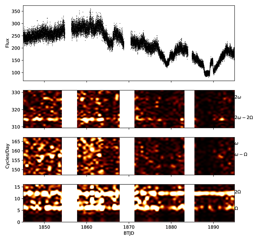
The top panel of Figure 1 shows the full TESS light curve, while Figure 2 shows selected segments to give a sense of the data quality. Throughout this paper, including Figure 1, we use the Barycentric TESS Julian Date (BTJD) convention to express time, which is defined as BTJD = BJD $-$ 2457000, where BJD is the Barycentric Julian Date in Barycentric Dynamical Time.

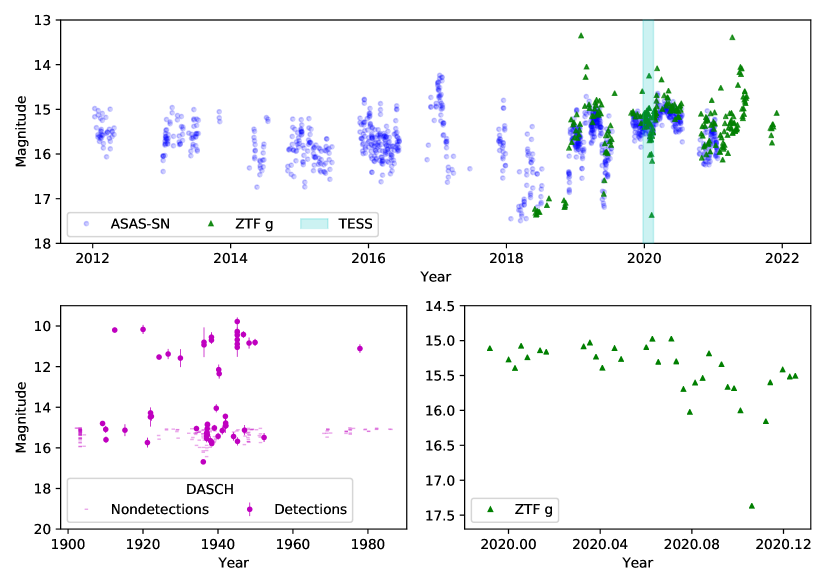
We compared the TESS light curve to a long-term light curve (Figure 3) assembled from the Harvard Digital Access to a Sky-Century at Harvard project (DASCH; Grindlay et al., 2009), the All-Sky Automated Survey for Supernovae (ASAS-SN; Shappee et al., 2014; Kochanek et al., 2017), and the ZTF. The DASCH light curve used the default quality flags of the project’s pipeline, and its magnitudes are appoximately equal to the Johnson $B$ band. We used only $g$ magnitudes from ASAS-SN and ZTF.

During the TESS observation, YY Dra was comparatively bright for the first 20 days ($g\sim 15.2$; Fig. 3), showing a slow, rising trend in the TESS data. However, for the remainder of the light curve, it generally exhibited a gradual fade, punctuated by three obvious dips (Figure 1, top panel). The slow fade began near BTJD=1865, leading into the first of the three dips at BTJD = 1868. Although YY Dra quickly recovered from this dip, the overall fading trend continued, and another, deeper dip took place at BTJD = 1878. The second dip consisted of a relatively rapid fade over $\sim 2.5$ d and thereafter recovered within 3.5 d, lasting about a week in total.

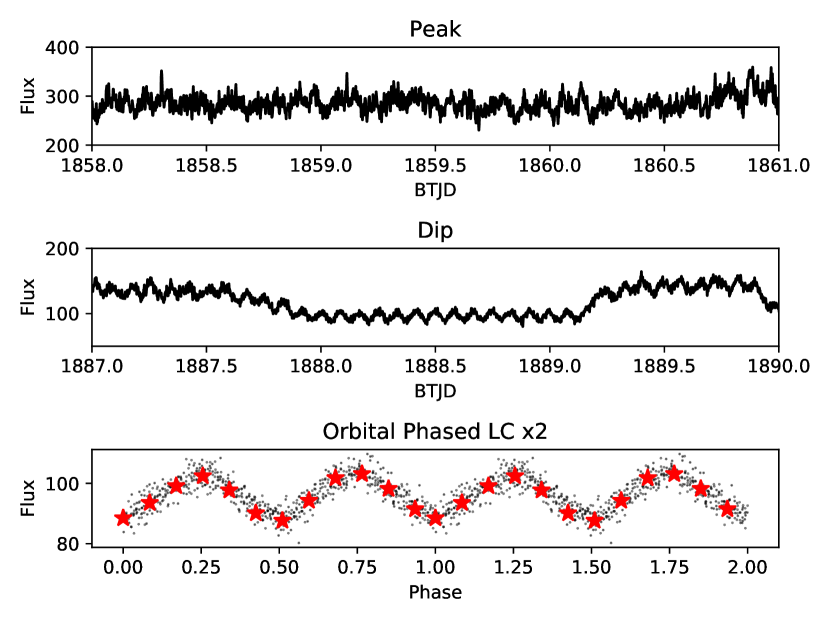
The third dip is the most remarkable feature of the light curve. Unlike the first two dips, its deepest portion is flat-bottomed, lasts for just 1.2 d, and was observed by ZTF to be $g=17.37\pm 0.12$, approximately 2 mag fainter than the beginning of the TESS light curve. The middle panel of Figure 2 shows a 3 d section of the light curve centered on this dip. The deepest part of the low state shows smooth, sinusoidal variation, the nature of which which we explore in Sec. 3.3. This low state began with a rapid 33% drop in brightness lasting eight hours at BTJD = 1888, and it ended with a burst that lasted for 16 h. After a rapid fade from the burst, YY Dra began a slow recovery, but it never completely recovered to its starting brightness during the TESS observation.

In the following subsections, we use power spectral analysis to gain insight into these behaviors.

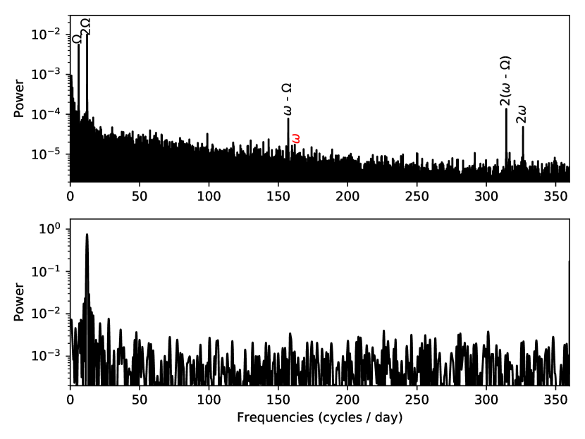
We computed a Lomb-Scargle power spectrum (Lomb, 1976; Scargle, 1982) to examine YY Dra’s periodic variations between 0.67 cycles d^-1 and 360 cycles d^-1. The $\Omega$, 2$\Omega$, 2($\omega$-$\Omega)$, and 2$\omega$ frequencies from Haswell et al. (1997) are easily identified in this power spectrum (Figure 4). Because of the relatively short TESS baseline, the measured periods from the power spectrum are statistically indistinguishable from those in Haswell et al. (1997).

The power spectrum of an IP contains important information about the system’s structure (Warner, 1986; Ferrario & Wickramasinghe, 1999; Murray et al., 1999). For example, Ferrario & Wickramasinghe (1999) computed theoretical optical power spectra for stream-fed and disk-fed IPs. They predicted that the spin period should tend to be very apparent during disk-fed accretion because the accretion disk encircles the entire white dwarf, providing each magnetic pole with a uniform reservoir of matter from which to accrete, regardless of the WD’s rotational phase. In stream-fed accretion, however, the white dwarf accretes from a fixed region in the binary rest frame: a single, focused point where the stream from the donor star encounters the magnetic field. In sharp contrast to disk-fed accretion, the accretion rate onto any one pole will vary with the WD’s rotation.

In YY Dra, stream-fed accretion could explain why there is a very conspicuous $\omega$-$\Omega$ and 2($\omega$-$\Omega)$ and a rather inconspicuous $\omega$. The Ferrario & Wickramasinghe (1999) models predict that stream-fed accretion will tend to shift power into $\omega$-$\Omega$ and its harmonics, and in YY Dra, the amplitudes of $\omega$-$\Omega$ and 2($\omega$-$\Omega)$ are much higher than $\omega$ and 2$\omega$. This distribution of power is not accounted for in the Ferrario & Wickramasinghe (1999) disk-fed models, but it is consistent with their stream-fed models, particularly at lower inclinations. Furthermore, the abrupt disappearance of $\Omega$ during a 28 h cessation of accretion during the TESS observation (Sec. 3.3) reveals that this frequency is produced by accretion (as opposed to the changing aspect of the donor star), which is consistent with a prediction by Ferrario & Wickramasinghe (1999) that stream-fed accretion will often shift power into $\Omega$.

Although we believe that the Ferrario & Wickramasinghe (1999) stream-fed accretion models offer the best explanation of the observed power spectrum, we also considered two other scenarios to account for YY Dra’s comparatively strong $\omega$-$\Omega$ and 2($\omega$-$\Omega)$ signals. The first was proposed by Warner (1986), who argued that stationary structures in the binary frame can reprocess X-rays into the optical at a frequency of $\omega$-$\Omega$; we presume that this effect could also produce a signal at 2($\omega$-$\Omega)$ if both poles participate in this process. However, one challenge with applying this scenario to YY Dra is that at its inclination of $i=42^{\circ}$ (Mateo et al., 1991), we would expect at least a modest amplitude modulation of the reprocessed optical radiation across the binary orbit, shifting power into the upper and lower orbital sidebands of both $\omega$-$\Omega$ and 2($\omega$-$\Omega)$(Warner, 1986). This predicted distribution of power is inconsistent with the observed power spectrum in Fig. 4 and suggests that the region in which the optical $\omega$-$\Omega$ and 2($\omega$-$\Omega)$ signals originate is uniformly visible across the orbit. While not absolutely conclusive, this reasoning disfavors reprocessed X-rays as the origin of $\omega$-$\Omega$ and 2($\omega$-$\Omega)$ in the TESS data.

Another alternative explanation that we considered involves the possibility of spiral structure within the accretion disk. Murray et al. (1999) computed theoretical power spectra for IPs in which spiral arms in the disk extend far enough inward to reach the disk’s inner rim. Similar to stream-fed accretion, this scenario would break the azimuthal symmetry of the accretion flow at the magnetospheric boundary, producing power at $\omega$-$\Omega$ and/or 2($\omega$-$\Omega)$. However, we disfavor this interpretation for two reasons. First, it seems unlikely that if a disk were present, the power at $\omega$-$\Omega$ and 2($\omega$-$\Omega)$ could dwarf that at $\omega$ and 2$\omega$. Second, we would not expect spiral disk structure to be present during quiescence in a CV with YY Dra’s 4 h orbital period. While spiral structure has been detected in IP Peg ($P_{orb}$ = 3.8 h) during its outbursts (Steeghs et al., 1997), the physical conditions in the disk during outburst—particularly its viscosity—are very different than in quiescence, and YY Dra’s faintness during the TESS observation rules out the possibility that the system possessed an outbursting disk.

We therefore conclude that YY Dra was predominantly stream-fed during these observations.

Figure 1 presents the evolution of the power spectrum over time and offers insight into the stability of YY Dra’s periodic variations as well as their dependence on the brightness of YY Dra. Throughout the observation, $\Omega$ and 2$\Omega$ were consistently the largest-amplitude signals in the two-dimensional power spectrum. Of the frequencies related to the WD’s rotation, 2($\omega$-$\Omega)$ consistently had the highest amplitude, while $\omega$-$\Omega$, $\omega$, and 2$\omega$ were not reliably detected above the noise in 0.5 day segments of the light curve. The amplitude of 2($\omega$-$\Omega)$ declines in the second half of the light curve, coinciding with YY Dra’s gradual fade.

During the 28 h long, flat-bottomed low state at BTJD=1888, no periodic variability is present, except for 2$\Omega$, and even the flickering appears to stop. We attribute this behavior to a cessation of accretion during which only ellipsoidal variations from the companion star are present in the light curve, as seen in other CVs during zero-accretion states (e.g. KR Aur; Rodríguez-Gil et al., 2020). The absence of accretion during this 28 h low state distinguishes it from the low state detected by Breus et al. (2017), during which YY Dra showed evidence of both ellipsoidal variations and additional variability at the orbital frequency, resulting in a double-humped orbital profile with unequal maxima; had accretion ceased altogether during the Breus et al. (2017) observations, we would expect to observe the maxima to have been equal. While episodes of negligible accretion have been identified in other magnetic CVs, our review of the literature suggests that states of insignificant accretion are extremely rare in IPs, as we discuss in Sec. 4.1.

Lastly, we unsuccessfully searched the two-dimensional power spectrum for evidence of transient periodic oscillations (TPOs), a phenomenon identified in YY Dra by Andronov et al. (2008). The TPOs in that study consisted of a mysterious signal near 86 cycles d^-1 whose frequency gradually decreased to 40 cycles d^-1 over the course of three nights. Because this phenomenon in the Andronov et al. (2008) dataset occurred at an elevated accretion rate ($\sim 1$ mag brighter than during the TESS observation), the lack of TPOs in the TESS data suggests that they are sensitive to the accretion rate.

The DASCH light curve spans from 1902 to 1986 and is by far the most sparsely sampled of the three datasets in Figure 3. However, it offers a unique look at YY Dra in the decades prior to its discovery. The DASCH data show no low states as deep as the one observed by both TESS and ZTF, although one observation (at magnitude $B=16.7$ in 1936) comes fairly close. The lack of deep low states could be attributable in part to the relatively shallow limiting magnitude of many of the photographic plates. Indeed, Figure 3 excludes 6,165 non-detections with limiting magnitudes brighter than 15, a threshold selected because it is too shallow to reach YY Dra’s quiescent brightness. Even the non-detections with comparatively deep limits cannot meaningfully distinguish between normal quiescent variability and a low state. Additionally, there are no observations during the early 1950s and late 1960s, so any low states during that interval would have gone undetected. Finally, while low states are elusive in the century-long light curve of YY Dra, the DASCH data do emphasize the bright, $>5$ mag outbursts of YY Dra, a distinguishing property noted by previous studies (e.g., Szkody et al., 2002).

While the DASCH data provide a partial glimpse of YY Dra’s behavior across the 20th century, the ASAS-SN and ZTF survey photometry provide significantly denser observational coverage during the past decade. The ASAS-SN and ZTF $g$ light curves, both of which overlap the TESS observations, are in excellent agreement with each another (Fig. 3, top panel). Although ASAS-SN has a longer baseline by six years, the ZTF data fill in some of the gaps in the ASAS-SN coverage. In 2018, YY Dra was regularly in a low state, dropping below $g\sim 17$, and while the exact duration of the low states is not clear, some of them could have lasted for months.

The ZTF data are especially critical because they include an observation of YY Dra during its deep low state (Figure 3). This single datum therefore establishes the magnitude of YY Dra when its accretion rate was negligible: $g=17.37\pm 0.12$. In the absence of any accretion, the optical luminosity of YY Dra should be composed of the stellar photospheres of the WD and the companion star. As such, the ZTF measurement should represent the minimum magnitude which YY Dra can appear, at least until the WD has cooled significantly. Inspecting Figure 3, it is evident that YY Dra spent much of 2018 in or near such a state.²²2Covington et al. (2022) examined archival observations of YY Dra from 2018 and identified a 3 mag fade in Swift ultraviolet UVW- and UVM-band observations that coincided with a non-detection of YY Dra in X-ray observations. Likewise, Shaw et al. (2020) found no X-ray emission in a 55.4 ks NuSTAR observation of YY Dra in July 2018. These findings provide independent support for a cessation of accretion onto the WD in 2018.

The minima of the ellipsoidal variations in Figure 2 are almost perfectly equal, making it difficult to identify which one corresponds to inferior conjunction of the donor star. However, the data can be reliably phased to the binary orbit using the Joshi (2013) orbital period and the Haswell et al. (1997) epoch of inferior conjunction.³³3 We converted the epoch of the Haswell et al. (1997) to Barycentric Julian Date in Barycentric Dynamical Time using routines in astropy. Because of the excellent precision of the Joshi (2013) orbital period (0.16537424(2) d), this trial ephemeris has an accumulated phase error of only $\pm 0.009$ at the time of the low state near BTJD=1888, so when the data are phased to it, the photometric minimum corresponding to inferior conjunction should be observed within $\pm 0.009$ orbital cycles of phase 0.0.

The phased data agree with this prediction. When phased to the aforementioned trial ephemeris, the closest minimum to phase 0.0 occurred at a nominal orbital phase of $\sim-0.02$. While this suggests that the Joshi (2013) uncertainty might have been slightly underestimated, the phasing of the deep-low-state light curve strongly supports our inference that ellipsoidal variations are responsible for the observed signal at 2$\Omega$.

Refining the orbital period slightly to 0.16537420(2) d corrects the phase shift from the Joshi (2013) orbital period. Adopting this revised orbital period, we offer an orbital ephemeris of

where $E$ is the integer cycle count.

Garnavich & Szkody (1988) searched for low states in three IPs in the Harvard plate collection: V1223 Sgr, FO Aqr, and AO Psc. They found that V1223 Sgr experienced a nearly decade-long low state whose depth was typically $\sim$1 mag but briefly exceeded 4 mag. Additionally, their analysis of AO Psc revealed a single $\sim$1 mag low state, lasting for at most several weeks. However, considering the difference in these time scales compared to YY Dra’s 28 h low state as well as the absence of contemporaneous time series photometry for the low states in the Harvard plates, it is difficult to compare the Garnavich & Szkody (1988) low states against the low state in the TESS light curve.

More recently, low-accretion states have been detected in several confirmed or suspected IPs, including V1323 Her (Andronov et al., 2014), FO Aqr (Littlefield et al., 2016; Kennedy et al., 2017), DW Cnc (Segura Montero et al., 2020), Swift J0746.3-1608 (Bernardini et al., 2019), J183221.56-162724.25 (J1832; Beuermann et al., 2022), and YY Dra itself (Breus et al., 2017), though as we noted in Sec. 3.3, the previously observed YY Dra low states do not show evidence of a cessation of accretion. Additionally, Covington et al. (2022) have identified low states in V1223 Sgr, V1025 Cen, V515 And, and RX J2133.7+5107, and they conclude that low states in IPs are more common than previously realized.

Detailed observations of these low states has revealed significant changes in the accretion geometry. FO Aqr is the best example of this, as optical (Littlefield et al., 2016, 2020), X-ray (Kennedy et al., 2017), and spectroscopic (Kennedy et al., 2020) studies have all agreed that the system’s mode of accretion changes at reduced mass-transfer rates. This is also true of DW Cnc and V515 And (Covington et al., 2022). With just one exception, these studies have not detected a total interruption of accretion during low states.

Of the other IPs that have been observed in low states, only in J1832 has the accretion rate been observed to decline to negligible levels. Similar to YY Dra, J1832 shows no variability related to the WD’s rotation during its deep low states (Beuermann et al., 2022), but J1832 has the added advantage of being a deeply eclipsing system. Beuermann et al. (2022) showed that when J1832 enters a deep low state, its optical eclipse depth becomes imperceptibly shallow, suggesting that there is no remaining accretion luminosity and hence no accretion. Due to gaps in ground-based observational coverage of J1832, it is unclear how long J1832’s deep low states last or how long it takes for the system to fall into one. In contrast, the TESS light curve of YY Dra firmly establishes the duration of the stoppage of accretion (28 h) as well as the length of the abrupt transitions into and out of that episode of negligible accretion (10 h and 2 h, respectively).

Interestingly, J1832 appears to be a persistently diskless IP (Beuermann et al., 2022), and we have argued that YY Dra’s power spectrum suggests that it too was diskless when its accretion ceased. This might be an important clue as to why the accretion rates of other IPs have not been observed to fall to negligible levels during their low states. A Keplerian disk is depleted at its viscous timescale, which can be days or even weeks, but in a diskless geometry, the lifetime of the accretion flow is much shorter (of order the free fall time between the system’s L1 point and the WD), so a cessation of mass transfer by the secondary would quickly result in a corresponding stoppage of accretion onto the WD.

More broadly, when looking at low states in other IPs, we see that they tend to last substantially longer (anywhere from months to years) than YY Dra’s 28 h deep low state. The low states in FO Aqr lasted 5-6 months in 2016, 4-5 months in 2017, and only 2-3 months in 2018 (Littlefield et al., 2020). Additionally, V1025 Cen (Covington et al., 2022; Littlefield et al., 2022) declined 2.5 magnitudes over the course of 4 years and remained in that low state for a little under 2 years. DW Cnc has significant gaps in the data, but it has shown a nearly 3 year low state with a depth of 2.3 mag (Covington et al., 2022). The lengths of these low states are substantially longer than those of YY Dra, underscoring the remarkable brevity of YY Dra’s deep low state.

Finally, Scaringi et al. (2017, 2021) examined low states of MV Lyr and TW Pic observed by Kepler and TESS, respectively. Although both systems are now suspected to be extremely low-field IPs, neither had been known to be magnetic. Scaringi et al. (2017, 2021) identified magnetically gated accretion episodes via the Spruit & Taam (1993) instability, resulting from a magnetic field strength so low that it produces observable effects (magnetically gated bursts) only during epochs of low accretion. In both MV Lyr and TW Pic, the low states tended to last for a number of days or even weeks, although one low state in TW Pic lasted for just over $\sim 1$ d. However, unlike the deep low state of YY Dra, TW Pic continued to accrete during this interval.

In conclusion, there is no reported precedent for a $\sim$day-long cessation in accretion in a confirmed IP. During a future episode of near-zero accretion, it should be possible to use optical spectra to search for Zeeman-split photospheric lines from the exposed WD in order to directly measure its magnetic-field strength.

Livio & Pringle (1994) and Hessman (2000) have theorized that star spots can pass over the inner hemisphere of a star and shrink the height of the companion star’s atmosphere, causing it to temporarily underfill its Roche lobe. Large star spots will distort the light curve of the companion’s ellipsoidal variations. When star spots are present, the shape of the ellipsoidal light curve would be distorted with a dip at certain orbital phases. If the star spots disappear, the dip should go away as well.

To search for evidence of such a change, we split the deep low state of the TESS light curve into two halves and phased both according to Equation 1. However, there are no statistically significant changes between the first and second halves of the deep low state. This result is perhaps unsurprising, given that each half of the deep low state encompasses only $\sim$3.5 binary orbits, which is too short a baseline to significantly boost the signal-to-noise ratio through phase-averaging the data. However, more precise measurements during a future cessation of accretion might be able to test more closely a change in the ellipsoidal light curve. A major benefit of performing such an analysis in a non-accreting IP (as opposed to a non-accreting polar) is that in a polar, the equality of $\omega$ and $\Omega$ makes it difficult to disentangle the secondary’s ellipsoidal variations from other sources of variability at the orbital frequency, such as accretion or thermal emission from hot spots on the WD surface (e.g., as observed for the low-state polar LSQ1725-64; Fuchs et al., 2016).

Although the TESS data therefore cannot test the starspot model, they do offer a helpful clue as to when mass transfer from the donor (as distinguished from the instantaneous accretion onto the WD) stopped. In a disk-fed geometry, a disk will dissipate at its viscous timescale, which can be several weeks (or longer) at low mass-transfer rates. In such a system, a disk can therefore be present even if it is not being replenished with mass from the donor star, and the only observable sign that the secondary is not transferring mass would be the disappearance of the hotspot where the accretion stream impacts the rim of the disk. Had YY Dra been accreting from a disk during the TESS observation, we would have expected to detect the hotspot as a contribution to $\Omega$ and perhaps its harmonics in the power spectrum, and its disappearance would have been observable in the 2D power spectrum. No such changes are observed. However, in a stream-fed geometry, there is only a short lag between a cessation of mass loss by the companion and the resulting interruption of accretion on to the WD.

Finally, it is worth noting that the flare at the end of the deep low state bears at least some resemblance to the behavior of the apparently non-magnetic VY Scl system KR Aur during its deep low states, when as in YY Dra ellipsoidal variability dominates the light curve (Rodríguez-Gil et al., 2020). However, in KR Aur, the flaring episodes appear to be short, lasting for tens of minutes as opposed to 0.7 d observed in YY Dra. Moreover, one of the longer low-state flares in KR Aur showed evidence of a quasi-periodicity, while the flare in YY Dra showed no significant periodicity other than the underlying ellipsoidal variations.

References

- Andronov et al. (2008) Andronov, I. L., Chinarova, L. L., Han, W., Kim, Y., & Yoon, J. N. 2008, A&A, 486, 855, doi: 10.1051/0004-6361:20079056
- Andronov et al. (2014) Andronov, I. L., Dubovsky, P., Yoon, J.-N., & Kim, Y. 2014, The Astronomer’s Telegram, 5944, 1
- Astropy Collaboration et al. (2013) Astropy Collaboration, Robitaille, T. P., Tollerud, E. J., et al. 2013, A&A, 558, A33, doi: 10.1051/0004-6361/201322068
- Astropy Collaboration et al. (2018) Astropy Collaboration, Price-Whelan, A. M., SipHocz, B. M., et al. 2018, AJ, 156, 123, doi: 10.3847/1538-3881/aabc4f
- Bailer-Jones et al. (2021) Bailer-Jones, C. A. L., Rybizki, J., Fouesneau, M., Demleitner, M., & Andrae, R. 2021, AJ, 161, 147, doi: 10.3847/1538-3881/abd806
- Barentsen et al. (2020) Barentsen, G., Hedges, C., Vinícius, Z., et al. 2020, KeplerGO/lightkurve: v2.0b3, v2.0b3, Zenodo, doi: 10.5281/zenodo.1181928
- Bernardini et al. (2019) Bernardini, F., de Martino, D., Mukai, K., & Falanga, M. 2019, MNRAS, 484, 101, doi: 10.1093/mnras/sty3499
- Beuermann et al. (2022) Beuermann, K., Breitenstein, P., & Schwab, E. 2022, A&A, 657, A101, doi: 10.1051/0004-6361/202141585
- Breus et al. (2017) Breus, V. V., Andronov, I. L., Yoon, J.-N., & Dubovský, P. 2017, The Astronomer’s Telegram, 10477, 1
- Buckley et al. (1997) Buckley, D. A. H., Haberl, F., Motch, C., et al. 1997, MNRAS, 287, 117, doi: 10.1093/mnras/287.1.117
- Buckley et al. (1995) Buckley, D. A. H., Sekiguchi, K., Motch, C., et al. 1995, MNRAS, 275, 1028, doi: 10.1093/mnras/275.4.1028
- Covington et al. (2022) Covington, A. E., Shaw, A. W., Mukai, K., et al. 2022, arXiv e-prints, arXiv:2202.08365. https://arxiv.org/abs/2202.08365
- Drake et al. (2014) Drake, A. J., Graham, M. J., Djorgovski, S. G., et al. 2014, ApJS, 213, 9, doi: 10.1088/0067-0049/213/1/9
- Ferrario & Wickramasinghe (1999) Ferrario, L., & Wickramasinghe, D. T. 1999, MNRAS, 309, 517, doi: 10.1046/j.1365-8711.1999.02860.x
- Fuchs et al. (2016) Fuchs, J. T., Dunlap, B. H., Dennihy, E., et al. 2016, MNRAS, 462, 2382, doi: 10.1093/mnras/stw1759
- Garnavich & Szkody (1988) Garnavich, P., & Szkody, P. 1988, PASP, 100, 1522, doi: 10.1086/132358
- Grindlay et al. (2009) Grindlay, J., Tang, S., Simcoe, R., et al. 2009, in Astronomical Society of the Pacific Conference Series, Vol. 410, Preserving Astronomy’s Photographic Legacy: Current State and the Future of North American Astronomical Plates, ed. W. Osborn & L. Robbins, 101
- Haswell et al. (1997) Haswell, C. A., Patterson, J., Thorstensen, J. R., Hellier, C., & Skillman, D. R. 1997, ApJ, 476, 847, doi: 10.1086/303630
- Hellier (2001) Hellier, C. 2001, Cataclysmic Variable Stars (Springer)
- Hessman (2000) Hessman, F. V. 2000, New A Rev., 44, 155, doi: 10.1016/S1387-6473(00)00030-0
- Hunter (2007) Hunter, J. D. 2007, Computing in Science and Engineering, 9, 90, doi: 10.1109/MCSE.2007.55
- Jayasinghe et al. (2018) Jayasinghe, T., Kochanek, C. S., Stanek, K. Z., et al. 2018, MNRAS, 477, 3145, doi: 10.1093/mnras/sty838
- Jayasinghe et al. (2019) Jayasinghe, T., Stanek, K. Z., Kochanek, C. S., et al. 2019, MNRAS, 486, 1907, doi: 10.1093/mnras/stz844
- Joshi et al. (2016) Joshi, A., Pandey, J. C., Singh, K. P., & Agrawal, P. C. 2016, ApJ, 830, 56, doi: 10.3847/0004-637X/830/2/56
- Joshi (2013) Joshi, V. 2013, in Astronomical Society of India Conference Series, Vol. 9, Astronomical Society of India Conference Series, 80
- Kennedy et al. (2017) Kennedy, M. R., Garnavich, P. M., Littlefield, C., et al. 2017, MNRAS, 469, 956, doi: 10.1093/mnras/stx880
- Kennedy et al. (2020) —. 2020, MNRAS, 495, 4445, doi: 10.1093/mnras/staa1415
- Kochanek et al. (2017) Kochanek, C. S., Shappee, B. J., Stanek, K. Z., et al. 2017, PASP, 129, 104502, doi: 10.1088/1538-3873/aa80d9
- Littlefield et al. (2022) Littlefield, C., Lasota, J.-P., Hameury, J.-M., et al. 2022, ApJ, 924, L8, doi: 10.3847/2041-8213/ac4262
- Littlefield et al. (2021) Littlefield, C., Scaringi, S., Garnavich, P., et al. 2021, AJ, 162, 49, doi: 10.3847/1538-3881/ac062b
- Littlefield et al. (2016) Littlefield, C., Garnavich, P., Kennedy, M. R., et al. 2016, ApJ, 833, 93, doi: 10.3847/1538-4357/833/1/93
- Littlefield et al. (2020) —. 2020, ApJ, 896, 116, doi: 10.3847/1538-4357/ab9197
- Livio & Pringle (1994) Livio, M., & Pringle, J. E. 1994, ApJ, 427, 956, doi: 10.1086/174202
- Lomb (1976) Lomb, N. R. 1976, Ap&SS, 39, 447, doi: 10.1007/BF00648343
- Mateo et al. (1991) Mateo, M., Szkody, P., & Garnavich, P. 1991, ApJ, 370, 370, doi: 10.1086/169823
- Murray et al. (1999) Murray, J. R., Armitage, P. J., Ferrario, L., & Wickramasinghe, D. T. 1999, MNRAS, 302, 189, doi: 10.1046/j.1365-8711.1999.02110.x
- Norton et al. (2004) Norton, A. J., Somerscales, R. V., & Wynn, G. A. 2004, in Astronomical Society of the Pacific Conference Series, Vol. 315, IAU Colloq. 190: Magnetic Cataclysmic Variables, ed. S. Vrielmann & M. Cropper, 216. https://arxiv.org/abs/astro-ph/0301351
- Patterson (1994) Patterson, J. 1994, PASP, 106, 209, doi: 10.1086/133375
- Patterson & Eisenman (1987) Patterson, J., & Eisenman, N. 1987, Information Bulletin on Variable Stars, 3079, 1
- Patterson et al. (1992) Patterson, J., Schwartz, D. A., Pye, J. P., et al. 1992, ApJ, 392, 233, doi: 10.1086/171421
- Patterson & Szkody (1993) Patterson, J., & Szkody, P. 1993, PASP, 105, 1116, doi: 10.1086/133289
- Patterson et al. (1982) Patterson, J., Schwartz, D. A., Bradt, H., et al. 1982, in Bulletin of the American Astronomical Society, Vol. 14, 618
- Ricker et al. (2015) Ricker, G. R., Winn, J. N., Vanderspek, R., et al. 2015, Journal of Astronomical Telescopes, Instruments, and Systems, 1, 014003, doi: 10.1117/1.JATIS.1.1.014003
- Rodríguez-Gil et al. (2020) Rodríguez-Gil, P., Shahbaz, T., Torres, M. A. P., et al. 2020, MNRAS, 494, 425, doi: 10.1093/mnras/staa612
- Scargle (1982) Scargle, J. D. 1982, ApJ, 263, 835, doi: 10.1086/160554
- Scaringi et al. (2017) Scaringi, S., Maccarone, T. J., D’Angelo, C., Knigge, C., & Groot, P. J. 2017, Nature, 552, 210, doi: 10.1038/nature24653
- Scaringi et al. (2021) Scaringi, S., de Martino, D., Buckley, D. A. H., et al. 2021, Nature Astronomy, doi: 10.1038/s41550-021-01494-x
- Schwarz et al. (2007) Schwarz, R., Schwope, A. D., Staude, A., et al. 2007, A&A, 473, 511, doi: 10.1051/0004-6361:20077684
- Segura Montero et al. (2020) Segura Montero, O., Ramírez, S. H., & Echevarría, J. 2020, MNRAS, 494, 4110, doi: 10.1093/mnras/staa856
- Shappee et al. (2014) Shappee, B. J., Prieto, J. L., Grupe, D., et al. 2014, ApJ, 788, 48, doi: 10.1088/0004-637X/788/1/48
- Shaw et al. (2020) Shaw, A. W., Heinke, C. O., Mukai, K., et al. 2020, MNRAS, 498, 3457, doi: 10.1093/mnras/staa2592
- Smith et al. (2019) Smith, K. W., Williams, R. D., Young, D. R., et al. 2019, Research Notes of the American Astronomical Society, 3, 26, doi: 10.3847/2515-5172/ab020f
- Spruit & Taam (1993) Spruit, H. C., & Taam, R. E. 1993, ApJ, 402, 593, doi: 10.1086/172162
- Steeghs et al. (1997) Steeghs, D., Harlaftis, E. T., & Horne, K. 1997, MNRAS, 290, L28, doi: 10.1093/mnras/290.2.L28
- Szkody et al. (2002) Szkody, P., Nishikida, K., Erb, D., et al. 2002, AJ, 123, 413, doi: 10.1086/324733
- Tsesevich (1934) Tsesevich, W. 1934, Perem. Zvezdy, 4, 291
- Virnina (2011) Virnina, N. A. 2011, Open European Journal on Variable Stars, 133, 1. https://arxiv.org/abs/1102.1271
- Warner (1986) Warner, B. 1986, MNRAS, 219, 347, doi: 10.1093/mnras/219.2.347
- Warner (1995) —. 1995, Cambridge Astrophysics Series, 28