yearnumberscity
Michael Kowalczyk
Jin-Yi Cai
Holant Problems for Regular Graphs with Complex Edge Functions
Abstract.
We prove a complexity dichotomy theorem for Holant Problems on -regular graphs with an arbitrary complex-valued edge function. Three new techniques are introduced: (1) higher dimensional iterations in interpolation; (2) Eigenvalue Shifted Pairs, which allow us to prove that a pair of combinatorial gadgets in combination succeed in proving #P-hardness; and (3) algebraic symmetrization, which significantly lowers the symbolic complexity of the proof for computational complexity. With holographic reductions the classification theorem also applies to problems beyond the basic model.
Key words and phrases:
Computational complexity1991 Mathematics Subject Classification:
F.2.11. Introduction
In this paper we consider the following subclass of Holant Problems [FOCS08, TAMC]. An input regular graph is given, where every is labeled with a (symmetric) edge function . The function takes 0-1 inputs from its incident nodes and outputs arbitrary values in . The problem is to compute the quantity .
Holant Problems are a natural class of counting problems. As introduced in [FOCS08, TAMC], the general Holant Problem framework can encode all Counting Constraint Satisfaction Problems (#CSP). This includes special cases such as weighted Vertex Cover, Graph Colorings, Matchings, and Perfect Matchings. The subclass of Holant Problems in this paper can also be considered as (weighted) -homomorphism (or -coloring) problems [BulatovG05, Homomorphisms, acyclic, DyerG00, Goldberg-4, Hell] with an arbitrary symmetric complex matrix , however restricted to regular graphs as input. E.g., Vertex Cover is the case when . When the matrix is a 0-1 matrix, it is called unweighted. Dichotomy theorems (i.e., the problem is either in or #P-hard, depending on ) for unweighted -homomorphisms with undirected graphs and directed acyclic graphs are given in [DyerG00] and [acyclic] respectively. A dichotomy theorem for any symmetric matrix with non-negative real entries is proved in [BulatovG05]. Goldberg et al. [Goldberg-4] proved a dichotomy theorem for all real symmetric matrices . Finally, Cai, Chen, and Lu have proved a dichotomy theorem for all complex symmetric matrices [Homomorphisms].
The crucial difference between Holant Problems and #CSP is that in #CSP, Equality functions of arbitrary arity are presumed to be present. In terms of -homomorphism problems, this means that the input graph is allowed to have vertices of arbitrarily high degrees. This may appear to be a minor distinction; in fact it has a major impact on complexity. It turns out that if Equality gates of arbitrary arity are freely available in possible inputs then it is technically easier to prove #P-hardness. Proofs of previous dichotomy theorems make extensive use of constructions called thickening and stretching. These constructions require the availability of Equality gates of arbitrary arity (equivalently, vertices of arbitrarily high degrees) to carry out. Proving #P-hardness becomes more challenging in the degree restricted case. Furthermore there are indeed cases within this class of counting problems where the problem is #P-hard for general graphs, but solvable in when restricted to 3-regular graphs.
We denote the (symmetric) edge function by , where , and . Functions will also be called gates or signatures. (For Vertex Cover, the function corresponding to is the Or gate, and is denoted by the signature .) In this paper we give a dichotomy theorem for the complexity of Holant Problems on 3-regular graphs with arbitrary signature , where . First, if , the Holant Problem is easily solvable in . Assuming we may normalize and assume . Our main theorem is as follows:
Theorem 1.1.
Suppose , and let , . Then the Holant Problem on 3-regular graphs with is #P-hard except in the following cases, for which the problem is in .
-
(1)
.
-
(2)
.
-
(3)
and .
-
(4)
and .
If we restrict the input to planar 3-regular graphs, then these four categories are solvable in , as well as a fifth category . The problem remains #P-hard in all other cases. 111Technically, computational complexity involving complex or real numbers should, in the Turing model, be restricted to computable numbers. In other models such as the Blum-Shub-Smale model [BSS] no such restrictions are needed. Our results are not sensitive to the exact model of computation. ∎
These results can be extended to -regular graphs (we detail how this is accomplished in a forthcoming work). One can also use holographic reductions [HA_FOCS] to extend this theorem to more general Holant Problems.
In order to achieve this result, some new proof techniques are introduced. To discuss this we first take a look at some previous results. Valiant [Valiant79b, Valiant:sharpP] introduced the powerful technique of interpolation, which was further developed by many others. In [FOCS08] a dichotomy theorem is proved for the case when is a Boolean function. The technique from [FOCS08] is to provide certain algebraic criteria which ensure that interpolation succeeds, and then apply these criteria to prove that (a large number yet) finitely many individual problems are #P-hard. This involves (a small number of) gadget constructions, and the algebraic criteria are powerful enough to show that they succeed in each case. Nonetheless this involves a case-by-case verification. In [TAMC] this theorem is extended to all real-valued and , and we have to deal with infinitely many problems. So instead of focusing on one problem, we devised (a large number of) recursive gadgets and analyzed the regions of where they fail to prove #P-hardness. The algebraic criteria from [FOCS08] are not suitable (Galois theoretic) for general and , and so we formulated weaker but simpler criteria. Using these criteria, the analysis of the failure set becomes expressible as containment of semi-algebraic sets. As semi-algebraic sets are decidable, this offers the ultimate possibility that if we found enough gadgets to prove #P-hardness, then there is a computational proof (of computational intractability) in a finite number of steps. However this turned out to be a tremendous undertaking in symbolic computation, and many additional ideas were needed to finally carry out this plan. In particular, it would seem hopeless to extend that approach to all complex and .
In this paper, we introduce three new ideas. (1) We introduce a method to construct gadgets that carry out iterations at a higher dimension, and then collapse to a lower dimension for the purpose of constructing unary signatures. This involves a starter gadget, a recursive iteration gadget, and a finisher gadget. We prove a lemma that guarantees that among polynomially many iterations, some subset of them satisfies properties sufficient for interpolation to succeed (it may not be known a priori which subset worked, but that does not matter). (2) Eigenvalue Shifted Pairs are coupled pairs of gadgets whose transition matrices differ by where . They have shifted eigenvalues, and by analyzing their failure conditions, we can show that except on very rare points, one or the other gadget succeeds. (3) Algebraic symmetrization. We derive a new expression of the Holant polynomial over 3-regular graphs, with a crucially reduced degree. This simplification of the Holant and related polynomials condenses the problem of proving -hardness to the point where all remaining cases can be handled by symbolic computation. We also use the same expression to prove tractability.
The rest of this paper is organized as follows. In Section 2 we discuss notation and background information. In Section 3 we cover interpolation techniques, including how to collapse higher dimensional iterations to interpolate unary signatures. In Section LABEL:complexSignatures we show how to perform algebraic symmetrization of the Holant, and introduce Eigenvalue Shifted Pairs (ESP) of gadgets. Then we combine the new techniques to prove Theorem 1.1.
2. Notations and Background
We state the counting framework more formally. A signature grid consists of a labeled graph where labels each vertex with a function . We consider all edge assignments ; takes inputs from its incident edges at and outputs values in . The counting problem on the instance is to compute222The term Holant was first introduced by Valiant in [HA_FOCS] to denote a related exponential sum.
Suppose is a bipartite graph such that each has degree 2. Furthermore suppose each is labeled by an Equality gate where . Then any non-zero term in corresponds to a 0-1 assignment . In fact, we can merge the two incident edges at into one edge , and label this edge by the function . This gives an edge-labeled graph where . For an edge-labeled graph where has label , . If each is the same function (but assignments take values in a finite set ) this is exactly the -coloring problem (for undirected graphs is a symmetric function). In particular, if is a -regular bipartite graph, equivalently is a -regular graph, then this is the -coloring problem restricted to -regular graphs. In this paper we will discuss 3-regular graphs, where each is the same symmetric complex-valued function. We also remark that for general bipartite graphs , giving Equality (of various arities) to all vertices on one side defines #CSP as a special case of Holant Problems. But whether Equality of various arities are present has a major impact on complexity, thus Holant Problems are a refinement of #CSP.
A symmetric function can be denoted as , where is the value of on inputs of Hamming weight . They are also called signatures. Frequently we will revert back to the bipartite view: for -regular bipartite graphs , if every is labeled and every is labeled , then we also use to denote the Holant Problem. Note that and are Equality gates and respectively, and the main dichotomy theorem in this paper is about , for all . We will also denote . More generally, If and are sets of signatures, and vertices of (resp. ) are labeled by signatures from (resp. ), then we also use to denote the bipartite Holant Problem. Signatures in are called generators and signatures in are called recognizers. This notation is particularly convenient when we perform holographic transformations. Throughout this paper, all -regular bipartite graphs are arranged with generators on the degree 2 side and recognizers on the degree 3 side.
We use to denote the principal value of the complex argument; i.e., for all nonzero .
2.1. -Gate
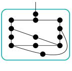
Any signature from is available at a vertex as part of an input graph. Instead of a single vertex, we can use graph fragments to generalize this notion. An -gate is a pair , where is a graph with some dangling edges (Figure 1 contains some examples). Other than these dangling edges, an -gate is the same as a signature grid. The role of dangling edges is similar to that of external nodes in Valiant’s notion [Valiant:Qciricuit], however we allow more than one dangling edge for a node. In each node is assigned a function in (we do not consider “dangling” leaf nodes at the end of a dangling edge among these), are the regular edges, and are the dangling edges. Then we can define a function for this -gate ,
where , , denotes an assignment on the dangling edges, and denotes the value of the partial signature grid on an assignment of all edges, i.e., the product of evaluations at every vertex of , for .


We will also call this function the signature of the -gate . An -gate can be used in a signature grid as if it is just a single node with the same signature. We note that even for a very simple signature set , the signatures for all -gates can be quite complicated and expressive. Matchgate signatures are an example [Valiant:Qciricuit].
The dangling edges of an -gate are considered as input or output variables. Any -input -output -gate can be viewed as a by matrix which transforms arity- signatures into arity- signatures (this is true even if or are 0). Our construction will transform symmetric signatures to symmetric signatures. This implies that there exists an equivalent by matrix which operates directly on column vectors written in symmetric signature notation. We will henceforth identify the matrix with the -gate itself. The constructions in this paper are based upon three different types of bipartite -gates which we call starter gadgets, recursive gadgets, and finisher gadgets. An arity- starter gadget is an -gate with no input but output edges. If an -gate has input and output edges then it is called an arity- recursive gadget. Finally, an -gate is an arity- finisher gadget if it has input edges 1 output edge. As a matter of convention, we consider any dangling edge incident with a generator as an output edge and any dangling edge incident with a recognizer as an input edge; see Figure 1.
3. Interpolation Techniques
3.1. Binary recursive construction
In this section, we develop our new technique of higher dimensional iterations for interpolation of unary signatures.
Lemma 3.1.
Suppose is a nonsingular matrix, is a nonzero vector, and for all integers , is not a column eigenvector of . Let be three matrices, where for , and the intersection of the row spaces of is trivial . Then for every , there exists some , and some , such that and vectors in are pairwise linearly independent.
Proof 3.2.
Let be integers. Then and are nonzero and also linearly independent, since otherwise is an eigenvector of . Let , then , and is a 1-dimensional linear subspace. It follows that there exists an such that the row space of does not contain , and hence has trivial intersection with . In other words, . We conclude that has rank 2, and and are linearly independent.
Each , where , defines a coloring of the set as follows: color with the linear subspace spanned by . Thus, defines an equivalence relation where iff they receive the same color. Assume for a contradiction that for each , where , there are not pairwise linearly independent vectors among . Then, including possibly the 0-dimensional space , there can be at most distinct colors assigned by . By the pigeonhole principle, some and with must receive the same color for all , where . This is a contradiction and we are done. ∎
The next lemma says that under suitable conditions we can construct all unary signatures . The method will be interpolation at a higher dimensional iteration, and finishing up with a suitable finisher gadget. The crucial new technique here is that when iterating at a higher dimension, we can guarantee the existence of one finisher gadget that succeeds on polynomially many steps, which results in overall success. Different finisher gadgets may work for different initial signatures and different input size , but these need not be known in advance and have no impact on the final success of the reduction.
Lemma 3.3.
Suppose that the following gadgets can be built using complex-valued signatures from a finite generator set and a finite recognizer set .
-
(1)
A binary starter gadget with nonzero signature .
-
(2)
A binary recursive gadget with nonsingular recurrence matrix , for which is not a column eigenvector of for any positive integer .
-
(3)
Three binary finisher gadgets with rank 2 matrices , where the intersection of the row spaces of , , and is the zero vector.
Then for any , .