Holographic Dark Energy Models in $f(Q,T)$ Gravity and Cosmic Constraint

Over the past few decades, a series of major discoveries in cosmology have profoundly reshaped our understanding of the universe. In 1998, observations of Type Ia supernova first revealed that the universe is undergoing accelerated expansion [1, 2]. This groundbreaking discovery was later confirmed by various other cosmological observations, including measurements of temperature anisotropies and polarization in the cosmic microwave background (CMB) radiation [3, 4], the peak length scale of baryon acoustic oscillations (BAO) [5, 6], the evolution of the large-scale structure (LSS) of the universe [7, 8], and direct measurements of the Hubble parameter using cosmic chronometers [9, 10]. These observations suggest a mysterious dark energy (DE) with negative pressure, driving this acceleration against gravitational collapse, though its nature remains elusive.

For such accelerated expansion to occur, dark energy must produce a repulsive gravitational effect that permeates the entire observable universe. Ordinary baryonic matter, however, does not exhibit the properties required to explain this phenomenon, nor can it account for such a significant portion of the universe’s energy budget. As a result, researchers have proposed and studied a variety of alternative theories and models to explore the nature of dark energy and the cosmic acceleration it causes [11].

The simplest and most widely accepted theory is $\Lambda\text{CDM}$ model, where $\Lambda$ denotes cosmological constant introduced by Einstein [12]. Based on $\Lambda\text{CDM}$ model, the latest observations suggest that our universe consists of 68.3% dark energy, 26.8% cold dark matter and 4.9% ordinary matter [4]. However, it faces challenges: the fine-tuning problem (why $\Lambda$ is so small), the cosmic coincidence issue (why dark energy dominates now), and the Hubble tension-a discrepancy between the CMB-derived $H_{0}=67.4\pm 0.5\text{km/s/Mpc}$ by Planck [4] and local SNIa-based $73.04\pm 1.04\text{km/s/Mpc}$ [13].

An alternative approach modifies general relativity at large scales, with progress reviewed in [14]. These theories assume that general relativity not works in large scale requiring a modification in action rather than standard Einstein-Hilbert action. The most well-known is $f(R)$ gravity which replaces the Ricci scalar $R$ in the action by a general function $f(R)$ [15]. The $f(G)$ gravity theory is also a modified theory of gravity that introduces a correction to the Gauss–Bonnet (GB) term $G$, allowing it to be arbitrary function $f(G)$ rather than remaining a constant [16, 17]. Another modified theory of gravity $f(T)$ extends the teleparallel equivalent of General Relativity (TEGR). It replaces the curvature scalar $R$ in action with the torsion scalar $T$, derived from the Weitzenböck connection. Also shows some interpretations for the accelerating phases of our Universe [18, 19]. $f(Q)$ is generalized symmetric teleparallel gravity, with curvature and torsion both being zero, which is inspired by Weyl and Einstein’s trial to unify electromagenetic and gravity. The geometric properties of gravity are described by ”non-metricity”. That is, the covariant derivative of the metric tensor is no longer zero (some detailed information can be found in review [20]). Harko et al. have proposed a new theory known as $f(R,T)$ gravity, where $R$ stands for the Ricci scalar and $T$ denotes the trace of energy-momentum tensor which presents a non-minimal coupling between geometry and matter [21]. Similar theories are introduced,$f(R,G)$ gravity proposed by Bamba et al. [22]; $f(Q,T)$ proposed by Xu et al. [23]; $f(Q,C)$ gravity [24]; $f(\mathcal{T},T)$ proposed by [25]; $f(T,B)$ gravity [26, 27]; $f(R,T^{2})$ proposed by Katirci et al. [28], etc.

Holographic dark energy (HDE) is an famous alternative theory for the interpretation of dark energy, originating from the holographic principle proposed by ’t Hooft [29]. Cohen et al. introduced the ”UV-IR” relationship, highlighting that in effective quantum field theory, a system of size $L$ has its entropy and energy constrained by the Bekenstein entropy bound and black hole mass, respectively. This implies that quantum field theory is limited to describing low-energy physics outside black holes [30]. After that, Li et al. proposed that the infrared cut-off relevant to the dark energy is the size of the event horizon and obtained the dark energy density can be described as $\rho_{\text{de}}=3c^{2}M_{p}^{2}R_{h}^{2}$ where $R_{h}$ is future horizon of our universe [31]. Although Hubble cut-off is a natural thought, but Hsu found it might lead to wrong state equation and be strongly disfavored by observational data [32].

Various attempts to reconstruct or discuss HDE in modified gravity have been completed by several authors. Wu and Zhu reconstructed HDE in $f(R)$ gravity [33]. Shaikh et al. discussed HDE in $f(G)$ gravity with Bianchi type 1 model [34]. Zubair et al. reconstructed Tsallis holographic dark energy models in modified $f(T,B)$ gravity [35]. Sharif et al. studied the cosmological evolution of HDE in $f(\mathcal{G},T)$ gravity [36] and Alam et al. investigated Renyi HDE in the same gravity [37]. Myrzakulov et al. reconstructed Barrow HDE in $f(Q,T)$ gravity [38]. Singh et al. and Devi et al. discussed HDE models respectively in $f(R,T)$ gravity and take cosmic constraint [39, 40].

In this article, we assume that our universe is described by $f(Q,T)$ gravity, with HDE as one component of the fluid. In Section 2, we briefly introduce non-Riemannian geometry and $f(Q,T)$ gravity. In Section 3, we incorporate HDE into the model and derive the solution. Section 4 details the observational constraints, followed by results and evolution analysis in Section 5. And Section 6 concludes the findings.

In 1918, Weyl proposed an extension of Riemannian geometry, introducing a non-metricity tensor $Q_{\alpha\mu\nu}=\nabla_{\alpha}g_{\mu\nu}=-w_{\alpha}g_{\mu\nu}$, which describes how the length of a vector changes during parallel transport where $w_{\alpha}$ corresponds to electromagnetic potentials [41].This framework, known as Weyl geometry, can be further extended to Weyl-Cartan geometry by incorporating spacetime torsion [23].

In Weyl-Cartan geometry, the general affine connection is decomposed into three independent components: the Christoffel symbol $\hat{\Gamma}^{\alpha}_{\ \mu\nu}$, the contortion tensor $K^{\alpha}_{\ \mu\nu}$ and the disformation tensor $L^{\alpha}_{\ \mu\nu}$, expressed as [42]:

$$\Gamma^{\alpha}_{\ \mu\nu}=\hat{\Gamma}^{\alpha}_{\ \mu\nu}+K^{\alpha}{}_{\mu\nu}+L^{\alpha}{}_{\mu\nu},$$

(1)

whereas:

	$\displaystyle\hat{\Gamma}^{\alpha}{}_{\mu\nu}$	$\displaystyle=\frac{1}{2}g^{\alpha\beta}(\partial_{\mu}g_{\beta\nu}+\partial_{\nu}g_{\beta\mu}-\partial_{\beta}g_{\mu\nu}),$		(2)
	$\displaystyle K^{\alpha}{}_{\mu\nu}$	$\displaystyle=\frac{1}{2}(T^{\alpha}{}_{\mu\nu}+T_{(\mu}{}^{\alpha}{}_{\nu)})=\frac{1}{2}\left(T^{\alpha}{}_{\mu\nu}+T_{\mu}{}^{\alpha}{}_{\nu}+T_{\nu}{}^{\alpha}{}_{\mu}\right),$		(3)
	$\displaystyle L^{\alpha}{}_{\mu\nu}$	$\displaystyle=\frac{1}{2}(Q^{\alpha}{\mu\nu}-Q_{(\mu}{}^{\alpha}{}_{\nu)})=\frac{1}{2}\left(Q^{\alpha}_{\mu\nu}-Q_{\mu}{}^{\alpha}{}_{\nu}-Q_{\nu}{}^{\alpha}{}_{\mu}\right),$		(4)

are the standard Levi-civita connection of metric $g_{\mu\nu}$, contortion and disformation tensors respectively. In the above definitions, the torsion tensors and the non-metric tensor are introduced as follow:

	$\displaystyle Q_{\rho\mu\nu}$	$\displaystyle\equiv\nabla_{\rho}g_{\mu\nu}=\partial_{\rho}g_{\mu\nu}-\Gamma^{\beta}{}_{\rho\mu}g_{\beta\nu}-\Gamma^{\beta}{}_{\rho\nu}g_{\mu\beta},$		(5)
	$\displaystyle T^{\alpha}{}_{\mu\nu}$	$\displaystyle\equiv 2\Gamma^{\alpha}{}_{[\mu\nu]}=\Gamma^{\alpha}{}_{\mu\nu}-\Gamma^{\alpha}{}_{\nu\mu}.$		(6)

The non-metric tensor has two independent traces, namely $Q_{\mu}=Q_{\mu}{}^{\alpha}{}_{\alpha}$ and $\tilde{Q}^{\mu}=Q_{\alpha}{}^{\mu\alpha}$, which differ by the pair of indices being contracted. so we can get quadratic non-metricity scalar as:

$$Q=\dfrac{1}{4}Q_{\alpha\beta\mu}Q^{\alpha\beta\mu}-\dfrac{1}{2}Q_{\alpha\beta\mu}Q^{\beta\mu\alpha}-\dfrac{1}{4}Q_{\alpha}Q^{\alpha}+\dfrac{1}{2}Q_{\alpha}\tilde{Q}^{\alpha}.$$

(7)

We consider the general form of the Einstein-Hilbert action for the $f(Q,T)$ gravity using units where $8\pi G=1$:

$$S=\int(\frac{1}{2}f(Q,T)+\mathcal{L}_{m})\sqrt{-g}d^{4}x,$$

(8)

where $f$ is an arbitrary function of the non-metricity, $\mathcal{L}_{m}$ is known as matter Lagrangian, $g=\det(g_{\mu\nu})$ denotes determinant of metric tensor, and $T=g^{\mu\nu}T_{\mu\nu}$ is the trace of the matter-energy-momentum tensor, where $T_{\mu\nu}$ is defined as:

$$T_{\mu\nu}=-\frac{2}{\sqrt{-g}}\frac{\delta(\sqrt{-g}\mathcal{L}_{m})}{\delta g^{\mu\nu}}.$$

(9)

Varying the action (8) with respect to the metric tensor $g_{\mu\nu}$ we obtain:

	$\displaystyle\delta S$	$\displaystyle=\int\left(\frac{1}{2}\delta[f(Q,T)\sqrt{-g}]+\delta(\mathcal{L}_{m}\sqrt{-g})\right)d^{4}x$		(10)
		$\displaystyle=\int\frac{1}{2}\left(-\frac{1}{2}fg_{\mu\nu}\sqrt{-g}\delta g^{\mu\nu}+f_{Q}\sqrt{-g}\delta Q+f_{T}\sqrt{-g}\delta T-\frac{1}{2}T_{\mu\nu}\sqrt{-g}\delta g^{\mu\nu}\right)d^{4}x,$		(11)

where $f(Q,T)$ is simplified to $f$, and $f_{Q}=\partial f/\partial Q$, $f_{T}=\partial f/\partial T$. Finally, we obtain the field equation of the $f(Q,T)$ gravity theory:

$$-\frac{2}{\sqrt{-g}}\nabla_{\alpha}(f_{Q}\sqrt{-g}P^{\alpha}_{\ \ \mu\nu})-\frac{1}{2}fg_{\mu\nu}+f_{T}(T_{\mu\nu}+\Theta_{\mu\nu})-f_{Q}(P_{\mu\alpha\beta}Q_{\nu}^{\ \ \alpha\beta}-2Q^{\alpha\beta}_{\ \ \ \ \mu}P_{\alpha\beta\nu})=T_{\mu\nu},$$

(12)

where tensor $\Theta_{\mu\nu}$ are defined as $g^{\alpha\beta}\delta T_{\alpha\beta}/{\delta g^{\mu\nu}}$ and $P^{\alpha}_{\mu\nu}$ is the super-potential of the model (detailed discussion found in [23]). This equation couples non-metricity and matter, extending GR to include geometric and material interactions. When the affine connection vanishes globally (e.g., in the coincidence gauge, where spacetime and tangent space origins align), the non-metricity tensor becomes metric-dependent, recovering Einstein’s GR action.

Assuming that the universe is described by an isotropic, homogeneous and spatially flat Friedmann-Lemaitre-Robertson-Walker (FLRW) spacetime, with the line element expressed as:

$$ds^{2}=-N^{2}(t)dt^{2}+a^{2}(t)\delta_{ij}dx^{i}dx^{j},$$

(13)

where $a(t)$ is the cosmic scale factor used to define the Hubble expansion rate $H=\dot{a}/a$ and the lapse function $N(t)$ used to define dilation rates $\tilde{T}=\dot{N}/N$ (typically set $N(t)=1$ in standard cosmology ). To derive Friedmann equations describing the cosmological evolution, we assume that the matter content of the universe consists of a perfect fluid, whose energy-momentum tensor is given by $T^{\mu}_{\nu}=\text{diag}(-\rho,p,p,p)$ and tensor $\Theta^{\mu}_{\nu}$ is expressed as $\text{diag}(2\rho+p,-p,-p,-p)$. Using the line element (13) and the field equation (12), the modified Friedmann equations in $f(Q,T)$ gravity are:

	$\displaystyle\rho$	$\displaystyle=\frac{f}{2}-6f_{Q}H^{2}-\frac{2f_{T}}{1+f_{T}}(\dot{f}_{Q}H+f_{Q}\dot{H}),$		(14)
	$\displaystyle p$	$\displaystyle=-\frac{f}{2}+6f_{Q}H^{2}+2(\dot{f}_{Q}H+f_{Q}\dot{H}),$		(15)

where $\dot{f}_{Q}=\partial f_{Q}/\partial t$. In the coincident gauge with $\Gamma^{\alpha}_{\mu\nu}=0$, the usage of Eq. (7) and the line element (13), there exists following relationship (The detailed derivation can be found in the appendix of [23] and [43]):

$$Q=6H(t)^{2}.$$

(16)

The equation of state (EoS) parameter is given by

$$w=\frac{p}{\rho}=-1+\frac{4f_{Q}H+f_{Q}\dot{H}}{(1+f_{T})(f-12f_{Q}H^{2})-4f_{T}(\dot{f}_{Q}H+f_{Q}\dot{H})},$$

(17)

where $\rho=\rho_{m}+\rho_{\text{de}}$ and $p=p_{m}+p_{\text{de}}$ represent contributions from baryonic matter and holographic dark energy, respectively, as we focus on the late universe and neglect radiation.

The effective component parameter can be derived from Eq. (14)(15) as:

	$\displaystyle\rho_{\text{eff}}$	$\displaystyle=3H^{2}=\frac{f}{4f_{Q}}-\frac{1}{2f_{Q}}[(1+f_{T})\rho+f_{T}p],$		(18)
	$\displaystyle-p_{\text{eff}}$	$\displaystyle=2\dot{H}+3H^{2}=\frac{f}{4f_{Q}}-\frac{2\dot{f}_{Q}H}{f_{Q}}+\frac{1}{2f_{Q}}[(1+f_{T})\rho+(2+f_{T})p].$		(19)

The two equations describe the total effective energy density $\rho_{\text{eff}}$ and the total effective pressure $p_{\text{eff}}$, reflecting the combined effects of all ideal fluid components and the modified gravity. The term $f/({4f_{Q}})$ represents the contribution from modified gravity, while the latter term accounts for the contributions from various fluid components. However, unlike the standard Friedmann equations, there are correction coefficients $f_{T}$ and $f_{Q}$ that represent interaction modifications. The effective parameters satisfy the conservation equation, but the individual components do not as:

$$\dot{\rho}_{\text{eff}}+3H(\rho_{\text{eff}}+p_{\text{eff}})=0,$$

(20)

though individual components may not conserve due to energy exchange with the modified geometry. Furthermore, the effective EoS using Eq.(18)(19) can be written as:

$$w_{\text{eff}}=\frac{p_{\text{eff}}}{\rho_{\text{eff}}}=\frac{-2\dot{H}-3H^{2}}{3H^{2}}=-\frac{f-8\dot{f}_{Q}H+2[(1+f_{T})\rho+(2+f_{T})p]}{f-2[(1+f_{T})\rho+f_{T}p]},$$

(21)

describing the universe’s overall dynamics, with acceleration occurring when $w_{\text{eff}}<-1/3$.

The holographic principle imposes an upper bound on the entropy of the universe. In the HDE model, the energy density of dark energy is typically expressed as [31]:

$$\rho_{\text{de}}=3c^{2}M_{p}^{2}L^{-2},$$

(22)

where $L$ is the characteristic length scale of the universe, and $c$ is free parameter, and $M_{p}$ is the reduced Planck mass, set to 1 in natural units ($\hbar=c=1$). The Hubble horizon, defined as $L=H^{-1}$, is the simplest choice, though the particle horizon $L_{p}$ and future event horizon $L_{F}$ are also viable alternatives. For the Hubble cutoff, the HDE energy density simplifies to:

$$\rho_{de}=3c^{2}H(t)^{2}$$

(23)

Another HDE model called barrow holographic dark energy (BHDE) generalizes holographic entropy that arises from quantum-gravitational effects which deform the black-hole surface by giving it an intricate, fractal form. Its energy density is given by:

$$\rho_{de}=3c^{2}H(t)^{2-\Delta}$$

(24)

here a new exponent $\Delta$ quantifies the quantum-gravitational deformation, with $\Delta=0$ recovering the standard Bekenstein-Hawking entropy, and $\Delta=1$ corresponding to the most intricate and fractal structure [44].

In order to incorporate HDE in the modified framework, we adopt a simple form of $f$:

$$f(Q,T)=mQ^{n}+\alpha T,$$

(25)

where $Q=6H^{2}$, $T=-\rho+3p$, and $m$, $n$ and $\alpha$ are constants. The partial derivatives are:

$$f_{Q}=mnQ^{n-1}=mn6^{n-1}H^{2n-2},\ f_{T}=\alpha,\ \dot{f}_{Q}=2mn(n-1)6^{n-1}H^{2n-3}\dot{H}.$$

(26)

We also introduce the deceleration factor, which characterizes the acceleration or deceleration of the late universe depending upon its value, defined as:

$$q=\frac{d}{dt}\frac{1}{H}-1=-\frac{\ddot{a}a}{\dot{a}^{2}}=-\frac{\dot{H}}{H^{2}}-1=(1+z)\frac{1}{H(z)}\frac{dH(z)}{dz}-1.$$

(27)

In order to understand the characteristic properties of the dark energy and more easier to get a analytical solution, we need to parameterize EoS of HDE as a constant parameter (it is just like the $w\text{CDM}$ model, and we can also use the CPL parameterization $w_{0}w_{a}\text{CDM}$ [45] which can easily applied with $w_{\text{de}}=w_{0}+w_{a}z/(1+z)$ and we also done it in code):

$$w_{\text{de}}=\frac{p_{\text{de}}}{\rho_{\text{de}}}.$$

(28)

Using Eq.(18) and (19), we derive the energy densities of the dark energy and matter components:

	$\displaystyle\rho_{\text{de}}$	$\displaystyle=\frac{m(2n-1)\left(6H(t)^{2}\right)^{n-1}\left((3\alpha+2)nH^{\prime}(t)+3(\alpha+1)H(t)^{2}\right)}{\left(2\alpha^{2}+3\alpha+1\right)w_{\text{de}}},$		(29)
	$\displaystyle\rho_{m}$	$\displaystyle=\frac{m(2n-1)\left(6H(t)^{2}\right)^{n-1}\left(n(\alpha(w_{\text{de}}-3)-2)H^{\prime}(t)-3(\alpha+1)(w_{\text{de}}+1)H(t)^{2}\right)}{\left(2\alpha^{2}+3\alpha+1\right)w_{\text{de}}}.$		(30)

This is a second order differential equation and it depends on $t$. In order to get cosmological solution, there is also a simple relation between $H(t)$ and $H(z)$:

$$\dot{H}(t)=\frac{d}{dt}H(t)=-\frac{dH(z)}{dz}H(z)(1+z).$$

(31)

Substituting Eq. (24) into Eq.(29) and using the relation (31), we can obtain a differential equation:

$$3c^{2}H(z)^{2-\Delta}=\frac{m6^{n-1}(2n-1)\left(H(z)^{2}\right)^{n-1}\left(3(\alpha+1)H(z)^{2}-(3\alpha+2)n(z+1)H(z)H^{\prime}(z)\right)}{\left(2\alpha^{2}+3\alpha+1\right){w_{\text{de}}}}.$$

(32)

In principle, $H(z)$ can be derived by solving this equation. However, analytical solutions are challenging for higher-order cases. Thus, we first consider $n=1$ and $\Delta=0$ with the initial condition $H(z=0)=H_{0}$ which denotes value of the Hubble parameter at present, yielding:

$$H(z)=H_{0}(1+z)^{\frac{3(1+\alpha)\left(m-c^{2}w_{\text{de}}(1+2\alpha)\right)}{m(2+3\alpha)}}.$$

(33)

We thus obtain the power-law evolution of the Universe which avoids the big-bang singularity similar to the $f(R,T)$ situation in [46]. The corresponding deceleration parameter is:

$$q=-1+\frac{3(\alpha+1)\left(m-(2\alpha+1)c^{2}w_{\text{de}}\right)}{(3\alpha+2)m}.$$

(34)

Here, the deceleration parameter $q$ is a constant that only depends on the model parameters. By choosing specific parameter values, the model can exhibit either accelerated or decelerated expansion. However, since both the deceleration parameter and the effective EoS are time-independent, this model precludes phase transition between accelerated and decelerated expansion phases. To address this limitation and derive a tighter UV cutoff, we use Eq. (24) and set $\Delta=1$, which leads to the following expression for $H(z)$:

$$H(z)=H_{0}(1+z)^{\frac{3(\alpha+1)}{3\alpha+2}}-(1+2\alpha)c^{2}w_{de}\left((1+z)^{\frac{3(\alpha+1)}{3\alpha+2}}-1\right)\frac{1}{m}.$$

(35)

The deceleration parameter becomes:

$$q=\frac{(2\alpha+1)c^{2}w_{\text{de}}\left(3\alpha+(1+z)^{\frac{3(\alpha+1)}{3\alpha+2}}+2\right)-H_{0}m(1+z)^{\frac{3(\alpha+1)}{3\alpha+2}}}{(3\alpha+2)\left((2\alpha+1)c^{2}w_{\text{de}}\left((1+z)^{\frac{3(\alpha+1)}{3\alpha+2}}-1\right)-H_{0}m(1+z)^{\frac{3(\alpha+1)}{3\alpha+2}}\right)}.$$

(36)

And if we set $\Delta=0.5$, we can also get a solution analytically as follow:

$$\begin{split}H(z)&=\left(2\alpha c^{2}w_{\text{de}}+c^{2}w_{\text{de}}\right.\\ &\quad+(1+z)^{\frac{3(\alpha+1)}{6\alpha+4}}\left(2\left((2\alpha+1)^{2}c^{4}H_{0}\right)^{1/2}m^{2}w_{\text{de}}^{2}\right.\\ &\quad\left.\left.+c^{4}(2\alpha w_{\text{de}}+w_{\text{de}})^{2}+H_{0}m^{2}\right)^{1/2}\right)^{2}\frac{1}{m^{2}}\end{split}$$

(37)

In this case, the deceleration factor and effective EOS is also approaching a constant value, similar to the situation of $\Delta=0$. However, in some other situation, if $n\neq 1$ and $\Delta\neq 1\ \text{or}\ 0.5$, higher-order differential equations are difficult to solve analytically, so we can only obtain numerical solutions through complex machine computing. We also consider the case where $\alpha=1$ that reduces it to the minimal matter-energy-momentum tensor coupling.

For comparison in the parameter estimates below, we also consider the case of the standard $\Lambda$CDM model:

$$H(z)=H_{0}\sqrt{\Omega_{m}(1+z)^{3}+\Omega_{\Lambda}},$$

(38)

where $\Omega_{m}=\rho_{m0}/3H_{0}^{2}$ is the matter density parameter, and $\Omega_{\Lambda}=\rho_{\text{de}0}/3H_{0}^{2}$ is the dark energy density parameter. This model assumes that the universe is composed of matter and a cosmological constant $\Lambda$ with no additional exotic components.

In this work, we estimate the cosmological parameters of the model by employing a Markov Chain Monte Carlo (MCMC) method based on the minimization of the chi-square function, $\chi^{2}$ which is given by [51]:

$$\chi^{2}=\sum_{i}\left(\frac{D_{i}-T_{i}(\mathbf{\theta})}{\sigma_{i}}\right)^{2},$$

(39)

where $D_{i}$ represents the $i$-th data point, $T_{i}(\mathbf{\theta})$ is the theoretical prediction for the corresponding quantity, and $\sigma_{i}$ is the error associated with the $i$-th data point. Here, $\mathbf{\theta}$ denotes the vector of model parameters. To complete the parameter constraints, we utilize the Python package emcee¹¹1https://github.com/dfm/emcee [52], a user-friendly MCMC implementation well-suited for cosmological data analysis.

For our analysis, we combine three independent observational datasets:

1. Baryon Acoustic Oscillations (BAO): The BAO measurements provide a standard ruler for distance measurements in the universe. We use the data from the SDSS Baryon Oscillation Spectroscopic Survey (BOSS) [49], Dark Energy Spectroscopic Instrument (DESI) first year data [50] and 6dF Galaxy Survey (6dFGS) to constrain the cosmological parameters [48]. The comoving horizon distance, the transverse comoving distance and the volume-averaged distance combining line-of-sight and transverse distances defined as follow:

	$\displaystyle D_{H}$	$\displaystyle=\frac{c}{H(z)},$		(40)
	$\displaystyle D_{M}$	$\displaystyle=\frac{d_{L}}{1+z},$		(41)
	$\displaystyle D_{V}$	$\displaystyle=\left[\frac{cz}{H(z)}\right]^{1/3}\left[\frac{d_{L}}{1+z}\right]^{2/3},$		(42)

where $d_{L}$ is the luminosity distance (defined in Eq. (45)). When scaled by the sound horizon at the drag epoch $r_{d}$ , ratios such as $D_{H}/r_{d}$, $D_{M}/r_{d}$, and $D_{V}/r_{d}$ serve as important observables for constraining cosmological models and testing the standard model of cosmology.

2. Cosmic chronometers (CC) Measurements: The Hubble parameter measurements, known as the chronometers data, provide independent estimates of the Hubble parameter $H(z)$ at various redshifts. These data serve as an important probe of the expansion rate of the universe. We choose the dataset from [53] which includes 32 CC data points incorporating both the statistical and systematic errors within the redshift range of $0.07<z<1.965$.

3. Type Ia supernova (SNIa) Data: SNIa are considered standard candles because when the light curve reaches its maximum, the absolute luminosity is almost the same. The distance modulus $\mu$ can be obtained according to the following formula:

$$\mu_{obs}=m-M.$$

(43)

On the other hand, we can get the theoretical distance modulus from the cosmological model:

$$\mu_{th}(z)=5\log_{10}d_{L}(z)+25+M_{b},$$

(44)

where $M_{b}$ denotes the absolute luminosity of SNIa and the luminosity distance is defined as:

$$d_{L}(z)=\frac{c}{H_{0}}(1+z)\int_{0}^{z}\frac{dz^{\prime}}{E(z^{\prime})}.$$

(45)

In this paper, we use Pantheon+ dataset who comprises 1701 SNIa samples ²²2https://github.com/PantheonPlusSH0ES/DataRelease, an increase from the 1048 samples in Pantheon dataset and correspond to light curves of 1550 spectroscopically confirmed SNIa within the redshift range $0.001<z<2.26$ [54, 55].

The combined likelihood function $\mathcal{L}$ is then constructed by multiplying the individual likelihoods of each dataset:

$$\mathcal{L}=\mathcal{L}_{\text{BAO}}\times\mathcal{L}_{\text{OHD}}\times\mathcal{L}_{\text{SNIa}},$$

(46)

Thus, the total $\chi^{2}_{\text{tot}}$ is:

$$\chi^{2}_{\text{tot}}=\chi^{2}_{\text{BAO}}+\chi^{2}_{\text{OHD}}+\chi^{2}_{\text{SNIa}}.$$

(47)

To test the statistical significance of our constraints, we implement the Akaike Information Criterion (AIC) and Bayesian Information Criterion (BIC), these criteria may help balance model fit and complexity. the AIC is given by:

$$\text{AIC}=2k-2\ln(\mathcal{L}),$$

(48)

where $k$ is the number of parameters and $\mathcal{L}$ is the likelihood. Similarly, the BIC for each model is calculated as:

$$\text{BIC}=k\ln(n)-2\ln(\mathcal{L}),$$

(49)

where $n$ is the number of data points. Models with lower AIC and BIC values are favored, aiding comparisons between HDE variants and $\Lambda$CDM.

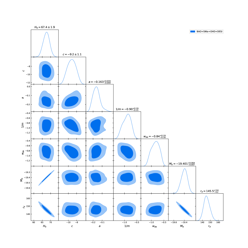
In this research, we use python package GetDist³³3https://github.com/cmbant/getdist [56] from chains of results to plot the corner figure as shown in Fig. 1. The results of the parameter constraints obtained in our analysis are summarized in Table 2. And the best fitting results of the models are also shown in Fig. 3 and Fig. 4. Here we choose the best fitting model maximal deformation $f(Q,T)$ HDE with $\Delta=1$, that we find the following 95% confidence limits for the cosmological and model parameters: the Hubble constant is $H_{0}=67.4^{+3.6}_{-3.7}\,\text{km/s/Mpc}$, which is consistent with recent Planck measurements, though slightly lower. The parameter $c$, which characterizes the evolution of dark energy, is constrained to $c=-9.2^{+2.0}_{-1.9}$. The parameter $a$, which governs the coupling strength between the energy-momentum tensor and geometry, is found to be $a=-0.163^{+0.082}_{-0.076}$, indicating that there is a small coupling coefficient between the geometric structure and the fluid term and gravitational correction of the interaction is meaningful. The inverse of the coefficient $1/m$ that reflects the degree of modification of gravity is constrained to $1/m=-0.90^{+0.30}_{-0.33}$, reflecting the sensitivity of the model to non-metric geometry, the result shows a tiny and negligible deviation to standard condition. The EOS parameter for dark energy, $w_{\text{de}}$, is constrained to $w_{\text{de}}=-1.01^{+0.38}_{-0.40}$, indicating that dark energy is close to but slightly less than the value for a cosmological constant. The absolute magnitude of the reference galaxy, $M_{b}$, is $M_{b}=-19.40^{+0.11}_{-0.12}$, with a narrow error range consistent with the expected value for the sample of galaxies considered. Finally, the sound horizon at the drag epoch $r_{d}$ is measured to be $r_{d}=145.5^{+8.0}_{-7.5}\,\text{Mpc}$, in agreement with current BAO measurements.

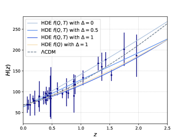
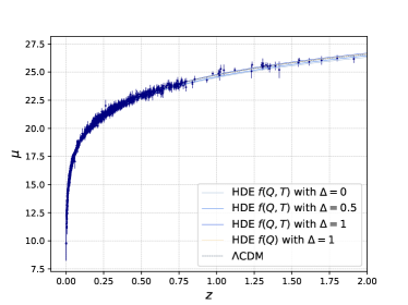
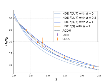
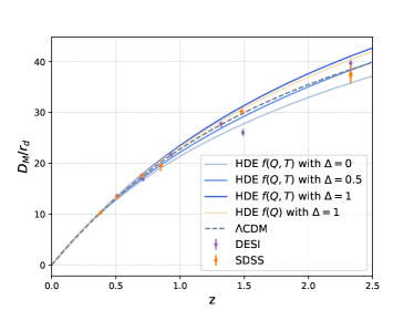
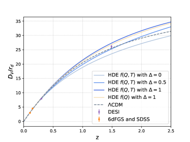
We first plotted the evolution of the Hubble parameter as a function of redshift under the best-fit scenarios for our 4 different models in Fig. 2(a). For comparison, we also included the evolution curve of the $\Lambda$CDM model under the same conditions. We find that the larger $\Delta$ parameter presents a better fit and gradually reduces the value of the Hubble parameter at high redshifts. We also observe that there is a divergence in whether to consider non-minimal coupling, with minimal coupling models that ignore the interaction tending to present a flatter curve. This phenomenon suggests that the interaction in the non-minimal coupling model redistributes the energy between matter and dark energy, thereby reducing the dominance of matter at high redshift. We also plotted the relationship between the supernova distance modulus predicted by the model and the redshift (Fig. 2(b)), along with the data points and error lines obtained from the Pantheon+ dataset, and we found that none of the models were significantly different from the fit of the observed supernova distance modulus. The corresponding best fit curve for BAO data with the data points and error lines are also plotted in Fig. 3.

We can evaluate the model by calculating the AIC and BIC as shown in Table3. However, it is to be expected that these models deviate significantly from the standard $\Lambda$CDM model. The reasons for the deviation are not only due to the large differences caused by non-metric gravitational forces, but also the coupling effects between geometric tensors and dynamic tensors, which cannot be ignored. More importantly, these models have little cosmological motivation, and it is impossible to restore them to any particular limit case [57]. Nonetheless, the results also show that when $\Delta=1$, the dark energy confinement is better than the results in other cases, and that the non-minimally coupled case performs better than the minimally coupled case.

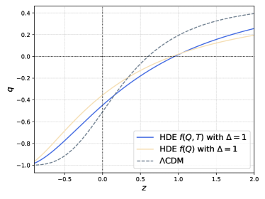
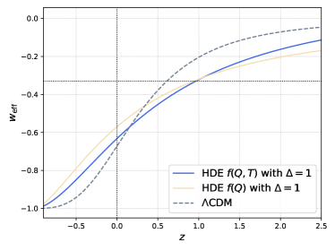
To investigate the evolution of our models, we calculated the deceleration factor and the effective EOS, as shown in Fig. 4(a) and 4(b). Here we plot only two models of the maximum deformation HDE, because for the other two cases, both parameters are approximately constant and cannot reflect the phase transition and accelerated expansion. We find that the evolution of the deceleration factor for the $\Delta=1$ model reveals a transition to an accelerated expansion phase near $z\approx 0.8$ in accordance with relevant observations. At the same time, effective EOS takes into account all the components of the universe, providing a comprehensive reflection of the expansion history of the universe, and in the future this count approaches $-1$, consistent with the cosmological constant dominating the universe, at the current time is also at $w_{\text{eff}}\approx-0.6$ reflecting accelerated expansion phase in our universe.

In this paper, we discuss the evolution of holographic dark energy under the non-metric modified gravity theory $f(Q,T)$. Although this seems to be an overly complex assumption, in fact, if we are in a universe with non-metric geometry (such as Weyl-Cartan geometry) instead of Riemannian geometry, we cannot simply assume that dark energy no longer exists as a fluid in such a universe. We still regard it as one of the reasons for the expansion of the universe, even in such a complex cosmological background.

We also consider holographic dark energy because it has a solid theoretical basis and is a generalization of the holographic principle in cosmology. Holographic dark energy provides a reasonable explanation for the origin of dark energy, namely, it originates from the entanglement entropy of the cosmological horizon. In order to describe holographic dark energy more accurately, we introduce the generalized Barrow holographic dark energy model, which can better characterize quantum corrections. In terms of the choice of infrared cutoff, we use the Hubble horizon as the infrared cutoff point because it is the most natural and simple choice, although other horizons can also be considered. At the same time, in order to facilitate the calculation of analytical solutions, we considered several special cases, namely the loosest restriction when $\Delta=0$, the largest quantum correction when $\Delta=1$, and an intermediate case when $\Delta=0.5$, and discussed whether there is the influence of non-minimal energy-momentum tensor coupling, which makes the interaction between ideal fluid and geometry possible. However, a previous study based on Big Bang Nucleosynthesis (BBN) reports a much tighter constraint on the Barrow exponent, $\Delta\lesssim 1.4\times 10^{-4}$ which is different from our result [58]. This result is in clear tension with ours and highlights the need for further investigation.

To validate the model, we performed parameter estimation using recent supernova data, BAO data, and direct measurements of the Hubble parameter. By employing the MCMC method, we obtained estimates for the model parameters. Our results show that the model can effectively alleviate the Hubble constant tension. Specifically, we find that the Hubble constant is $67.4^{+1.9}_{-1.9}\,\text{km/s/Mpc}$, consistent with Planck 2018 ($H_{0}=67.4\pm 0.5\,\text{km/s/Mpc}$) within 1$\sigma$, but a deviation about 1 $\sigma$ of latest constraint result of $\Lambda$CDM $69.48^{+0.94}_{-0.94}\,\text{km/s/Mpc}$ through DESI BAO and Planck measurements [59], partially alleviating the Hubble constant crisis. We also study the evolution of the universe under this model and observe that the deceleration factor and the effective EOS parameter indicate accelerated expansion, consistent with current observations.

Among the models we considered, we compared AIC and BIC and found that the best result was obtained when $\Delta=1$, which is the maximum deformation of Bekenstein-Hawking entropy and the more stringent ultraviolet cutoff. We also compared it with the case of minimal coupled ones ($\alpha=0$), suggesting that geometry-matter interactions enhance compatibility with observations, despite increased complexity.

Though less compelling due to its numerous parameters and assumptions, this model yields intriguing results and mathematical insights. Its deviations from $\Lambda\text{CDM}$ with non-metric gravity and coupling effects, yet it lacks strong cosmological motivation and specific limiting cases. Nevertheless, this exploration offers potential insights into non-metric gravity’s role in cosmology. Elucidating dark energy’s nature and the universe’s expansion remains an ongoing endeavor, with frameworks like holographical $f(Q,T)$ providing a novel, albeit speculative, perspective.

This work was supported by the National SKA Program of China (Grants Nos. 2022SKA0110200 and 2022SKA0110203). Our code and notebook are available in https://github.com/irosphis/HDE-in-Modified-Gravity.

References

- [1] S. Perlmutter et al. “Discovery of a supernova explosion at half the age of the Universe” In Nature 391.6662, 1998, pp. 51–54 DOI: 10.1038/34124
- [2] Adam G. Riess et al. “Observational Evidence from Supernovae for an Accelerating Universe and a Cosmological Constant” In The Astronomical Journal 116.3 American Astronomical Society, 1998, pp. 1009–1038 DOI: 10.1086/300499
- [3] G.. Smoot et al. “Structure in the COBE Differential Microwave Radiometer First-Year Maps” In apjl 396, 1992, pp. L1 DOI: 10.1086/186504
- [4] N. Aghanim et al. “Planck2018 results: VI. Cosmological parameters” In Astronomy & Astrophysics 641 EDP Sciences, 2020, pp. A6 DOI: 10.1051/0004-6361/201833910
- [5] Daniel J. Eisenstein et al. “Detection of the Baryon Acoustic Peak in the Large‐Scale Correlation Function of SDSS Luminous Red Galaxies” In The Astrophysical Journal 633.2 American Astronomical Society, 2005, pp. 560–574 DOI: 10.1086/466512
- [6] Chris Blake et al. “The WiggleZ Dark Energy Survey: mapping the distance–redshift relation with baryon acoustic oscillations” In Monthly Notices of the Royal Astronomical Society 418.3, 2011, pp. 1707–1724 DOI: 10.1111/j.1365-2966.2011.19592.x
- [7] Scott Dodelson et al. “The Three-dimensional Power Spectrum from Angular Clustering of Galaxies in Early Sloan Digital Sky Survey Data” In The Astrophysical Journal 572.1 American Astronomical Society, 2002, pp. 140–156 DOI: 10.1086/340225
- [8] Will J. Percival et al. “Measuring the Baryon Acoustic Oscillation scale using the Sloan Digital Sky Survey and 2dF Galaxy Redshift Survey: Measuring the BAO scale” In Monthly Notices of the Royal Astronomical Society 381.3 Oxford University Press (OUP), 2007, pp. 1053–1066 DOI: 10.1111/j.1365-2966.2007.12268.x
- [9] Daniel Stern et al. “Cosmic chronometers: constraining the equation of state of dark energy. I: H(z) measurements” In Journal of Cosmology and Astroparticle Physics 2010.02 IOP Publishing, 2010, pp. 008–008 DOI: 10.1088/1475-7516/2010/02/008
- [10] Michele Moresco “Raising the bar: new constraints on the Hubble parameter with cosmic chronometers at z 2” In Monthly Notices of the Royal Astronomical Society: Letters 450.1 Oxford University Press (OUP), 2015, pp. L16–L20 DOI: 10.1093/mnrasl/slv037
- [11] Steven Weinberg “Cosmology” Oxford University Press, 2008 DOI: 10.1093/oso/9780198526827.001.0001
- [12] Sean M. Carroll “The Cosmological Constant” In Living Reviews in Relativity 4.1 Springer ScienceBusiness Media LLC, 2001 DOI: 10.12942/lrr-2001-1
- [13] Adam G. Riess et al. “A Comprehensive Measurement of the Local Value of the Hubble Constant with 1 km s-1 Mpc-1 Uncertainty from the Hubble Space Telescope and the SH0ES Team” In The Astrophysical Journal Letters 934.1 American Astronomical Society, 2022, pp. L7 DOI: 10.3847/2041-8213/ac5c5b
- [14] Timothy Clifton et al. “Modified gravity and cosmology” In Physics Reports 513.1-3 Elsevier BV, 2012, pp. 1–189 DOI: 10.1016/j.physrep.2012.01.001
- [15] H.. Buchdahl “Non-linear Lagrangians and cosmological theory” In MNRAS 150, 1970, pp. 1 DOI: 10.1093/mnras/150.1.1
- [16] Shin’ichi Nojiri et al. “Modified Gauss-Bonnet theory as gravitational alternative for dark energy” In Physics Letters B 631.1, 2005, pp. 1–6 DOI: https://doi.org/10.1016/j.physletb.2005.10.010
- [17] Shin’ichi Nojiri et al. “INTRODUCTION TO MODIFIED GRAVITY AND GRAVITATIONAL ALTERNATIVE FOR DARK ENERGY” In International Journal of Geometric Methods in Modern Physics 04.01 World Scientific Pub Co Pte Ltd, 2007, pp. 115–145 DOI: 10.1142/s0219887807001928
- [18] Yi-Fu Cai et al. “f(T) teleparallel gravity and cosmology” In Reports on Progress in Physics 79.10 IOP Publishing, 2016, pp. 106901 DOI: 10.1088/0034-4885/79/10/106901
- [19] Gabriel R. Bengochea et al. “Dark torsion as the cosmic speed-up” In Physical Review D 79.12 American Physical Society (APS), 2009 DOI: 10.1103/physrevd.79.124019
- [20] Lavinia Heisenberg “Review on f(Q) gravity” Review on f(Q) gravity In Physics Reports 1066, 2024, pp. 1–78 DOI: https://doi.org/10.1016/j.physrep.2024.02.001
- [21] Tiberiu Harko et al. “ gravity” In Phys. Rev. D 84 American Physical Society, 2011, pp. 024020 DOI: 10.1103/PhysRevD.84.024020
- [22] Kazuharu Bamba et al. “Finite-time future singularities in modified Gauss–Bonnet and f(R,G) gravity and singularity avoidance” In The European Physical Journal C 67, 2009, pp. 295–310 URL: https://api.semanticscholar.org/CorpusID:43293585
- [23] Yixin Xu et al. “ gravity” In The European Physical Journal C 79.8 Springer ScienceBusiness Media LLC, 2019 DOI: 10.1140/epjc/s10052-019-7207-4
- [24] Avik De et al. “Non-metricity with boundary terms: gravity and cosmology” In Journal of Cosmology and Astroparticle Physics 2024.03 IOP Publishing, 2024, pp. 050 DOI: 10.1088/1475-7516/2024/03/050
- [25] Tiberiu Harko et al. “ gravity and cosmology” In Journal of Cosmology and Astroparticle Physics 2014.12 IOP Publishing, 2014, pp. 021–021 DOI: 10.1088/1475-7516/2014/12/021
- [26] Sebastian Bahamonde et al. “Modified teleparallel theories of gravity” In Physical Review D 92.10 American Physical Society (APS), 2015 DOI: 10.1103/physrevd.92.104042
- [27] Sebastian Bahamonde et al. “Noether symmetry approach in teleparallel cosmology” In The European Physical Journal C 77.2 Springer ScienceBusiness Media LLC, 2017 DOI: 10.1140/epjc/s10052-017-4677-0
- [28] Nihan Katırcı et al. “ gravity and Cardassian-like expansion as one of its consequences” In The European Physical Journal Plus 129.8 Springer ScienceBusiness Media LLC, 2014 DOI: 10.1140/epjp/i2014-14163-6
- [29] G.’t Hooft “Dimensional Reduction in Quantum Gravity”, 1993 arXiv: https://arxiv.org/abs/gr-qc/9310026
- [30] Andrew G. Cohen et al. “Effective Field Theory, Black Holes, and the Cosmological Constant” Publisher: American Physical Society In Phys. Rev. Lett. 82.25, 1999, pp. 4971–4974 DOI: 10.1103/PhysRevLett.82.4971
- [31] Miao Li “A model of holographic dark energy” In Physics Letters B 603.1, 2004, pp. 1–5 DOI: https://doi.org/10.1016/j.physletb.2004.10.014
- [32] Stephen D.H. Hsu “Entropy bounds and dark energy” In Physics Letters B 594.1-2 Elsevier BV, 2004, pp. 13–16 DOI: 10.1016/j.physletb.2004.05.020
- [33] Xing Wu et al. “Reconstructing theory according to holographic dark energy” In Physics Letters B 660.4, 2008, pp. 293–298 DOI: 10.1016/j.physletb.2007.12.031
- [34] A.Y. Shaikh et al. “Holographic Dark Energy Cosmological Models in f(G) Theory” In New Astronomy 80, 2020, pp. 101420 DOI: 10.1016/j.newast.2020.101420
- [35] M. Zubair et al. “Reconciling Tsallis holographic dark energy models in modified gravitational framework” In The European Physical Journal Plus 136.9, 2021, pp. 943 DOI: 10.1140/epjp/s13360-021-01905-y
- [36] M. Sharif et al. “Cosmic Evolution of Holographic Dark Energy in Gravity” arXiv:1902.05925 [gr-qc, physics:hep-th] arXiv, 2019 URL: http://arxiv.org/abs/1902.05925
- [37] M.. Alam et al. “Renyi Holographic Dark Energy and Its Behaviour in f(G) Gravity” In Astrophysics 66.3, 2023, pp. 383–410 DOI: 10.1007/s10511-023-09798-8
- [38] N. Myrzakulov et al. “Barrow Holographic Dark Energy in f(Q,T) gravity” arXiv:2408.03961 [gr-qc] arXiv, 2024 URL: http://arxiv.org/abs/2408.03961
- [39] C.. Singh et al. “Statefinder diagnosis for holographic dark energy models in modified gravity” In Astrophysics and Space Science 361.5, 2016, pp. 157 DOI: 10.1007/s10509-016-2740-1
- [40] Kanchan Devi et al. “Barrow holographic dark energy model in f(R, T) theory” In Astrophysics and Space Science 369.7, 2024, pp. 73 DOI: 10.1007/s10509-024-04338-y
- [41] H. Weyl “Gravitation and electricity” In Sitzungsber. Preuss. Akad. Wiss. Berlin (Math. Phys. ) 1918, 1918, pp. 465
- [42] Laur Järv et al. “Nonmetricity formulation of general relativity and its scalar-tensor extension” In Physical Review D 97.12 American Physical Society (APS), 2018 DOI: 10.1103/physrevd.97.124025
- [43] Jianbo Lu et al. “Cosmology in symmetric teleparallel gravity and its dynamical system”, 2019 arXiv: https://arxiv.org/abs/1906.08920
- [44] Emmanuel N. Saridakis “Barrow holographic dark energy” In Phys. Rev. D 102 American Physical Society, 2020, pp. 123525 DOI: 10.1103/PhysRevD.102.123525
- [45] MICHEL CHEVALLIER et al. “ACCELERATING UNIVERSES WITH SCALING DARK MATTER” In International Journal of Modern Physics D 10.02 World Scientific Pub Co Pte Lt, 2001, pp. 213–223 DOI: 10.1142/s0218271801000822
- [46] C.. Singh et al. “Statefinder diagnosis for holographic dark energy models in modified gravity” In Astrophysics and Space Science 361.5, 2016, pp. 157 DOI: 10.1007/s10509-016-2740-1
- [47] Orlando Luongo et al. “Dark energy reconstructions combining BAO data with galaxy clusters and intermediate redshift catalogs” arXiv:2411.04901 [astro-ph] arXiv, 2024 DOI: 10.48550/arXiv.2411.04901
- [48] Florian Beutler et al. “The 6dF Galaxy Survey: baryon acoustic oscillations and the local Hubble constant: 6dFGS: BAOs and the local Hubble constant” In Monthly Notices of the Royal Astronomical Society 416.4 Oxford University Press (OUP), 2011, pp. 3017–3032 DOI: 10.1111/j.1365-2966.2011.19250.x
- [49] Shadab Alam et al. “Completed SDSS-IV extended Baryon Oscillation Spectroscopic Survey: Cosmological implications from two decades of spectroscopic surveys at the Apache Point Observatory” In Phys. Rev. D 103 American Physical Society, 2021, pp. 083533 DOI: 10.1103/PhysRevD.103.083533
- [50] DESI Collaboration et al. “DESI 2024 VI: Cosmological Constraints from the Measurements of Baryon Acoustic Oscillations”, 2024 arXiv: https://arxiv.org/abs/2404.03002
- [51] Luis E. Padilla et al. “Cosmological Parameter Inference with Bayesian Statistics” In Universe 7.7 MDPI AG, 2021, pp. 213 DOI: 10.3390/universe7070213
- [52] D. Foreman-Mackey et al. “emcee: The MCMC Hammer” In PASP 125, 2013, pp. 306–312 DOI: 10.1086/670067
- [53] Arianna Favale et al. “Cosmic chronometers to calibrate the ladders and measure the curvature of the Universe. A model-independent study” In Monthly Notices of the Royal Astronomical Society 523.3 Oxford University Press (OUP), 2023, pp. 3406–3422 DOI: 10.1093/mnras/stad1621
- [54] Dan Scolnic et al. “The Pantheon+ Analysis: The Full Data Set and Light-curve Release” In The Astrophysical Journal 938.2 American Astronomical Society, 2022, pp. 113 DOI: 10.3847/1538-4357/ac8b7a
- [55] Dillon Brout et al. “The Pantheon+ Analysis: Cosmological Constraints” In The Astrophysical Journal 938.2 American Astronomical Society, 2022, pp. 110 DOI: 10.3847/1538-4357/ac8e04
- [56] Antony Lewis “GetDist: a Python package for analysing Monte Carlo samples”, 2019 arXiv: https://arxiv.org/abs/1910.13970
- [57] Prabir Rudra et al. “Observational constraint in gravity from the cosmic chronometers and some standard distance measurement parameters” In Nuclear Physics B 967, 2021, pp. 115428 DOI: 10.1016/j.nuclphysb.2021.115428
- [58] John D. Barrow et al. “Big Bang Nucleosynthesis constraints on Barrow entropy” In Physics Letters B 815, 2021, pp. 136134 DOI: https://doi.org/10.1016/j.physletb.2021.136134
- [59] Levon Pogosian et al. “A consistency test of the cosmological model at the epoch of recombination using DESI BAO and Planck measurements”, 2024 arXiv: https://arxiv.org/abs/2405.20306