Holographic Einstein rings of Non-commutative black holes
Abstract
With the help of AdS/CFT correspondence, we derive the desired response function of QFT on the boundary of the non-commutative black hole. Using the virtual optical system with a convex lens, we obtain the Einstein rings of the black hole from the response function. All the results show that the holographic ring always appears with the concentric stripe when the observer located at the north pole. With the change of the observation position, the ring changes into a luminosity-deformed ring, or bright spot. We also investigate the effect of the non-commutative parameter on the ring and find the ring radius becomes larger as the parameter increases. The effect of the temperature on the ring radius is also investigated, it is found that the higher the temperature, the smaller the ring radius. In addition, we also obtain the ingoing angle of the photon via geometric optics, as expected, this angle is consistent well with the angle of the Einstein ring obtained via holography.
I Introduction
In recent years, non-commutative spacetime in gravity theories has become an important research subject Nicolini09 in that it is considered as an alternative way to the quantum gravity Snyder1947 . Many investigations in non-commutative gravity have been done, please see the comprehensive reviews Szabo2006 . In particular, the effects of non-commutativity on black hole physics have attracted much attention, mainly because that the final stage of the noncommutative black hole is more abundant. As is well known, the non-commutativity eliminates point-like structures in favor of smeared objects in flat spacetime Smailagic2006 ; Smailagic2003 and can be implemented in General Relativity by modifying the matter source Nicolini2006 . Therefore, non-commutativity is introduced by modifying mass density so that the Dirac delta function is replaced by a Gaussian distribution Nicolini2006 or alternatively by a Lorentzian distribution Nozari2008 ; Anacleto2020 . In this way the mass density takes the form , where is the noncommutative parameter and is the total mass diffused throughout the region of linear size . With this model in hand, we aim to analyze the lensed effect of a noncommutative black hole in the holographic framework closely followed Hashimoto:2018okj ; Hashimoto:2019jmw .
In the paper Hashimoto:2018okj ; Hashimoto:2019jmw , they proposed a direct procedure to construct holographic images of the black hole in the bulk from a given response function of the QFT on the boundary with the AdS/CFT correspondence. In the holographic picture, the response function with respect to an external source corresponds to the asymptotic data of the bulk field generated by the source on the AdS boundary. For a thermal state on two-dimensional sphere dual to Schwarzschild AdS4 black hole, they demonstrated that the holographic images gravitationally lensed by the black hole can be constructed from the response function. And all these results are consistent with the size of the photon sphere of the black hole calculated by geometrical optics. Closely followed by these breakthroughs, the authors in Liu:2022cev ; Zeng:2023zlf ; Zeng:2023tjb ; Hu:2023eoa ; CEJM ; Hu:2023mai showed that this holographic images do exist in different gravitational backgrounds. However, the photon sphere varies according to the specific bulk dual geometry and the detailed behavior of Einstein ring also varies. Therefore, in this paper, we are tempted to investigate the behavior of the lensed response for the noncommutative black hole and study the effect of the noncommutative parameters on the lensed response.
This paper is arranged as follows. In section II, we briefly review the noncommutative solution in spherically symmeric AdS black hole and introduce the optical system used to observe the Einstein rings. In section III, we first give an explicit constrain on the non-commutative parameter . And then we set up a holographic Einstein ring model and analyze the lensed response function. With the above optical device, we observe the Einstein ring in our model. Section V is the comparison between the holographic method and the geometrical optics method. Our result shows that the position of photon ring obtained from the geometrical optics is full consistence with that of the holographic method. Section VI is devoted to our conclusions.
II Reivew of the holographic construction of Einstein ring in AdS black holes
Gravitational lensing is one of the fundamental phenomena caused by strong gravity. Supposing there is a light source behind a gravitational body, the observers will see a ring-like image of the light source, i.e., the so-called Einstein ring when the light source, the gravitational body, and observers are in alignment. If the gravitational body is a black hole, some light rays are so strongly bended that they can go around the black hole many times, and especially infinite times on the photon sphere. As a result, multiple Einstein rings which correspond to winding numbers of the light ray orbits emerge and infinitely concentrate on the photon sphere. Recently, an observational project for imaging black holes which is called the Event Horizon Telescope (EHT), has captured the first image of the supermassive black hole in M87⋆ and Sagittarius A⋆ EHT ; EventHorizonTelescope:2022wkp . And the dark area inside the photon sphere is named black hole shadow Falcke:1999pj and the shadow of a black hole contains a lot of information. The study of shadow not only enables us to comprehend the geometric structure of spacetime, but also helps us to explore various gravity models more deeply. Following Hashimoto:2018okj ; Hashimoto:2019jmw , the holographic image of an AdS black hole in the bulk was constructed when the wave emitted by the source at the boundary of AdS enters the bulk and then propagates in the bulk by considering the AdS/CFT correspondence Hashimoto:2018okj ; Hashimoto:2019jmw ; Liu:2022cev . Here we first review explicitly the construction of holographic “images” of the dual black hole from the response function of the boundary QFT with external sources.
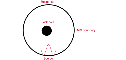
Considering a -dimensional boundary conformal field theory on a 2-sphere at a finite temperature , we study a one-point function of a scalar operator with its conformal dimension , under a time-dependent localized source . The schematic picture of our setup is shown in Fig. 2. For the source , we employ a time-periodic localized Gaussian source with the frequency , amounts to an AdS boundary condition for the scalar field (see Fig. 1). The simplest form of the source is chosen a monochromatic and axisymmetric Gaussian wave packet centered on the south pole . Therefore, the expression of in the ingoing Eddington coordinate is as follows
| (1) | |||||
where is the ingoing Eddington coordinate, represents the width of the wave produced by the Gaussian source and is the spherical harmonics function. We set the wave packet size to be , and the coefficients of the spherical harmonics is
| (2) |
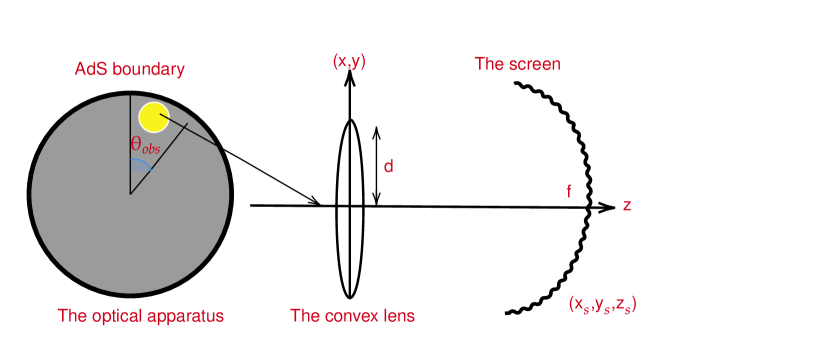
The time-dependent scalar wave propagates inside the black hole spacetime and reaches other points on the of the AdS boundary (please see Fig. 1). Using the optical system shown in Fig. 2, we are able to measure the local response function which contains the information about the bulk geometry of the black hole spacetime Sharma2006 . Explicitly, such optical system consists of a convex lens and a spherical screen. In Fig. 2, the middle position is the lens with focal length regarded as a “converter” between plane and spherical waves and located at . Consider that a plane wave is irradiated to the lens from the left hand side shown in Fig. 2. Such plane wave is converted into spherical wave and converges at the focus . We denote and as the incident wave and the transmitted wave. The conversion between and with frequency on the lens can be mathematically expressed as
| (3) |
We consider a spherical screen located at with . The transmitted wave converted by the lens is focusing and imaging on this screen. The wave function on the screen is given by
| (4) |
where is the distance between on the lens and on the screen. Substituting Eq.(3) into Eq.(4), we have
| (5) |
Using a wave-optical method, we have a formula which helps us convert the response function to the image of the dual black hole on a virtual screen shown as follows
| (6) |
here is Cartesian-like coordinates on boundary and is Cartesian-like coordinates on the virtual screen. Next, we will employ Eq. 6 to obtain the Einstein ring.
III The holographic setup of non-commutative black holes
In this section, we construct the holographic model for the non-commutative Schwarzschild black hole and study the properties of the response function carefully which further helps us to study the Einstein ring. The mass density of a static, spherically symmetric, particle-like gravitational source is no longer a function distribution, but given by a Lorentzian distribution shown as Nicolini2006 ; Nozari2008 ; Anacleto2020
| (7) |
here is the strength of non-commutativity of spacetime and is the total mass diffused throughout a region with linear size . For the smeared matter distribution, we further obtain Anacleto2020
| (8) |
In this case, the non-commutative Schwarzschild black hole metric is given by
| (9) |
with
| (10) |
here is the AdS radius, and we set in the following. According to Eq.(10), we can express the temperature as the inverse of the event horizon
| (11) |
in which . The mass should be non-vanishing, which leads to the following constraint relations
| (12) |
At the event horizon, the corresponding Hawking temperature is
| (13) |
The denominator in Eq.(13) is the same as that in Eq.(11). To assure the temperature is positive, we also should impose the numerator in Eq.(13) is positive, which means
| (14) |
in which
| (15) |
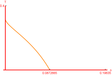
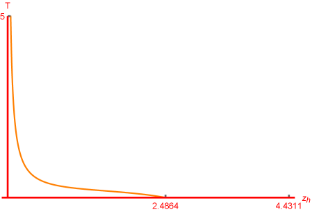
In fact, the constraint in Eq.(14) is much stricter than that in Eq.(12). For a fixed the parameter , from Eq.(14), we know should be smaller than 0.19635, but from Eq.(12), we know should be smaller than 0.0872665, please see Fig. 3, which describes the temperature decreases monotonically as the non-commutative parameter increases. For a fixed , we also can find the relation between and , which is shown in Fig. 4. We find Eq.(14) will produce a constraint while Eq.(12) produces . In Fig. 4, we also see the temperature decreases monotonically as the event horizon increases. These constraints are very important for our later numerical simulation because only parameters that are physically meaningful are important.
We take the complex scalar field as a probe field in the above non-commutative Schwarzschild background. The corresponding dynamics is determined by the Klein-Gordon equation
| (16) |
here is the covariant operator and is a complex scalar field with its mass. And we take in the following.
As before, we prefer the ingoing Eddington coordinate in order to solve the above Eq. (16) in a more convenient way, that is,
| (17) |
here and
| (18) |
Therefore the non-vanishing bulk background fields are transformed into the following smooth form
| (19) |
With , the asymptotic behaviour of near the AdS boundary is expressed as
| (20) |
In the holographic dictionary, is regarded as the source for the boundary field theory. And the response function, which is the corresponding expectation value of the dual operator, is given by
| (21) |
where obviously corresponds to the expectation value of the dual operator with the source turned off.
The bulk solution is easily derived with the source given by Eq. (1)
| (22) |
where satisfies the following equation of motion
| (23) |
and its asymptotic behaviour near the AdS boundary goes
| (24) |
And the resulting response is then written as
| (25) |
with
| (26) |
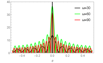
Our main goal is to solve the radial Eq. (23) with the boundary condition at the AdS boundary and vanishes in Eq. (23) at the horizon. With the help of the pseudo-spectral method Liu:2022cev , we obtain the corresponding numerical solution for and . With the extracted , the total response can be obtained by Eq. (25). Here we plot a typical profile of the total response in Fig. 5 to Fig. 7. All the results show that the interference pattern indeed arises from the diffraction of our scalar field by the black hole. Explicitly, Fig. 5 shows the amplitude of for different with and , we can see that the frequency of the Gaussian source increases the width and therefore reduces the wave periods, which means the total response function depends closely on the Gaussian source.
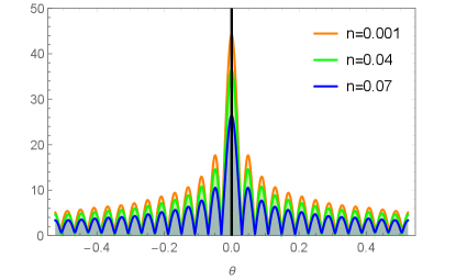
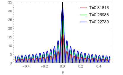
Next we investigate the dependence of the response function on the non-commutative strength parameter . Here we fix the parameters , . From Fig. 6, we see that the amplitude of increases with the decrease of the non-commutativity strength parameter . Similarly, we study the dependence of the total response function on the horizon temperature , which is shown in Fig. 7 with fixed and . The corresponding temperatures are , and . Fig. 7 shows that the amplitude of increases when the temperature decreases.
In all, the total response function depends closely on the Gaussian source and the spacetime geometry. Next, we devoted to convert this response function into an observed images with the optical system described in the section II.
IV Holographic Einstein ring in ADS black hole
According to Eq.(6), we are able to see the observed wave on the screen which is connected with the incident wave by the Fourier transformation. We will set for the source and for the convex lens radius.
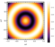
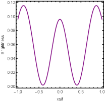


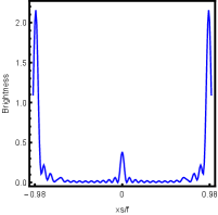
Firstly, we consider the effect of wave source on the characteristics of the holographic Einstein image with different observed from the north pole with the non-commutativity strength parameter and , which is shown in Fig. 8. Here from the left to the right, the values of are , , and , respectively. We can see that the ring is more clear for the high frequency. The corresponding curves which show the brightness of the lensed response on the screen for the same parameters are shown in Fig. 9. The peaks of the curves correspond to the radius of the Einstein ring. From ths figure, we find the higher the frequency becomes, the sharper the Einstein ring becomes. This makes sense because the image can be well captured by the geometric optics approximation in the high frequency limit.
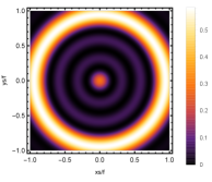
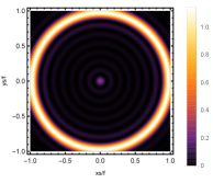
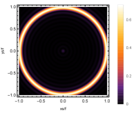
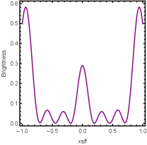
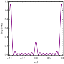
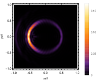
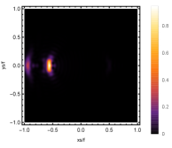
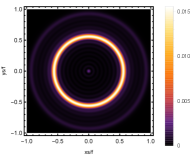
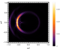
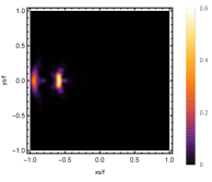
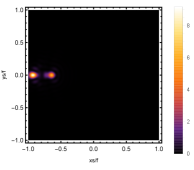
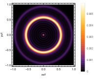
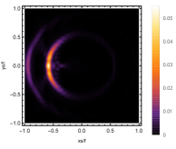
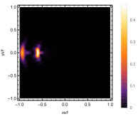
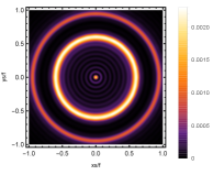
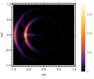
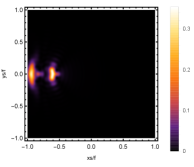
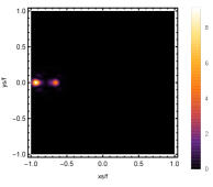
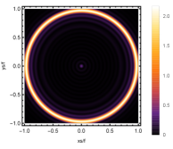
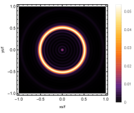
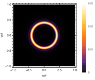
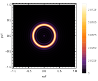
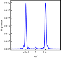
Next, we discuss the influence of different non-commutativity strength parameter on the Einstein ring shown in Fig. 10. Supposing the observer is located at different positions of AdS boundary with the change of the non-commutativity strength parameter for and frequency . When the observer is located at the position , which means the observation is located at the north pole of the AdS boundary. A series of axisymmetric concentric rings appear in the image, and one of them is particularly bright which is shown in the left-most column of Fig. 10. Explicitly from top to bottom, the noncommutativity strength parameter increases from to . And more, as the parameter increases, the brightest ring is away from the center. All these can be clearly seen in Fig. 11 which also shows that the brightness peak of lensed response is far away from the center as the parameter increases for the same parameter. Next we fix the observed position to (the second column from the left shown in Fig. 10). We see the light arcs instead of a strict axisymmetric ring, which are consistent with Zeng:2023tjb ; Zeng:2023zlf . And the positions of the light arcs are away from the center as the parameter increases. That is to say, a series of axisymmetric concentric rings still exist in the image. And from the top to the bottom, we see that the brightness of the ring decreases when the parameter increases. However, when we move to , we see the light arcs become much smaller. When the observer is at , all left are bright spots shown on the right-most column of Fig. 10. And as the parameter increases, the bright spot becomes far away from the center.
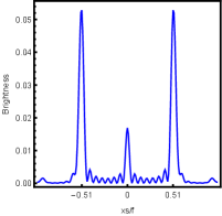
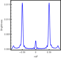
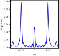
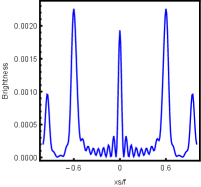
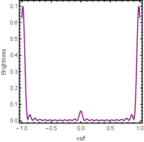
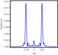
For better understanding the above holographic Einstein image, we also study the impact of the horizon temperature on the lensed response observed with the fixed observation angle . We fix noncommutativity strength parameter and frequency shown in Fig. 12 and the corresponding brightness of the lensed response is in Fig. 13. The four subfigures corresponds to , , and . We find that the brightest ring moves to the center as the temperature increases. This conclusion also can be obtained from Fig. 4, in which the brightness for different temperatures are shown.

V The comparison between the holographic results and optical results
In this section, we compare the results from the holographic dual with the results from the geometrical optics. At the position of the photon sphere, there exists a brightest ring in the image. In this section, we calculate this brightest ring from the viewpoint of optical geometry. In a spacetime with metric in Eq.(9), the ingoing angle of photons from boundary is expressed with the conserved energy and the angular momentum . For generality, we choose the coordinate system in order to let the photon orbit lying on the equatorial plane . The 4-vector satisfies Hashimoto:2018okj ; Zeng:2020vsj
| (27) |
or equivalently,
| (28) |
where , , , and , , .
The ingoing angle with normal vector of boundary should be Hashimoto:2018okj ; Hashimoto:2019jmw
| (29) | |||||
and this implies
| (30) | |||||
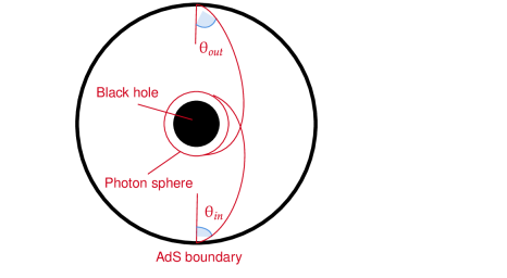
The corresponding ingoing angle of photon orbit from boundary satisfies that
| (31) |
which is shown in Fig. 14. The above relation is still valid when the light is located at the photon sphere. Label the angular momentum as , which is determined by the following conditions
| (32) |
In the geometrical optics, the angle gives the angular distance of the image of the incident ray from the zenith if an observer is located on the AdS boundary looks up into the AdS bulk. When two end points of the geodesic and the center of the black hole are in alignment, the observer sees a ring with a radius corresponding to the incident angle because of axisymmetry Hashimoto:2018okj .
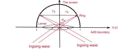
In addition, with Fig. 15, we can obtain the angle of the Einstein ring, which is
| (33) |
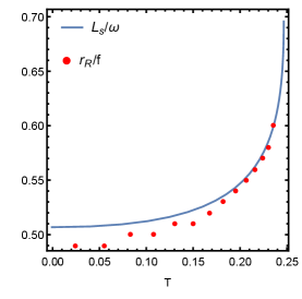
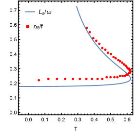
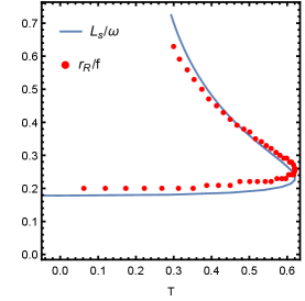
According to Hashimoto:2018okj , for a sufficiently large , we have . Then the desired relation is
| (34) |
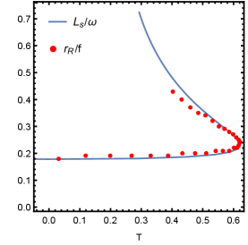
here is the angular momentum at the photon sphere. This relation also can be proved numerically. For different , we find fits well with , which is shown in Fig. 16. Note that for the large , the fitting is more difficult. Even for small , and are not fully the same. In Fig. 17, we discuss the effect of the frequency on the fitting. It is obvious that the larger the frequency, the preciser the fitting.

VI Conclusions
In the framework of AdS/CFT correspondence, we studied the holographic Einstein images of a non-commutative Schwarzschild black hole. We considered a dimensional boundary conformal field theory on a 2-sphere at a finite temperature. Under a time-dependent localized Gaussian source with the frequency , we derived the local response function. Explicitly, the absolute amplitude increases with the decrease of the non-commutative parameter and increases with the decrease of the temperature . We also investigated the effect of the frequency of the wave source on the response function, and found the period decreases as the frequency increases.
With a virtual optical system with a convex lens, we further obtained the Einstein rings. We found the holographic ring always appears with the concentric stripe when the observer located at the north pole while it changes into a luminosity-deformed ring, or bright spot as the observer away from the north pole. The effects of the noncommutative parameter and temperature on the ring were investigated too. It was found that the ring radius becomes larger as the parameter increases, and it becomes smaller as the temperature increases.
To confirm our results, we also investigated the Einstein ring via geometric optics. Especially, we obtained the ingoing angle of the photon. We found that at the Einstein ring, the ingoing angle is the same nearly as that obtained via holography. In addition, we found that frequency affects the fitting accuracy. The higher the frequency, the preciser the result.
Acknowledgements
This work is supported by the National Natural Science Foundation of China (Grants Nos. 11675140, 11705005, 12375043), Innovation and Development Joint Foundation of Chongqing Natural Science Foundation (Grant No. CSTB2022NSCQ-LZX0021) , and Basic Research Project of Science and Technology Committee of Chongqing (Grant No. CSTB2023NSCQ-MSX0324).
References
- (1) P. Nicolini, “Noncommutative Black Holes, The Final Appeal To Quantum Gravity: A Review,” Int. J. Mod. Phys. A 24 (2009), 1229-1308 [arXiv:0807.1939 [hep-th]].
- (2) H. S. Snyder, Phys. Rev. 71 (1947), 38-41.
- (3) R. J. Szabo, “Symmetry, gravity and noncommutativity,” Class. Quant. Grav. 23 (2006), R199-R242 [arXiv:hep-th/0606233 [hep-th]].
- (4) A. Smailagic and E. Spallucci, “Feynman path integral on the noncommutative plane,” J. Phys. A 36 (2003), L467 [arXiv:hep-th/0307217 [hep-th]].
- (5) A. Smailagic and E. Spallucci, “UV divergence free QFT on noncommutative plane,” J. Phys. A 36 (2003), L517-L521 [arXiv:hep-th/0308193 [hep-th]].
- (6) P. Nicolini, A. Smailagic and E. Spallucci, “Noncommutative geometry inspired Schwarzschild black hole,” Phys. Lett. B 632 (2006), 547-551 [arXiv:gr-qc/0510112 [gr-qc]].
- (7) K. Nozari and S. H. Mehdipour, “Hawking Radiation as Quantum Tunneling from Noncommutative Schwarzschild Black Hole,” Class. Quant. Grav. 25 (2008), 175015 [arXiv:0801.4074 [gr-qc]].
- (8) M. A. Anacleto, F. A. Brito, J. A. V. Campos and E. Passos, “Absorption and scattering of a noncommutative black hole,” Phys. Lett. B 803 (2020), 135334 [arXiv:1907.13107 [hep-th]].
- (9) K. Hashimoto, S. Kinoshita and K. Murata, “Imaging black holes through the AdS/CFT correspondence,” Phys. Rev. D 101 (2020) no.6, 066018 [arXiv:1811.12617 [hep-th]].
- (10) K. Hashimoto, S. Kinoshita and K. Murata, “Einstein Rings in Holography,” Phys. Rev. Lett. 123 (2019) no.3, 031602 [arXiv:1906.09113 [hep-th]].
- (11) Y. Liu, Q. Chen, X. X. Zeng, H. Zhang, W. L. Zhang and W. Zhang, “Holographic Einstein ring of a charged AdS black hole,” JHEP 10 (2022), 189 [arXiv:2201.03161 [hep-th]].
- (12) X. X. Zeng, K. J. He, J. Pu, G. p. Li and Q. Q. Jiang, “Holographic Einstein rings of a Gauss–Bonnet AdS black hole,” Eur. Phys. J. C 83 (2023) no.10, 897
- (13) X. X. Zeng, L. F. Li and P. Xu, “Holographic Einstein rings of a black hole with a global monopole,” [arXiv:2307.01973 [hep-th]].
- (14) X. Y. Hu, M. I. Aslam, R. Saleem and X. X. Zeng, “Holographic Einstein Rings of an AdS Black Hole in Massive Gravity,” [arXiv:2308.05132 [gr-qc]].
- (15) X. X. Zeng, M. I. Aslam, R. Saleem and X. Y. Hu, ‘Holographic Einstein Rings of Black Holes in Scalar-Tensor-Vector Gravity,” [arXiv:2311.04680 [gr-qc]].
- (16) X. Y. Hu, X. X. Zeng, L. F. Li and P. Xu, “Holographic study on Einstein ring for a charged black hole in conformal gravity,” [arXiv:2312.13552 [gr-qc]].
- (17) K. Akiyama et al. [Event Horizon Telescope], “First M87 Event Horizon Telescope Results. I. The Shadow of the Supermassive Black Hole,” Astrophys. J. Lett. 875 (2019), L1 [arXiv:1906.11238 [astro-ph.GA]].
- (18) K. Akiyama et al. [Event Horizon Telescope], ‘First Sagittarius A* Event Horizon Telescope Results. I. The Shadow of the Supermassive Black Hole in the Center of the Milky Way,” Astrophys. J. Lett. 930 (2022) no.2, L12 [arXiv:2311.08680 [astro-ph.HE]].
- (19) H. Falcke, F. Melia and E. Agol, “Viewing the shadow of the black hole at the galactic center,” Astrophys. J. Lett. 528 (2000), L13 [arXiv:astro-ph/9912263 [astro-ph]].
- (20) K. Sharma, “Optics: principles and applications,” Academic Press, 2006.
- (21) X. X. Zeng and H. Q. Zhang, “Influence of quintessence dark energy on the shadow of black hole,” Eur. Phys. J. C 80 (2020) no.11, 1058 [arXiv:2007.06333 [gr-qc]].