Holographic Entanglement Negativity for Adjacent Subsystems in
1 Introduction
Quantum entanglement has developed into an ubiquitous feature of modern fundamental physics in recent times connecting a spectrum of diverse areas from condensed matter physics to quantum gravity. In this regard entanglement entropy has evolved as the most significant and convenient measure to characterize the entanglement of a bipartite quantum system in a pure state. From quantum information theory this is defined as the von Neumann entropy of the reduced density matrix of the corresponding subsystem. For -dimensional conformal field theories () the entanglement entropy may be computed through the replica technique developed by Calabrese et al in [1, 2].
In the context of the correspondence, Ryu and Takayanagi in [3, 4] proposed a prescription to compute the entanglement entropy of holographic s. For a subsystem described by a spatial region on the boundary the entanglement entropy is given from this conjecture by the area of the co-dimension two bulk extremal surface anchored on the region . In the recent past this has led to intense research activity into entanglement issues for diverse holographic s both at zero and finite temperatures [5, 6, 7, 8, 9, 10, 11].
Although the entanglement entropy was crucial for the characterization of entanglement for bipartite systems in pure states, it was inadequate as an entanglement measure for mixed quantum states. In a seminal work Vidal and Werner [12] introduced a quantity termed entanglement negativity as a computable measure for the upper bound on the distillable entanglement in mixed states. The non convexity property of this entanglement measure was subsequently established in [13]. Interestingly, the authors in [14, 15, 16] computed this quantity in employing a variant of the usual replica technique involving a certain four point function of the twist/anti-twist fields. This technique has been extensively employed to compute the entanglement negativity of various mixed state configurations in [17, 18, 19, 20, 21, 22].
Naturally, it was critical to establish a holographic description for the entanglement negativity of boundary s in terms of the bulk dual geometry in the scenario. In spite of interesting insights in [23, 24], a clear holographic prescription for the entanglement negativity of s remained an unresolved issue. Two of the present authors (VM and GS) in the articles [25, 26, 27] (CMS) proposed a holographic conjecture for the entanglement negativity of such boundary s which exactly reproduced the [16] results in the large central charge limit.
It is important to emphasize that the CMS conjecture mentioned above refers to the entanglement negativity of a single subsystem within an infinite system described by the boundary . In the articles [15, 16], the authors computed the entanglement negativity of a mixed state characterized by two finite intervals and in a both at zero and finite temperatures. In a recent communication [28], the present authors established an independent holographic conjecture for the entanglement negativity between the two intervals mentioned above in the context of . It was shown there that the corresponding entanglement negativity was characterized by a certain algebraic sum of the geodesic lengths in the bulk space time anchored on the two adjacent intervals, which reduced to the holographic mutual information. Remarkably the holographic entanglement negativity computed from the above prescription exactly reproduced the results both for zero and finite temperatures in the large central charge limit [15, 29]. The holographic conjecture for the entanglement negativity [28] alluded above allowed a direct generalization to the scenario. In this case the entanglement negativity could be characterized in terms of an algebraic sum of the areas of bulk co-dimension two extremal surfaces anchored on the respective subsystems in the boundary . As earlier this reduces to the holographic mutual information between the subsystems.
In this article we provide the first non trivial higher dimensional examples in the context of the correspondence to establish the efficacy of our conjecture. To this end we consider the mixed state of two adjacent subsystems and characterized by rectangular strip geometries and compute the corresponding holographic entanglement negativity in s at both zero and finite temperatures. For zero temperature the bulk configuration is described by the vacuum whereas the finite temperature scenario is described by the -Schwarzschild black hole. For the finite temperature case the computation of the holographic entanglement negativity requires both a low and a high temperature approximations for the areas of the corresponding bulk extremal surfaces. At low temperatures the leading contribution arises from the vacuum corrected by sub leading thermal contributions. Interestingly for the high temperature case on the other hand the thermal contribution are precisely subtracted out. Hence at the leading order the entanglement negativity at high temperature is characterized by the area of the entangling surface on the boundary.
This article is organized as follows, in section we briefly review the computation of the holographic entanglement negativity of two adjacent intervals in the scenario described in [28]. In section we establish the corresponding holographic conjecture for the entanglement negativity of two adjacent subsystems in the context of the correspondence. In the subsequent section we employ our conjecture to compute the holographic entanglement negativity for two adjacent subsystems of rectangular strip geometries at zero temperature from the bulk vacuum. In section we describe the corresponding computation for the finite temperature scenario from a bulk -Schwarzschild black hole. In the final section we summarize our results and present our conclusions and future open issues.
2 Entanglement negativity in
In this section, we briefly recapitulate the essential elements for the entanglement negativity of mixed states in a [14, 15]. To this end we consider a tripartition in the described by the spatial intervals , and with , and represents the rest of the system111Note that the definition of entanglement negativity requires the concept of purification which involves embedding the given bipartite system () in a mixed state, inside a larger system such that the full system is in a pure quantum state. The larger system is then traced out to obtain the required mixed state of the bipartite quantum system. . The reduced density matrix of the subsystem is defined as and is the partial transpose of the reduced density matrix with respect to the interval . The entanglement negativity is defined as the logarithm of the trace norm of the partially transposed reduced density matrix [12], which is expressed as
| (2.1) |
The entanglement negativity may now be obtained through a replica technique as discussed in [14, 15] to determine and the replica limit is given as the analytic continuation of through even sequences to . This leads to the following expression for the entanglement negativity
| (2.2) |
For the mixed state described by the two intervals as shown in Fig. (1), the quantity is given by a four point function of the twist operators on the complex plane from the replica technique described in [14, 15], as follows
| (2.3) |
2.1 Entanglement negativity for two adjacent intervals in vacuum
We first review the computation of the entanglement negativity for the mixed state of two adjacent intervals in a at zero temperature [14, 15] and the corresponding holographic description in [28]. The related configuration may now be obtained by setting with and as shown in Fig. (2) described below.
The quantity in the eq. (2.3) for the two adjacent intervals is now described by a three point function of the twist operators as follows
| (2.4) |
The replica limit on eq. (2.4) now leads to the following expression for the entanglement negativity
| (2.5) |
where is the UV cutoff for the . The ‘const’ term in the above expression may be neglected in the large central charge limit ( see discussion below) [29, 28].
In [28] the present authors demonstrated that the universal part of the three point function in eq.(2.4) is dominant in the large central charge limit and factorizes into two point correlation functions. Employing the geodesic approximation for these two point functions from the standard dictionary then leads us to a holographic conjecture for the entanglement negativity of the configuration described above. In the context of the scenario, the holographic conjecture may be expressed as follows
| (2.6) |
Here is the -dimensional Newton constant and is the geodesic length anchored on the interval . Using the Ryu-Takayanagi conjecture [4, 3] the eq. (2.6) reduces to the following
| (2.7) |
which is precisely the mutual information between the subsystems described by the intervals and . Note that the entanglement negativity is a measure of the upper bound on the distillable entanglement of the bipartite system whereas the mutual information is the upper bound on the total correlations between the subsystems. Therefore they are measures of distinct quantities in quantum information theory. However the universal parts of both are dominant in the large central charge limit and admit a holographic description which match exactly for this particular mixed state configuration 222Note that recently this matching between the universal parts of entanglement negativity and mutual information for the adjacent interval case has also been observed in both local and global quench problems in a [30, 20]. . Note that the full entanglement negativity and the mutual information involve non universal terms which are sub leading in in the holographic ( large central charge) limit as described below.
We would like to emphasize here that the exact relation between the holographic negativity and the holographic mutual information described by eq.(2.7) is valid only for this specific mixed state configuration of adjacent intervals and is not expected to hold for generic mixed states. However it could be shown in [25, 26] that for a bipartite mixed state involving a single interval the holographic entanglement negativity was described by a sum of specific holographic mutual informations between subsystems relevant to the purification. Hence there seems to be a relation between these two measures in the holographic limit whose specific nature depends on the mixed state configuration in question. A quantum information theoretic understanding of this phenomena is an open issue which needs elucidation.
In the scenario being considered here, the bulk dual of the at zero temperature is described by the vacuum, whose metric is given as follows
| (2.8) |
where is the radius of the space time. Employing the conjecture described above [28] the holographic entanglement negativity of the configuration in Fig. (2) may now be obtained as
| (2.9) |
Remarkably the holographic entanglement negativity exactly reproduces the result given in eq. (2.5) in the large central charge limit [29, 28] upon using the Brown-Henneaux formula [31].
Note that here we have utilized the relation from the dictionary that connects the UV cut-off for the boundary to the bulk infra red cut-off () ( to regulate the lengths of geodesics in eq.(2.6) ). The eq.(2.9) suggests that only the leading universal part of the negativity in eq.(2.5) is captured by our conjecture whereas the non-universal constant term is sub leading in the large central charge limit. However the precise renormalization procedure for this is an open issue as the first term in eq.(2.5) depends on the UV cut-off whereas the non-universal part is a constant. We mention here that the same issue also occurs in the Ryu-Takayanagi conjecture for the holographic entanglement entropy of a single interval in a where the non-universal part is once again a constant (see also [32, 33, 34] for related discussions on renormalized entanglement entropy in higher dimensions). In contrast for higher point twist correlators in a relevant to both the entanglement entropy and the entanglement negativity for multiple intervals involve non universal functions ( of the cross ratios). In this case using monodromy techniques it was clearly demonstrated that the universal parts which admit a bulk geometrical description, are dominant in the large central charge limit [35, 36] whereas the non universal functions are sub leading in .
2.2 Entanglement negativity for two adjacent intervals at finite temperature
For the finite temperature case the entanglement negativity for the mixed state described by the configuration in Fig. (2) in the context of may be obtained from eq. (2.4) through the conformal map to the cylinder of circumference . This leads to the following expression for the entanglement negativity
| (2.10) |
where and are the inverse temperature and the UV cut-off in the boundary field theory respectively. As earlier in the large central charge limit the ’const’ term in the above equation may be neglected [29, 28].
The bulk dual for the above case is described by the dimensional Euclidean BTZ black hole whose metric is
| (2.11) |
Here the horizon radius is related to the inverse Hawking temperature as . The holographic entanglement negativity for the two adjacent intervals at a finite temperature may then be obtained from the conjecture eq. (2.6) proposed in [28]. Interestingly as earlier this exactly reproduces the finite temperature result given by eq. (2.10) in the large central charge limit upon using the Brown-Henneaux formula.
3 Holographic entanglement negativity for
In this section we establish the holographic entanglement negativity conjecture for a mixed state described by two adjacent subsystems in a boundary in the context of the scenario which was alluded to in the article [28]. As mentioned in the Introduction this would involve an algebraic sum of the areas of the bulk co-dimension two extremal surfaces anchored on the respective subsystems. From the conjecture described in [28] the holographic entanglement negativity may then be expressed as follows
| (3.1) |
where is the extremal area of the co-dimension two surface anchored on the subsystem . Using the Ryu-Takayanagi prescription [4, 3], it is possible to express the holographic entanglement negativity in the following form
| (3.2) |
where is the holographic entanglement entropy of the subsystem . Interestingly the expression in eq. (3.2) is the holographic mutual information between the two adjacent subsystems modulo a constant factor. We are now ready to employ our holographic conjecture to evaluate the entanglement negativity for two adjacent subsystems described by -dimensional spatial rectangular strip geometries in the boundary which we will describe in the subsequent sections.
4 Holographic entanglement negativity for in vacuum
As mentioned above in this section we now proceed to the computation of the holographic entanglement negativity for two adjacent subsystems described by rectangular strip geometries in the boundary at zero temperature. The corresponding bulk dual geometry in this case is the vacuum space time whose metric in the Poincare coordinates is given as
| (4.1) |
where the radius has been set to . The respective rectangular strip geometries of the two subsystems and depicted in Fig. (3) are then specified as follows
| (4.2) |
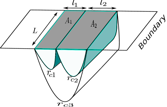
We now briefly describe the computation for the areas of bulk co-dimension two extremal surfaces anchored on rectangular strip geometries in the boundary [4]. The corresponding area functional is expressed in the following way
| (4.3) |
The Euler-Lagrange equation for the extremization problem is then given as
| (4.4) |
where is the turning point of the extremal surface. The extremal area may then be described as
| (4.5) |
where is the UV cutoff and the constant is given as
| (4.6) |
Using the eq.(4.4), eq. (4.5) and eq. (4.6) it is now possible to express the area of the extremal co-dimension two surface as
| (4.7) |
where the divergent part of the area and the constant are given as
| (4.8) | ||||
One may now determine the holographic entanglement negativity for the mixed state at zero temperature in the boundary described by the two strip geometries in Fig. (3) to be as follows
| (4.9) |
The first term in the above expression is the divergent term which is proportional to the area of the entangling surface between the two spatial strips on the dimensional boundary and the second term describes the finite part of the negativity.
5 Holographic entanglement negativity for at finite temperature
At finite temperatures the boundary is dual to the -Schwarzschild black hole with the following metric where the -radius has been set to
| (5.1) |
The horizon radius is related to the Hawking temperature as and are the coordinates on the boundary. We first briefly review the computation for the area of the bulk co-dimension two extremal surface anchored on a single rectangular strip on the boundary as described in [9]. This will be subsequently employed to compute the holographic entanglement negativity for the configuration Fig. (3) in question. The extremal area functional anchored on a single rectangular strip is given as
| (5.2) |
The corresponding Euler-Lagrange equation for the extremization problem leads to the following
| (5.3) |
where as earlier describes the turning point. The area functional in terms of the variable may now be expressed as follows
| (5.4) |
This leads us to the final expression for the area functional as
| (5.5) |
where is the temperature independent divergent part and is the finite part. These may be expressed as follows
| (5.6) | ||||
Note that from [37] ensuring the convergence of the series in . The holographic entanglement negativity for the mixed state described by the two intervals in the boundary ( Fig. (3) ) may then be obtained from our conjecture eq. (3.1) as
| (5.7) |
Here are the turning points of the extremal surfaces in the bulk anchored on the strips and on the boundary respectively. It is required to evaluate the quantity from the eq. (5.3) in terms of and . The corresponding integral is not analytically solvable but may be determined perturbatively for low and high temperature approximations described in the following subsections.
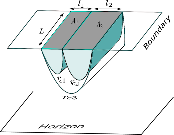
5.1 Holographic entanglement negativity in the low temperature limit
At low temperature we have and may be determined perturbatively as an expansion in [9], which leads to the finite part of the area (5.6) as
| (5.8) |
Here the constants is given by the eq. (4.8) and is given as
| (5.9) |
The holographic entanglement negativity at low temperature for the mixed state in the boundary described by the configuration in Fig (4) may now be obtained from our conjecture (3.1) and the Eqns (5.8) and (5.9) in the following way
| (5.10) | |||||
Here the constant is given as
| (5.11) |
Note that the first and the second term in the above expression are temperature independent describing the contribution to the holographic entanglement negativity from the vacuum eq. (4.9). The remaining terms are the finite temperature corrections to the holographic entanglement negativity at low temperatures for the boundary .
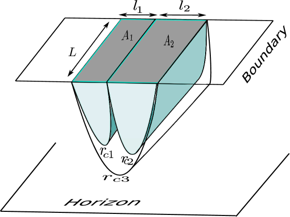
5.2 Holographic entanglement negativity in the high temperature limit
For high temperatures we have and in this case it is possible to obtain the quantity eq. (5.3) in a near horizon expansion in [9] as follows
| (5.12) |
Here is expressed as
| (5.13) | ||||
where the constant is given as
| (5.14) | ||||
The area of the extremal surface at high temperatures is expressed as
| (5.15) | ||||
where and are the volume and area of a single strip respectively . The constant term is given as
| (5.16) | ||||
The holographic entanglement negativity at high temperatures for the mixed state in the boundary described by the configuration in Fig. (5) may then be established from the eq. (5.15) employing our conjecture as follows
| (5.17) | ||||
where the ellipsis represent the higher order corrections and is the area of the entangling surface shared by the two adjacent strips on the boundary. Interestingly in the above expression notice that the thermal contribution to the holographic entanglement negativity (proportional to the volume in the eq. (5.15)) has been subtracted out rendering it to be proportional to the area of the entangling surface. This is in conformity with the usual expectations from quantum information theory and furthermore, recently it has been demonstrated that entanglement negativity does obey an area law in various many body systems such as the finite temperature quantum spin model and the two dimensional harmonic lattice in [38, 39].
6 Summary and conclusions
To summarize we have established a holographic conjecture for the entanglement negativity for mixed states of adjacent subsystems in zero and finite temperature boundary s. The relevant subsystems are described by -dimensional spatial rectangular strip geometries at the boundary in a scenario. Our conjecture involves a certain algebraic sum of the areas of bulk co dimension two extremal surfaces anchored on the corresponding subsystems on the boundary and was motivated by the corresponding analysis for the scenario in [28]. It is interesting that the algebraic sum described above actually characterizes the holographic mutual information between the two adjacent subsystems. Note that these two measures are completely distinct quantities in quantum information theory. Our conjecture states that only their universal parts (which are dominant in the holographic limit) match upto a numerical factor for the particular mixed state configuration of adjacent subsystems. We emphasize that such a matching between the universal parts of negativity and mutual information of adjacent intervals in a has also been demonstrated for both local and global quench problems in [30, 20].
The holographic entanglement negativity for the boundary at zero temperature could then be computed from the bulk dual geometry described by the vacuum from our conjecture. The corresponding holographic entanglement negativity for the boundary at finite temperature however involved a bulk dual geometry described by the -Schwarzschild black hole with a planar horizon. In the latter case the area integrals are not analytically solvable and were evaluated in a perturbative expansion for low and high temperatures. It was observed from our computation that the leading contribution to the holographic entanglement negativity at low temperature arises from the vacuum with subleading thermal corrections. Interestingly on the other hand at high temperatures the finite part of the holographic entanglement negativity is proportional to the area of the entangling surface on the boundary whereas the volume dependent thermal parts cancel out. It has been demonstrated that entanglement negativity does obey such area laws in various condensed matter systems confirming the expectation from quantum information theory (See [38, 39]).
Through these examples we demonstrated that our conjecture provides a direct and elegant holographic prescription to compute the entanglement negativity for mixed states described by the specific configuration in boundary both at zero and finite temperatures. However for the higher dimensional scenario this remains a conjecture. So in higher dimensions our conjecture requires further analysis towards a possible proof from the bulk side which remains a non trivial open issue. In this context our examples serve as a first consistency check in higher dimensions and lead to interesting results described above.
It is well known from quantum information theory that the entanglement negativity characterizes the upper bound on the distillable entanglement for mixed states. It is expected that our conjecture will lead to a deeper understanding of entanglement issues for diverse applications in higher dimensional conformal field theories from condensed matter physics to quantum gravity. It would be interesting to compute the holographic entanglement negativity for subsystems described by more general geometries other than the rectangular strip geometries considered by us. This would possibly lead to deeper insights into the nature of holographic quantum entanglement and its relation to issues of quantum gravity. We expect to return to these exciting issues in the near future.
7 Acknowledgment
Parul Jain would like to thank Prof. Mariano Cadoni for his guidance and the Department of Physics, Indian Institute of Technology Kanpur, India for their warm hospitality. Parul Jain’s work is financially supported by Università di Cagliari, Italy and INFN, Sezione di Cagliari, Italy.
References
- [1] P. Calabrese and J. L. Cardy, “Entanglement entropy and quantum field theory,” J. Stat. Mech. 0406 (2004) P06002, arXiv:hep-th/0405152 [hep-th].
- [2] P. Calabrese and J. Cardy, “Entanglement entropy and conformal field theory,” J. Phys. A42 (2009) 504005, arXiv:0905.4013 [cond-mat.stat-mech].
- [3] S. Ryu and T. Takayanagi, “Holographic derivation of entanglement entropy from AdS/CFT,” Phys. Rev. Lett. 96 (2006) 181602, arXiv:hep-th/0603001 [hep-th].
- [4] S. Ryu and T. Takayanagi, “Aspects of Holographic Entanglement Entropy,” JHEP 08 (2006) 045, arXiv:hep-th/0605073 [hep-th].
- [5] T. Takayanagi, “Entanglement Entropy from a Holographic Viewpoint,” Class. Quant. Grav. 29 (2012) 153001, arXiv:1204.2450 [gr-qc].
- [6] T. Nishioka, S. Ryu, and T. Takayanagi, “Holographic Entanglement Entropy: An Overview,” J. Phys. A42 (2009) 504008, arXiv:0905.0932 [hep-th].
- [7] M. Cadoni and M. Melis, “Entanglement entropy of ads black holes,” Entropy 12 no. 11, (2010) 2244. http://www.mdpi.com/1099-4300/12/11/2244.
- [8] D. D. Blanco, H. Casini, L.-Y. Hung, and R. C. Myers, “Relative entropy and holography,” Journal of High Energy Physics 2013 no. 8, (2013) 60.
- [9] W. Fischler and S. Kundu, “Strongly Coupled Gauge Theories: High and Low Temperature Behavior of Non-local Observables,” JHEP 05 (2013) 098, arXiv:1212.2643 [hep-th].
- [10] W. Fischler, A. Kundu, and S. Kundu, “Holographic Mutual Information at Finite Temperature,” Phys. Rev. D87 no. 12, (2013) 126012, arXiv:1212.4764 [hep-th].
- [11] P. Chaturvedi, V. Malvimat, and G. Sengupta, “Entanglement thermodynamics for charged black holes,” Phys. Rev. D94 no. 6, (2016) 066004, arXiv:1601.00303 [hep-th].
- [12] G. Vidal and R. F. Werner, “Computable measure of entanglement,” Phys. Rev. A 65 (Feb, 2002) 032314. http://link.aps.org/doi/10.1103/PhysRevA.65.032314.
- [13] M. B. Plenio, “Logarithmic Negativity: A Full Entanglement Monotone That is not Convex,” Phys. Rev. Lett. 95 no. 9, (2005) 090503, arXiv:quant-ph/0505071 [quant-ph].
- [14] P. Calabrese, J. Cardy, and E. Tonni, “Entanglement negativity in extended systems: A field theoretical approach,” J. Stat. Mech. 1302 (2013) P02008, arXiv:1210.5359 [cond-mat.stat-mech].
- [15] P. Calabrese, J. Cardy, and E. Tonni, “Entanglement negativity in quantum field theory,” Phys. Rev. Lett. 109 (2012) 130502, arXiv:1206.3092 [cond-mat.stat-mech].
- [16] P. Calabrese, J. Cardy, and E. Tonni, “Finite temperature entanglement negativity in conformal field theory,” J. Phys. A48 no. 1, (2015) 015006, arXiv:1408.3043 [cond-mat.stat-mech].
- [17] P. Calabrese, L. Tagliacozzo, and E. Tonni, “Entanglement negativity in the critical Ising chain,” J. Stat. Mech. 1305 (2013) P05002, arXiv:1302.1113 [cond-mat.stat-mech].
- [18] V. Eisler and Z. Zimboras, “Entanglement negativity in the harmonic chain out of equilibrium,” New Journal of Physics 16 no. 12, (2014) 123020. http://stacks.iop.org/1367-2630/16/i=12/a=123020.
- [19] C.-M. Chung, V. Alba, L. Bonnes, P. Chen, and A. M. Läuchli, “Entanglement negativity via the replica trick: A quantum monte carlo approach,” Phys. Rev. B 90 (Aug, 2014) 064401. https://link.aps.org/doi/10.1103/PhysRevB.90.064401.
- [20] X. Wen, P.-Y. Chang, and S. Ryu, “Entanglement negativity after a local quantum quench in conformal field theories,” Phys. Rev. B92 no. 7, (2015) 075109, arXiv:1501.00568 [cond-mat.stat-mech].
- [21] C. Castelnovo, “Negativity and topological order in the toric code,” Phys. Rev. A 88 (Oct, 2013) 042319. https://link.aps.org/doi/10.1103/PhysRevA.88.042319.
- [22] A. Coser, E. Tonni, and P. Calabrese, “Entanglement negativity after a global quantum quench,” Journal of Statistical Mechanics: Theory and Experiment 2014 no. 12, (2014) P12017. http://stacks.iop.org/1742-5468/2014/i=12/a=P12017.
- [23] V. E. Hubeny, M. Rangamani, and T. Takayanagi, “A Covariant holographic entanglement entropy proposal,” JHEP 07 (2007) 062, arXiv:0705.0016 [hep-th].
- [24] M. Rangamani and M. Rota, “Comments on Entanglement Negativity in Holographic Field Theories,” JHEP 10 (2014) 060, arXiv:1406.6989 [hep-th].
- [25] P. Chaturvedi, V. Malvimat, and G. Sengupta, “Holographic Quantum Entanglement Negativity,” arXiv:1609.06609 [hep-th].
- [26] P. Chaturvedi, V. Malvimat, and G. Sengupta, “Covariant holographic entanglement negativity,” arXiv:1611.00593 [hep-th].
- [27] P. Chaturvedi, V. Malvimat, and G. Sengupta, “Entanglement negativity, Holography and Black holes,” arXiv:1602.01147 [hep-th].
- [28] P. Jain, V. Malvimat, S. Mondal, and G. Sengupta, “Holographic entanglement negativity conjecture for adjacent intervals in ,” arXiv:1707.08293 [hep-th].
- [29] M. Kulaxizi, A. Parnachev, and G. Policastro, “Conformal Blocks and Negativity at Large Central Charge,” JHEP 09 (2014) 010, arXiv:1407.0324 [hep-th].
- [30] A. Coser, E. Tonni, and P. Calabrese, “Entanglement negativity after a global quantum quench,” J. Stat. Mech. 1412 no. 12, (2014) P12017, arXiv:1410.0900 [cond-mat.stat-mech].
- [31] J. D. Brown and M. Henneaux, “Central Charges in the Canonical Realization of Asymptotic Symmetries: An Example from Three-Dimensional Gravity,” Commun. Math. Phys. 104 (1986) 207–226.
- [32] H. Casini and M. Huerta, “Universal terms for the entanglement entropy in 2+1 dimensions,” Nucl. Phys. B764 (2007) 183–201, arXiv:hep-th/0606256 [hep-th].
- [33] H. Liu and M. Mezei, “A Refinement of entanglement entropy and the number of degrees of freedom,” JHEP 04 (2013) 162, arXiv:1202.2070 [hep-th].
- [34] M. Taylor and W. Woodhead, “Renormalized entanglement entropy,” JHEP 08 (2016) 165, arXiv:1604.06808 [hep-th].
- [35] T. Hartman, “Entanglement Entropy at Large Central Charge,” arXiv:1303.6955 [hep-th].
- [36] V. Malvimat and G. Sengupta, “Entanglement negativity at large central charge,” arXiv:1712.02288 [hep-th].
- [37] V. E. Hubeny, “Extremal surfaces as bulk probes in AdS/CFT,” JHEP 07 (2012) 093, arXiv:1203.1044 [hep-th].
- [38] C. De Nobili, A. Coser, and E. Tonni, “Entanglement negativity in a two dimensional harmonic lattice: Area law and corner contributions,” J. Stat. Mech. 1608 no. 8, (2016) 083102, arXiv:1604.02609 [cond-mat.stat-mech].
- [39] N. E. Sherman, T. Devakul, M. B. Hastings, and R. R. P. Singh, “Nonzero-temperature entanglement negativity of quantum spin models: Area law, linked cluster expansions, and sudden death,” Phys. Rev. E 93 (Feb, 2016) 022128. https://link.aps.org/doi/10.1103/PhysRevE.93.022128.