This paper was converted on www.awesomepapers.org from LaTeX by an anonymous user.
Want to know more? Visit the Converter page.

Homoclinic orbits in Kerr-Newman black holes

Yi-Ting Li    Chen-Yu Wang    Da-Shin Lee dslee@gms.ndhu.edu.tw    Chi-Yong Lin lcyong@gms.ndhu.edu.tw Department of Physics, National Dong Hwa University, Hualien, Taiwan, Republic of China
Abstract

We present the exact solutions of the homoclinic orbits for the timelike geodesics of the particle on the general nonequatorial orbits in the Kerr-Newman black holes. The homoclinic orbit is the separatrix between bound and plunging geodesics, a solution that asymptotes to an energetically bound, unstable spherical orbit. The solutions are written in terms of the elliptical integrals and the Jacobi elliptic functions of manifestly real functions of the Mino time where we focus on the effect from the charge of the black hole to the homoclinic orbits. The parameter space of the homoclinic solutions is explored. The nonequatorial homoclinic orbits in Kerr cases can be obtained by setting the charge of the black holes to be zero. The homoclinic orbits and the associated phase portrait as a function of the radial position and its derivation with respect to the Mino time are plotted using the analytical solutions. In particular, the solutions can reduce to the zero azimuthal angular moment homoclinic orbits for understanding the frame dragging effects from the spin as well as the charge of the black hole. The implications of the obtained results to observations are discussed.

pacs:
04.70.-s, 04.70.Bw, 04.80.Cc

I Introduction

Recently successive observations of gravitational waves emitted by the merging of binary systems provide one of the long-awaited confirmations of General Relativity (GR) [1, 2, 3]. The capture of the spectacular images of the supermassive black holes M87* at the center of the M87 galaxy [4] and Sgr A* at the center of our galaxy [5] is also a great achievement that provides direct evidence of the existence of the black holes, the solutions of Einstein’s field equations [6, 7]. Spiraling of stellar mass compact objects into supermassive black holes due to the backreaction of gravitational wave (GW) emission is predicted to be a key source of low frequency gravitational waves, which will be targeted for the planned space-based Laser Interferometer Space Antenna (LISA) [8, 9]. Some of the science goals toward the direct detection of these extreme mass ratio inspirals (EMRIs) are to precisely determine the properties of the EMRIs black hole and its inspiraling components to extract the black hole’s astrophysical environments [10, 11].

The zeroth order approximation in the extreme mass ratio is considered as the small body travels along the geodesic of the background spacetime of the massive black hole. The beginning of the extensive study of the timelike geodesics near the black holes dates back to a remarkable discovery from Carter of the so-called Carter constant [12]. In the family of the Kerr black holes the geodesics of the particle due to the spacetime symmetry of the Kerr family possesses two conserved quantities, the energy EmE_{m} and the azimuthal angular momentum LmL_{m} of the particle. Nevertheless, the existence of the third conserved quantity Carter constant renders the geodesic equations as a set of first-order differential equations. Later, the introduction of the Mino time [13] further fully decouples the geodesics equations with the solutions expressed in terms of the elliptical functions. In this work, we would like to particularly focus on the geodesic dynamics in the case of Kerr-Newman black holes. The Kerr-Newman metric of the solution of the Einstein-Maxwell equations represents a generalization of the Kerr metric, and describes spacetime in the exterior of a rotating charged black hole where, in addition to gravitation fields, both electric and magnetic fields exist intrinsically from the black holes. Although one might not expect that astrophysical black holes have a large residue electric charge, some accretion scenarios were proposed to investigate the possibility of spinning charged back holes [14]. Moreover, theoretical considerations, together with recent observations of structures near Sgr A* by the GRAVITY experiment [15], indicate the possible presence of a small electric charge of central supermassive black hole [16, 17]. Thus, it is still of great interest to explore the geodesic dynamics in the Kerr-Newman black hole.

In our previous paper [18], we have studied the null and timelike geodesics of the light and the neutral particles respectively in the exterior of Kerr-Newman black holes. We classify the roots for both angular and radial potentials, and mainly focus on those of the radial potential with an emphasis on the effect from the charge of the black holes. We then obtain the solutions of the trajectories in terms of the elliptical integrals and the Jacobi elliptic functions for the geodesics, which are manifestly real functions of the Mino time that the initial conditions can be explicitly specified. In this paper, we will mainly focus on the work of [19], which has showed the exact Homoclinic solutions on the equatorial plane in the Kerr black holes, and extend the solutions to a general nonequatorial orbit in the Kerr-Newman black hole with an additional charge. By taking the zero charge limit, the obtained solutions can reduce to those of the nonequatorial homonclinic orbits in the Kerr black holes of more relevance to astrophysical black holes. A homoclinic orbit is the separatrix between bound and plunging geodesics, and is an orbit that asymptotes to an energetically bound, unstable spherical orbit. There are several approaches to model the EMRIs through a series of Kerr geodesics [23, 24, 25, 26, 27, 28, 29, 30, 31, 32]. Due to the dissipation effects from the emission of gravitational radiation on EMRIs, the trajectories of the stellar mass compact object will transit from an inspiral to a plunge through a homoclinic orbit. The exact solutions for the homoclinic orbits could be very useful for analytic or numerical studies of the transition from inspiral to plunge [20, 21]. A thorough knowledge of the underlying dynamics of EMRIs becomes essential to shape the gravitational waveform emitted by them. Also, the added noise provided by the random kicks on the homoclinic orbit will expectedly give the chaotic behavior on the particle moving near the horizon [22]. On top of the fantastic observational effects, it is conjectured that there exists the bound of the Lyapunov exponent based upon the AdS/CFT correspondence [33]. The finding of the exact solution of the homoclinic orbits in the Kerr and Kerr-Newman black holes will be the first step to study the potential chaotic motion when the particle travels near the horizon by explicitly computing the Lyapunov exponents to justify or falsify the conjecture. In this paper, we will start from the analytical solutions of the bound motion derived in [18], and find the solutions of the homoclinic orbits where the particle starts off from the position of the largest root of the radial potential and spent tremendous time moving toward the position of the double root of the radial potential. The parameter space of the homoclinic solutions will also be explored.

In Sec. II, we give a brief review of the timelike geodesic equations from which to define the radial and the angular potentials in terms of the Carter constant CmC_{m} and the azimuthal angular momentum LmL_{m} of the particle normalized by the energy EmE_{m}. The parameter space to have the general nonequatorial homoclinic solutions is explored. Later the results of the homoclinic orbits are adapted from Appendixes which show the solutions of the θ\theta and rr dependence in general bound motion. We then particularly consider the zero azimuthal angular momentum homoclinic orbits, discussing the frame dragging effects in Sec. III. In Sec. IV the phase difference between the nonequatorial homoclinic orbit and the spherical motion of the unstable orbit is considered. In Sec. V the obtained solutions will reduce to the equatorial orbits to compare with [19] in the Kerr black holes as the charge of the black hole in our case is set to zero. All results will be summarized in the closing section.

II Equations of motion for timelike geodesics and Homoclinic orbits

II.1 Equations of motion

We start by reviewing the dynamical equations of the particle in the Kerr-Newman black hole. In the Boyer-Lindquist coordinates the metric for a Kerr-Newman black hole with the gravitational mass MM and spin parameter a=J/Ma=J/M reads as [6]

ds2=ΔΣ(dtasin2θdϕ)2+sin2θΣ[(r2+a2)dϕadt]2+ΣΔdr2+Σdθ2,\displaystyle ds^{2}=-\frac{\Delta}{\Sigma}\left(dt-a\sin^{2}\theta d\phi\right)^{2}+\frac{\sin^{2}\theta}{\Sigma}\left[(r^{2}+a^{2})d\phi-a\,dt\right]^{2}+\frac{\Sigma}{\Delta}dr^{2}+\Sigma d\theta^{2}\;, (1)

where Σ=r2+a2cos2θ\Sigma=r^{2}+a^{2}\cos^{2}\theta and Δ=r22Mr+a2+Q2\Delta=r^{2}-2Mr+a^{2}+Q^{2}. (In this paper we use the geometrized units G=c=1G=c=1.) The outer/inner event horizons r+/rr_{+}/r_{-} are obtained from Δ(r)=0\Delta(r)=0, giving

r±=M±M2(a2+Q2),r_{\pm}=M\pm\sqrt{M^{2}-({a^{2}+Q^{2}})}\;, (2)

which requires M2a2+Q2M^{2}\geq{a^{2}+Q^{2}}.

For the asymptotically flat, stationary and axial-symmetric black holes as in those of (1), the metric is independent of tt and ϕ\phi. The associated Killing vectors can be written as

ξ(t)μ=δtμ,ξϕμ=δϕμ.\displaystyle\xi_{(t)}^{\mu}=\delta_{t}^{\mu},\quad\xi_{\phi}^{\mu}=\delta_{\phi}^{\mu}\,. (3)

The conserved quantities according to the above symmetry, namely the energy EmE_{m} and the azimuthal angular momentum LmL_{m} along a geodesic, can be constructed by the above Killing vectors and the four velocity uμ=dxμ/dσmu^{\mu}=dx^{\mu}/d\sigma_{m} defined in terms of the proper time σm\sigma_{m},

Em\displaystyle E_{m} ξ(t)μuμ,\displaystyle\equiv-\xi_{(t)}^{\mu}u_{\mu}, (4)
Lm\displaystyle L_{m} ξ(ϕ)μuμ.\displaystyle\equiv\xi_{(\phi)}^{\mu}u_{\mu}\,. (5)

The third conservative quantity is the Carter constant written as follows

Cm=Σ2(uθ)2a2Em2cos2θ+Lm2cot2θ+a2m2cos2θ.C_{m}=\Sigma^{2}\left(u^{\theta}\right)^{2}-a^{2}E_{m}^{2}\cos^{2}\theta+L_{m}^{2}\cot^{2}\theta+a^{2}m^{2}\cos^{2}\theta\,. (6)

Together with the timelike geodesics of the particle, uμuμ=m2u^{\mu}u_{\mu}=-m^{2}, the equations of motion for the Boyer-Lindquist coordinates read as

Σdrdσm=±rRm(r),\displaystyle{\Sigma\frac{d{r}}{d\sigma_{m}}}=\pm_{r}\sqrt{R_{m}({r})}\,, (7)
Σdθdσm=±θΘm(θ),\displaystyle{\Sigma\frac{d\theta}{d\sigma_{m}}}=\pm_{\theta}\sqrt{\Theta_{m}(\theta)}\,, (8)
Σdϕdσm=aΔ[(r2+a2)γmaλm]1sin2θ(aγmsin2θλm),\displaystyle{\Sigma\frac{d\phi}{d\sigma_{m}}}=\frac{{a}}{{\Delta}}\left[\left({r}^{2}+{a}^{2}\right)\gamma_{m}-{a}\lambda_{m}\right]-\frac{1}{\sin^{2}\theta}\left({a}\gamma_{m}\sin^{2}\theta-\lambda_{m}\right)\,, (9)
Σdtdσm=r2+a2Δ[(r2+a2)γmaλm]a(aγmsin2θλm),\displaystyle{\Sigma\frac{d{t}}{d\sigma_{m}}}=\frac{{r}^{2}+{a}^{2}}{{\Delta}}\left[\left({r}^{2}+{a}^{2}\right)\gamma_{m}-{a}\lambda_{m}\right]-{a}\left({a}\gamma_{m}\sin^{2}\theta-\lambda_{m}\right)\,, (10)

where

γm=Emm,λmLmm,ηmCmm2.\displaystyle\gamma_{m}=\frac{E_{m}}{m},\hskip 5.69054pt\lambda_{m}\equiv\frac{L_{m}}{m},\hskip 5.69054pt\eta_{m}\equiv\frac{{C}_{m}}{m^{2}}. (11)

The conserved quantities, the energy, the azimuthal angular momentum, and the the Carter constant from (7), (8), (9), and (10) can be determined from the initial conditions. In (7) and (8) the symbols ±r=sign(ur)\pm_{r}={\rm sign}\left(u^{r}\right) and ±θ=sign(uθ)\pm_{\theta}={\rm sign}\left(u^{\theta}\right) are defined by four velocity of the particle. Also in these two equations, the radial and angular potentials Rm(r)R_{m}({r}) and Θm(θ)\Theta_{m}(\theta) are respectively obtained as

Rm(r)=[(r2+a2)γmaλm]2Δ[ηm+(aγmλm)2+r2],\displaystyle R_{m}({r})=\left[\left({r}^{2}+{a}^{2}\right)\gamma_{m}-{a}\lambda_{m}\right]^{2}-{\Delta}\left[\eta_{m}+\left({a}\gamma_{m}-\lambda_{m}\right)^{2}+{r}^{2}\right]\,, (12)
Θm(θ)=ηm+a2γm2cos2θλm2cot2θa2cos2θ.\displaystyle\Theta_{m}(\theta)=\eta_{m}+{a}^{2}\gamma_{m}^{2}\cos^{2}\theta-\lambda_{m}^{2}\cot^{2}\theta-{a}^{2}\cos^{2}\theta\,. (13)

It is known that all equations can be fully decoupled in terms of the so-called Mino time τm\tau_{m} defined as [13]

dxμdτmΣdxμdσm.{\frac{dx^{\mu}}{d\tau_{m}}\equiv\Sigma\frac{dx^{\mu}}{d\sigma_{m}}}\,\,. (14)

For the source point xiμx_{i}^{\mu} and observer point xμx^{\mu}, the integral forms of the equations now becomes [35]

τmτmi\displaystyle\tau_{m}-\tau_{mi} =\displaystyle= Ir=Gθ,\displaystyle{I_{r}}={G_{\theta}}, (15)
ϕϕi\displaystyle{\phi}-{\phi_{i}} =\displaystyle= Iϕ+λmGϕ,\displaystyle{I_{\phi}}+{\lambda_{m}}{G_{\phi}}\,, (16)
tti\displaystyle{t}-{t_{i}} =\displaystyle= It+a2γmGt,\displaystyle{I_{t}}+a^{2}{\gamma_{m}}{G_{t}}\,, (17)

where

Ir\displaystyle I_{r} \displaystyle\equiv rir1±rRm(r)𝑑r,Gθθiθ1±θΘm(θ)𝑑θ,\displaystyle\int_{r_{i}}^{r}\frac{1}{\pm_{r}\sqrt{R_{m}(r)}}dr,\quad G_{\theta}\equiv\int_{\theta_{i}}^{\theta}\frac{1}{\pm_{\theta}\sqrt{\Theta_{m}(\theta)}}d\theta\,, (18)
Iϕ\displaystyle I_{\phi} \displaystyle\equiv rira[(2MrQ2)γmaλm]±rΔRm(r)𝑑r,Gϕθiθcsc2θ±θΘm(θ)𝑑θ,\displaystyle\int_{r_{i}}^{r}\frac{{a\left[\left(2Mr-Q^{2}\right)\gamma_{m}-a\lambda_{m}\right]}}{\pm_{r}\Delta\sqrt{R_{m}(r)}}dr,\quad G_{\phi}\equiv\int_{\theta_{i}}^{\theta}\frac{{\csc^{2}\theta}}{\pm_{\theta}\sqrt{\Theta_{m}(\theta)}}d\theta\,, (19)
It\displaystyle I_{t} \displaystyle\equiv rirr2γmΔ+(2MrQ2)[(r2+a2)γmaλm]±rΔRm(r)𝑑r,Gtθiθcos2θ±θΘm(θ)𝑑θ.\displaystyle\int_{r_{i}}^{r}\frac{{r^{2}\gamma_{m}\Delta+(2Mr-Q^{2})\left[\left(r^{2}+a^{2}\right)\gamma_{m}-a{\lambda_{m}}\right]}}{\pm_{r}\Delta\sqrt{R_{m}(r)}}dr,\;\;G_{t}\equiv\int_{\theta_{i}}^{\theta}\frac{\cos^{2}\theta}{\pm_{\theta}\sqrt{\Theta_{m}(\theta)}}d\theta. (20)

In [18], we have shown the solutions to both null and timelike geodesics. In this work, we will mainly focus on the homoclinic orbits that can be achieved from the alternative expressions of the solutions of the bound motion in [18], which is presented in Appendixes.

Refer to caption
Figure 1: The phase plane of the trajectories. The motions of plunging into the black hole (green), the homoclinic solution (red) as well as the bound motion (purple) in the exterior of the Kerr-Newman black hole (a/M=0.7,Q/M=0.7a/M=0.7,Q/M=0.7).

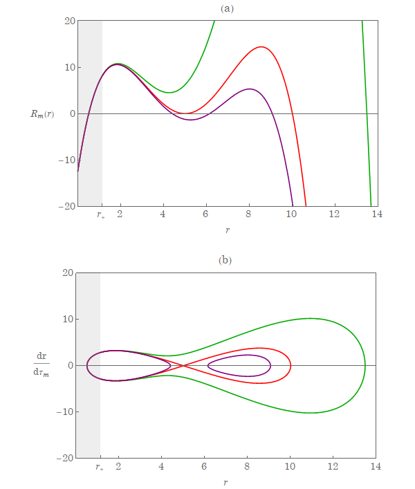
Since the equations of motion are integrable, we thus can construct the diagrams of the exact trajectories on the equatorial plane in terms of rr and dr/dtdr/dt, which reveal qualitative feature of the orbits [22]. In Fig. 1(a) the radial potential Rm(r)R_{m}(r) in (12) is plotted for a few representative parameters of the azimuthal angular momentum λm\lambda_{m} and the Carter constant ηm\eta_{m} for the bound motion (γm<1\gamma_{m}<1). The kinematically allowed regions for the particle to move are for Rm(r)>0R_{m}(r)>0. Three types of motion can be seen from the plot. The green curve is for the case that the particle starts from the largest root of Rm(r)R_{m}(r), moves toward the black hole, and eventually plunges into it. The purple curve is for the particle traveling around the black hole exterior. However, the red curve lies in the separatrix between the two above mentioned motions known as the homoclinic orbit, where the particle starts off from the position of the largest root of the radial potential and spends tremendous time moving toward the position of the double root of the radial potential. The corresponding phase portrait is shown in Fig. 1(b) given by the solutions of (7). All the analytical solutions for such bound motion have been studied in [18]. Here we would like to focus on the analytical solutions of nonequatorial homoclinic orbits and explore the parameter space λm\lambda_{m} and ηm\eta_{m} giving such orbits.

II.2 Homoclinic orbits in the parameter space of λm\lambda_{m} and ηm\eta_{m}

The homoclinic orbits can be characterized by the parameters λm\lambda_{m} and ηm\eta_{m} given by the double root of the radial potential, namely Rm(r)=Rm(r)=0R_{m}\left(r\right)=R_{m}^{\prime}\left(r\right)=0 in (66). They are [18]

λmss=[rmss(MrmssQ2)a2M]γmΔ(rmss)rmss2(γm21)+Mrmssa(rmssM),\displaystyle\lambda_{\rm mss}=\frac{\left[r_{\rm mss}\left(Mr_{\rm mss}-Q^{2}\right)-a^{2}M\right]\gamma_{m}-\Delta\left(r_{\rm mss}\right)\sqrt{r_{\rm mss}^{2}\left(\gamma_{m}^{2}-1\right)+Mr_{\rm mss}}}{a\left(r_{\rm mss}-M\right)}\;, (21)
ηmss=rmssa2(rmssM)2{rmss(MrmssQ2)(a2+Q2Mrmss)γm2.\displaystyle{\eta}_{\rm mss}=\frac{r_{\rm mss}}{a^{2}\left(r_{\rm mss}-M\right)^{2}}\Big{\{}r_{\rm mss}\left(Mr_{\rm mss}-Q^{2}\right)\left(a^{2}+Q^{2}-Mr_{\rm mss}\right)\gamma_{m}^{2}\Big{.}
+2(MrmssQ2)Δ(rmss)γmrmss2(γm21)+Mrmss\displaystyle\quad\quad\quad\quad\quad\quad\quad+2\left(Mr_{\rm mss}-Q^{2}\right)\Delta\left(r_{\rm mss}\right)\gamma_{m}\sqrt{r_{\rm mss}^{2}\left(\gamma_{m}^{2}-1\right)+Mr_{\rm mss}}
.+[a2(MrmssQ2)(Δ(rmss)a2)2][rmss(γm21)+M]},\displaystyle\Big{.}\quad\quad\quad\quad\quad\quad\quad\left.+\left[a^{2}\left(Mr_{\rm mss}-Q^{2}\right)-\left(\Delta\left(r_{\rm mss}\right)-a^{2}\right)^{2}\right]\left[r_{\rm mss}\left(\gamma_{m}^{2}-1\right)+M\right]\Big{\}}\right.\,, (22)

where the subscript “ss” means the spherical orbits with s=±s=\pm, which indicates the two types of motion with respect to the relative sign between the black hole’s spin and the azimuthal angular of the particle (see Sec. III C of [18]).

Refer to caption
Figure 2: The plot shows curves of ISSO (solid line) and IBSO (dashed line) in the parameter space λm\lambda_{m} and ηm\eta_{m}, which demarcate the range of homoclinic solutions (light green). The particle with parameters in the light red and light blue regions plunges into the black hole or scatters by the black hole, respectively. The representative cases are as follows. The parameters of case A can have nonequatorial homoclinic solutions with the zero azimuthal angular momentum orbit where λm=0\lambda_{m}=0, case B for the general nonzero λm\lambda_{m} and ηm\eta_{m}, and case C for equatorial homoclinic orbits with ηm=0\eta_{m}=0 in [19]. The corresponding curves are also shown for Kerr black holes with Q=0Q=0 for comparison.

The spherical orbits with radius rmssr_{\rm mss} coincide with periastron, rmss=rpr_{\rm mss}=r_{p}, which eventually merges with the apastron rar_{a}, the largest root of the radial potential, giving a triple root, also known as innermost stable spherical orbit (ISSO) by decreasing γm\gamma_{m} [18]. On the one hand, solving the triple root equations

Rm(r)=0,Rm(r)=0,Rm′′(r)=0,R_{m}(r)=0\,,\;\;R^{\prime}_{m}(r)=0\,,\;\;R^{\prime\prime}_{m}(r)=0\,, (23)

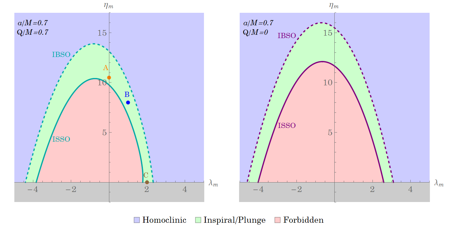
one can demarcate the boundary of ISSO in the parameter space λm\lambda_{m} and ηm\eta_{m}. On the other hand, the bound orbits are limited by the condition γm1\gamma_{m}\to 1 or equivalently rar_{a}\to\infty, known as innermost bound spherical orbit (IBSO). With the double root conditions together with γm=1\gamma_{m}=1, one can find the boundary of IBSO. The parameter region to have homoclinic orbit is bound by the curves ISSO and IBCO in the parameter space λm\lambda_{m} and ηm\eta_{m} as shown in the light green region in Fig. 2. Obviously the particles with the parameters in the light blue (light red) region will evolve unbound (inspiral/plunge) motions. Notice that case A is for the zero azimuthal angular momentum orbit. The frame dragging effect due to the spin of the black hole drives the particle to rotate around the angle ϕ\phi, which will be discussed in Sec. III.

The radii of rissor_{\rm isso}, the triple root of RmR_{m} and ribsor_{\rm ibso}, the radius of the double root together with γm=1\gamma_{m}=1 are given, respectively, by [18]

Mrisso5Δ(risso)+4(Mrisso3Q2risso2+a2ηissoasΓMs)2=0-Mr_{\rm isso}^{5}\Delta\left(r_{\rm isso}\right)+4\left(Mr_{\rm isso}^{3}-Q^{2}r_{\rm isso}^{2}+a^{2}\eta_{\rm isso}-as\sqrt{\Gamma_{\rm Ms}}\right)^{2}=0 (24)

and

Mribso7+(2Mribco3Q2ribso2+a2ηibsoasΓMb)2=0,-Mr_{\rm ibso}^{7}+\left(2Mr_{\rm ibco}^{3}-Q^{2}r_{\rm ibso}^{2}+a^{2}\eta_{\rm ibso}-as\sqrt{\Gamma_{\rm Mb}}\right)^{2}=0\,, (25)

where

ΓMs/b\displaystyle\Gamma_{\rm Ms/b} =risso/ibso4(Mrisso/ibsoQ2)\displaystyle=r_{\rm isso/ibso}^{4}\left(Mr_{\rm isso/ibso}-Q^{2}\right)
ηisso/ibso[risso/ibso(risso/ibso3M)+2Q2]risso/ibso2+a2ηisso/ibso20.\displaystyle-\eta_{\rm isso/ibso}\left[r_{\rm isso/ibso}\left(r_{\rm isso/ibso}-3M\right)+2Q^{2}\right]r_{\rm isso/ibso}^{2}+a^{2}\eta_{\rm isso/ibso}^{2}\geq 0\,. (26)

The radius of the homoclinic orbit lies between the radii rissor_{\rm isso} and ribsor_{\rm ibso} according to the values of λm\lambda_{m} and ηm\eta_{m} of the parameter regions in Fig. 3, in which we have shown the boundaries for various combinations of the black hole parameters aa and QQ.

Refer to caption
Figure 3: The curves ISSO (solid) and IBSO (dashed) in the (λm,ηm)(\lambda_{m},\eta_{m}) parameter space for various combinations of a/Ma/M and Q/MQ/M for Kerr-Newman black holes as well as various choices of a/Ma/M for Kerr black holes with Q=0Q=0. .

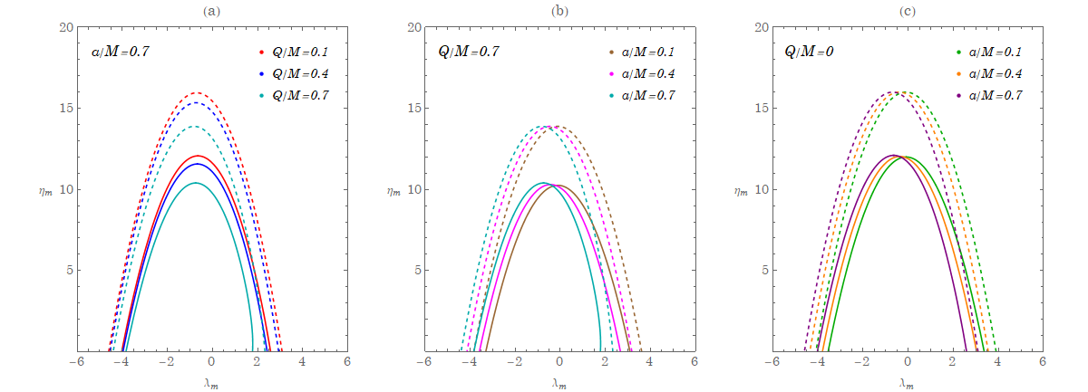
Further detailed explanations for Figs. 2 and 3 have been discussed in [18]. In general, for a fixed value of ηm\eta_{m} and black hole spin aa, since the finite charge of the black hole gives additional repulsive effects to prevent the particle from collapsing into the black hole, the radii of both riscor_{\rm isco} and ribsor_{\rm ibso} will decrease with the increase of the charge, resulting in smaller azimuthal angular momentum |λm||\lambda_{m}|. In addition, for fixed ηm\eta_{m}, the direct orbit will have smaller values of |λm||\lambda_{m}| as compared with the retrograde orbit. Based upon our results, for Sgr A* where the charge is more likely below 101810^{-18} [16, 17], it is not expected to see noticeable difference from the Kerr cases.

II.3 Analytical solutions of homoclinic orbits in general nonequatorial cases

One of the interesting trajectories with the parameters of the double root of the radial potential Rm(r)R_{m}(r) is the homoclinic orbit. In this case, the particle starts from the point of the largest root rm4r_{m4}, moves toward the black hole, and spends an infinity amount of time to reach the point of double roots rm2=rm3=rmssr_{m2}=r_{m3}=r_{\rm mss} with ηmss\eta_{\rm mss} and λmss\lambda_{\rm mss} given by Eqs. (21) and (22). In this case, the analytical expressions summarized in Appendix B gain tremendous simplifications since rm2=rm3r_{m2}=r_{m3} gives the parameter kB=1k^{B}=1, and the elliptical integrals and elliptic functions reduce to elementary functions [36]

F(φ|1)=tanh1(sinφ),\displaystyle F\left(\varphi|1\right)=\tanh^{-1}\left(\sin\varphi\right), (27)
E(φ|1)=sinφ,\displaystyle E\left(\varphi|1\right)=\sin\varphi, (28)
Π(n;φ|1)=1n1[ntanh1(nsinφ)tanh1(sinφ)],\displaystyle\Pi\left(n;\varphi|1\right)=\frac{1}{n-1}\left[\sqrt{n}\tanh^{-1}\left(\sqrt{n}\sin\varphi\right)-\tanh^{-1}\left(\sin\varphi\right)\right], (29)
sn(φ|1)=tanhφ,\displaystyle{\rm sn}\left(\varphi|1\right)=\tanh\varphi, (30)

where π2φπ2,1<n<1-\frac{\pi}{2}\leq\varphi\leq\frac{\pi}{2},\hskip 11.38109pt-1<n<1.

As for the coordinate r(τm)r(\tau_{m}), the homoclinic solution (81) and (82) simplify to the following formulas

rH(τm)=rm4(rm1rmss)rm1(rm4rmss)tanh2(XH(τm))(rm1rmss)(rm4rmss)tanh2XH(τm)r^{H}(\tau_{m})=\frac{r_{m4}(r_{m1}-r_{\rm mss})-r_{m1}(r_{m4}-r_{\rm mss}){{\tanh}^{2}\left(X^{H}(\tau_{m})\right)}}{(r_{m1}-r_{\rm mss})-(r_{m4}-r_{\rm mss}){\tanh}^{2}X^{H}(\tau_{m})} (31)

and

XH(τm)=(1γm2)(rmssrm1)(rm4rmss)2τm.X^{H}(\tau_{m})=\frac{\sqrt{\left(1-\gamma_{m}^{2}\right)({r_{\rm mss}}-r_{m1})(r_{m4}-{r_{\rm mss}})}}{2}\tau_{m}\,. (32)

The other relevant integrals resulting from the radial potentials that contribute to the solutions of the azimuthal angle ϕ(τm)\phi(\tau_{m}) and the time t(τm)t(\tau_{m}) in (16) and (17) are obtained from (84) and (85) giving

Iϕ(τm)=γm1γm22Mar+r[(r+a2MλmγmQ22M)I+H(τm)(ra2MλmγmQ22M)IH(τm)]I_{\phi}(\tau_{m})=\frac{\gamma_{m}}{\sqrt{1-\gamma_{m}^{2}}}\frac{2Ma}{r_{+}-r_{-}}\left[\left(r_{+}-\frac{a}{2M}\frac{\lambda_{m}}{\gamma_{m}}-\frac{Q^{2}}{2M}\right)I_{+}^{H}(\tau_{m})-\left(r_{-}-\frac{a}{2M}\frac{\lambda_{m}}{\gamma_{m}}-\frac{Q^{2}}{2M}\right)I_{-}^{H}(\tau_{m})\right]\quad (33)
It(τm)=γm1γm2{4M2r+r[(r+Q22M)(r+a2MλmγmQ22M)I+H(τm)\displaystyle I_{t}(\tau_{m})=\frac{\gamma_{m}}{\sqrt{1-\gamma_{m}^{2}}}\left\{\frac{4M^{2}}{r_{+}-r_{-}}\left[\left(r_{+}-\frac{Q^{2}}{2M}\right)\left(r_{+}-\frac{a}{2M}\frac{\lambda_{m}}{\gamma_{m}}-\frac{Q^{2}}{2M}\right)I_{+}^{H}(\tau_{m})\right.\right.
(rQ22M)(ra2MλmγmQ22M)IH(τm)]+2MI1H(τm)+I2H(τm)}+(4M2Q2)γmτm\displaystyle\quad\quad\left.\left.-\left(r_{-}-\frac{Q^{2}}{2M}\right)\left(r_{-}-\frac{a}{2M}\frac{\lambda_{m}}{\gamma_{m}}-\frac{Q^{2}}{2M}\right)I_{-}^{H}(\tau_{m})\right]+2MI_{1}^{H}(\tau_{m})+I_{2}^{H}(\tau_{m})\right\}+\left(4M^{2}-Q^{2}\right)\gamma_{m}\tau_{m} (34)

where

I±H(τm)=2(rmssrm1)(rm4rmss){1rm1r±XH(τm)\displaystyle I_{\pm}^{H}(\tau_{m})=\frac{2}{\sqrt{(r_{\rm mss}-r_{m1})(r_{m4}-r_{\rm mss})}}\left\{\frac{1}{r_{m1}-r_{\pm}}X^{H}(\tau_{m})\right.
+rm1rm4(rm1r±)(rm4r±)(h±1)[h±tanh1(xH(τm)h±)tanh1(xH(τm))]}\displaystyle\quad\quad\left.+\frac{r_{m1}-r_{m4}}{(r_{m1}-r_{\pm})\left(r_{m4}-r_{\pm}\right)\left(h_{\pm}-1\right)}\left[\sqrt{h_{\pm}}\tanh^{-1}\left(x^{H}\left(\tau_{m}\right)\sqrt{h_{\pm}}\right)-\tanh^{-1}\left(x^{H}\left(\tau_{m}\right)\right)\right]\right\} (35)
I1H(τm)=2(rmssrm1)(rm4rmss){rm1XH(τm)\displaystyle I_{1}^{H}(\tau_{m})=\frac{2}{\sqrt{(r_{\rm mss}-r_{m1})(r_{m4}-r_{\rm mss})}}\bigg{\{}r_{m1}X^{H}(\tau_{m})
+rm4rm1h1[htanh1(xH(τm)h)tanh1(xH(τm))]}\displaystyle\quad\quad\quad\quad\quad\quad\quad\quad\quad\quad\quad\quad+\frac{r_{m4}-r_{m1}}{h-1}\left[\sqrt{h}\tanh^{-1}\left(x^{H}\left(\tau_{m}\right)\sqrt{h}\right)-\tanh^{-1}\left(x^{H}\left(\tau_{m}\right)\right)\right]\bigg{\}} (36)
I2H(τm)\displaystyle I_{2}^{{H}}(\tau_{m}) =(rH(τm)rm1)(rH(τm)rmss)2(rm4rH(τm))rH(τm)rm1\displaystyle=\frac{\sqrt{\left(r^{H}(\tau_{m})-r_{m1}\right)\left(r^{H}(\tau_{m})-r_{\rm mss}\right)^{2}\left(r_{m4}-r^{H}(\tau_{m})\right)}}{r^{H}(\tau_{m})-r_{m1}}
rmss(rm4rm1)rm1(rm4+rm1)(rmssrm1)(rm4rmss)XH(τm)+(rmssrm1)(rm4rmss)xH(τm)\displaystyle-\frac{r_{\rm mss}\left(r_{m4}-r_{m1}\right)-r_{m1}\left(r_{m4}+r_{m1}\right)}{\sqrt{(r_{\rm mss}-r_{m1})(r_{m4}-r_{\rm mss})}}X^{H}(\tau_{m})+\sqrt{(r_{\rm mss}-r_{m1})(r_{m4}-r_{\rm mss})}x^{H}(\tau_{m})
+(rm4rm1)(rm1+2rmss+rm4)(rmssrm1)(rm4rmss)(h1)[htanh1(xH(τm)h)tanh1(xH(τm))]\displaystyle+\frac{\left(r_{m4}-r_{m1}\right)\left(r_{m1}+2r_{\rm mss}+r_{m4}\right)}{\sqrt{(r_{\rm mss}-r_{m1})(r_{m4}-r_{\rm mss})}(h-1)}\left[\sqrt{h}\tanh^{-1}\left(x^{H}\left(\tau_{m}\right)\sqrt{h}\right)-\tanh^{-1}\left(x^{H}\left(\tau_{m}\right)\right)\right] (37)

In the equations above we have introduced the notations

xH(τm)=(rH(τm)rm4)(rm1rmss)(rH(τm)rm1)(rm4rmss),x^{H}(\tau_{m})=\sqrt{\frac{\left({r^{H}\left(\tau_{m}\right)}-r_{m4}\right)\left(r_{m1}-{r_{\rm mss}}\right)}{\left({r^{H}\left(\tau_{m}\right)}-r_{m1}\right)\left(r_{m4}-{r_{\rm mss}}\right)}}\;, (38)
h±=(rm1r±)(rm4rmss)(rm4r±)(rm1rmss),h=rm4rmssrm1rmss.h_{\pm}=\frac{(r_{m1}-r_{\pm})(r_{m4}-r_{\rm mss})}{(r_{m4}-r_{\pm})(r_{m1}-r_{\rm mss})}\,,\;\;h=\frac{r_{m4}-r_{\rm mss}}{r_{m1}-r_{\rm mss}}\,. (39)

For a given Mino time τm\tau_{m}, the homoclinic orbits along the rr and θ\theta directions can be drawn from the solutions of (60) and (31). Also, the corresponding ϕ\phi and tt can be found through (16) and (17) with the help of Gϕ{G_{\phi}} (61), Iϕ{I_{\phi}} (33), Gt{G_{t}} (63), and It{I_{t}} (34). Together with the solutions along the θ\theta direction, they are the homoclinic solutions for the general nonequatorial orbits in the Kerr-Newman exterior, which are the main results of this work (see Fig. 4). The above expressions can further reduce to the Kerr black hole case by sending Q0Q\rightarrow 0, and also on the equatorial plane [19].

Refer to caption
Figure 4: Illustration of a general nonequatorial homoclinic orbit. The particle with the parameters of case B given in Fig. 2 departs from ri=rm4r_{i}=r_{m4}, the largest root of the radial potential and approaches the unstable spherical orbit rmssr_{\rm mss} of the double root of the radial potential with characteristic angular frequencies shown in the text. The red dotted circle is on the equatorial plane.

III zero azimuthal angular momentum homoclinic orbits

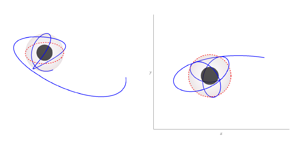
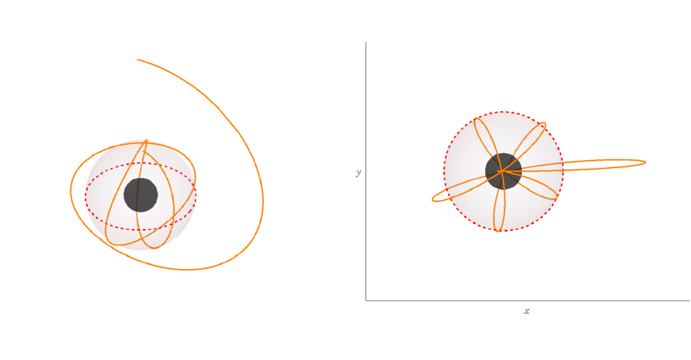
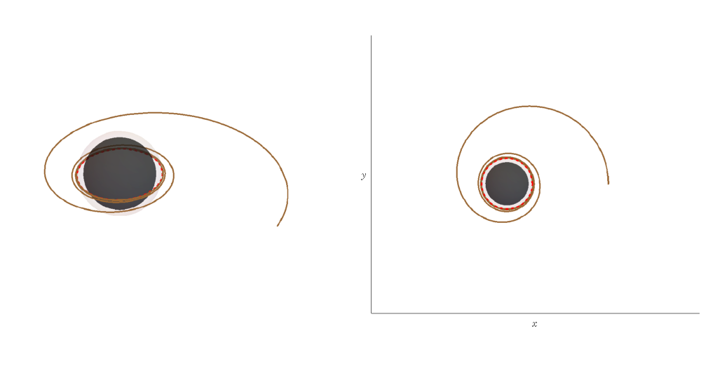
In Sec. II we have shown that the Kerr-Newman spacetimes permit homoclinic orbits in a limited region of parameter space λm\lambda_{m} and ηm\eta_{m}. In particular, a particle with zero azimuthal angular momentum, λmA=0\lambda^{A}_{m}=0, but ηmisso<ηmA<ηmibso\eta_{m}^{\rm isso}<\eta^{A}_{m}<\eta_{m}^{\rm ibso}, can realize homoclinic motion. Using the exact solutions discussed in Sec. II we show in Figs. 5 and 6 two illustrations for this type of motion. The particles share the same set of parameters λm\lambda_{m} and ηm\eta_{m}, but with different initial conditions. With the zero azimuthal angular momentum, the motions show the change of ϕ\phi simply due to the frame dragging effects from the black hole spin. Additionally, the charge of the black hole will give another boost to the frame dragging to be seen later.

Refer to caption
Figure 5: Illustration of a zero azimuthal angular momentum homoclinic orbit with the parameters A in Fig. 2 and the initial conditions ri=rm4,θi=π2r_{i}=r_{m4},\,\theta_{i}=\frac{\pi}{2}. The red dotted circle is on the equatorial plane.

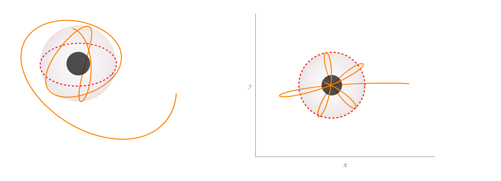
The analytical solutions with zero azimuthal angular momentum have additional simplifications for the homoclinic orbits. The roots of the angular potential in (57) reduce to

um+=1,um=ηma2(1γm2).u_{{m+}}=1\;,\quad u_{{m-}}=\frac{\eta_{m}}{a^{2}(1-\gamma^{2}_{m})}\,. (40)

The relevant root is um+=1u_{{m+}}=1 giving the two turning points at the north and south poles of a sphere, θm+=cos1(um+)=π\theta_{m+}=\cos^{-1}(-\sqrt{u_{m+}})={\pi} and θm=cos1(um+)=0\theta_{m-}=\cos^{-1}(\sqrt{u_{m+}})={0}, respectively [18]. Substitute (40) into the solution of θ(τm)\theta(\tau_{m}) in (60) and notice that um+/um1u_{m+}/u_{m-}\ll 1, since ηm\eta_{m} is relatively large value as seen in Fig.2, also aa and 1γm<11-\gamma_{m}<1. We can thus have the approximate solutions given by

θ(τm)\displaystyle\theta(\tau_{m}) =cos1(νθisn(ηm(τm+νθi𝒢θi)|um+um))\displaystyle=\cos^{-1}\left(-\nu_{\theta_{i}}{\rm sn}\left(\sqrt{\eta_{m}}\left(\tau_{m}+\nu_{\theta_{i}}{\mathcal{G}_{\theta_{i}}}\right)\left|\frac{u_{m+}}{u_{m-}}\right)\right.\right)
cos1(νθisin(ηm(τm+νθi𝒢θi))).\displaystyle\approx\cos^{-1}\left(-\nu_{\theta_{i}}{\rm sin}\left(\sqrt{\eta_{m}}\left(\tau_{m}+\nu_{\theta_{i}}{\mathcal{G}_{\theta_{i}}}\right)\right)\right)\;. (41)

By inspection, the angular velocity in Mino time of the evolution around the θ\theta can be read off as

ωθ=ηm.\omega_{\theta}=\sqrt{\eta_{m}}\;. (42)

In Fig. 5, we choose the initial conditions θi=π2\theta_{i}=\frac{\pi}{2} and νθi=1\nu_{\theta_{i}}=1, departing from the equator. Thus, with 𝒢θi=0{\mathcal{G}_{\theta_{i}}}=0 in (59), the solution just becomes θ(τm)=cos1(sin(ηmτm))\theta(\tau_{m})=\cos^{-1}\left(-{\rm sin}\left(\sqrt{\eta_{m}}\tau_{m}\right)\right). And, in Fig 6 the particle departs from the north pole with θi=0\theta_{i}=0 and νθi=1\nu_{\theta_{i}}=1, giving 𝒢θi=π2ηm{\mathcal{G}_{\theta_{i}}}=\frac{\pi}{2\sqrt{\eta_{m}}}. The evolution of coordinate θ\theta follows θ(τm)=cos1(cos(ηmτm))\theta(\tau_{m})=\cos^{-1}\left({\rm cos}\left(\sqrt{\eta_{m}}\tau_{m}\right)\right).

Refer to caption
Figure 6: Illustration of a zero azimuthal angular momentum homoclinic orbit with the parameters A in Fig. 2 and the initial conditions ri=rm4,θi=0r_{i}=r_{m4},\theta_{i}=0. The red dotted circle is on the equatorial plane.

As for the azimuthal motion, we notice that the equation of motion in (9) reduces to

dϕdτm=aγm[r2+a2Δ(r)1],\frac{d\phi}{d\tau_{m}}=a\gamma_{m}\left[\frac{r^{2}+a^{2}}{\Delta(r)}-1\right]\,, (43)

simply due to the frame dragging. In particular, the angular speed goes to a constant as rrmssr\rightarrow r_{\rm mss} when τm\tau_{m}\rightarrow\infty (tt\rightarrow\infty), given by

aγm[rmss2+a2Δ(rmss)1]ωϕ,ϕ(τm)=ωϕτm,a\gamma_{m}\left[\frac{r_{\rm mss}^{2}+a^{2}}{\Delta(r_{\rm mss})}-1\right]\equiv\omega_{\phi}\,,\quad\phi(\tau_{m})=\omega_{\phi}\tau_{m}\,, (44)

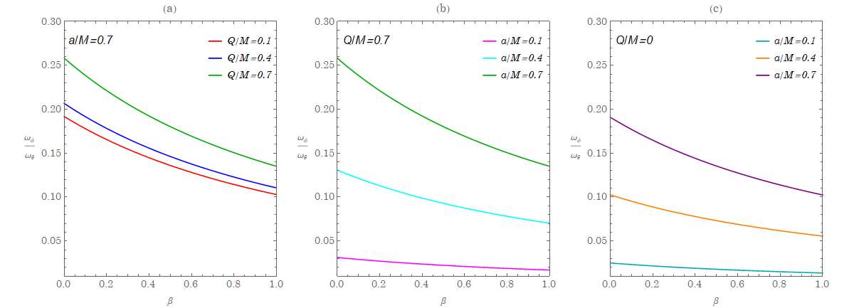
which can also be obtained directly from the analytical formulas (16) and (33) in the limits of λm=0\lambda_{m}=0 and τm\tau_{m}\rightarrow\infty (tt\rightarrow\infty). This allows one to plot the ratio of ωϕ\omega_{\phi} to ωθ\omega_{\theta} shown in Fig. 7. It is expected that the larger value of the black hole spin aa gives relatively large dragging effects and moreover, the charge QQ of the black hole gives the boost to it. This is consistent with the conclusion in the study of the particle boomerang in [18]. In there, we consider the spherical orbits of the particle with the radius of rmssr_{\rm mss} of the double root of the radial potential. For sufficiently large value of black hole spin aa there can be a particle boomerang that leaves the north polar axis (θ=0\theta=0) and travels along a constant-rr orbit to return to the north polar axis in precisely the opposite direction to that at which it leaves. The dragging of inertial frames rotates the particle propagation direction by an angle Δϕ=π\Delta\phi=\pi during one orbit that returns to the same location on the north polar axis. However, in the presence of the charge of the black hole in the Kerr-Newman black holes, the finite charge effect will enhance the frame dragging so as to reduce the needed value of the spin a to sustain Δϕ=π\Delta\phi=\pi.

Refer to caption
Figure 7: The ratio of ωϕ\omega_{\phi} to ωθ\omega_{\theta} given in (42) and (44) respectively as a function of β=rriscoribcorisco\beta=\frac{r-r_{\rm isco}}{r_{\rm ibco}-r_{\rm isco}} for Kerr-Newman black holes as well as Kerr black holes.

IV phase difference between nonequatorial Homoclinic orbits and spherical motion

According to [19], when the homoclinic orbits on the equatorial plane in Kerr black holes are considered, it is found a nontrivial fact that although as rr approaches to the unstable orbit, the accumulated phase ϕ\phi and time spent go to infinity. Nevertheless, the phase difference between the homoclinic orbits and the circular motion of the unstable orbits with the same radius of the double root turns out to be finite at time tt\rightarrow\infty, when both start at the same initial time. This will be also true for the homoclinic solution in the nonequatorial plane in the Kerr-Newman black holes where the circular motion is replaced by the spherical motion. As τm\tau_{m}\rightarrow\infty, giving tt\rightarrow\infty and rrmassr\rightarrow r_{\rm mass}, the radius of the unstable orbit, with the associated values of λmass,ηmass\lambda_{\rm mass},\eta_{\rm mass} obtained from (21) and (22), the phase difference becomes

Δϕτmdiff=ϕspheϕm\displaystyle\Delta\phi_{\tau_{m}}^{\rm diff}=\phi^{\rm sphe}-\phi_{m}
={a[(2MrmssQ2)aλm]Δ(rmss)τmIϕ(τm)}|τm\displaystyle=\left\{\frac{a\left[\left(2Mr_{\rm mss}-Q^{2}\right)-a\lambda_{m}\right]}{\Delta(r_{\rm mss})}\tau_{m}-I_{\phi}(\tau_{m})\right\}\Bigg{|}_{\tau_{m}\rightarrow\infty}
=2r+r(2Maγmrλm)r+Q2(aγmλm)(rmssr+)(1γm2)(r+rm1)(rm4r+)tanh1(r+rm1)(rm4rmss)(rm4r+)(rmssrm1)\displaystyle=\frac{2}{r_{+}-r_{-}}\frac{\left(2Ma\gamma_{m}-r_{-}\lambda_{m}\right)r_{+}-Q^{2}\left(a\gamma_{m}-\lambda_{m}\right)}{\left(r_{{\rm mss}}-r_{+}\right)\sqrt{\left(1-\gamma_{m}^{2}\right)\left(r_{+}-r_{m1}\right)\left(r_{m4}-r_{+}\right)}}\tanh^{-1}\sqrt{\frac{\left(r_{+}-r_{m1}\right)\left(r_{m4}-r_{\rm mss}\right)}{\left(r_{m4}-r_{+}\right)\left(r_{\rm mss}-r_{m1}\right)}}
2r+r(2Maγmr+λm)rQ2(aγmλm)(rmssr)(1γm2)(rrm1)(rm4r)tanh1(rrm1)(rm4rmss)(rm4r)(rmssrm1).\displaystyle-\frac{2}{r_{+}-r_{-}}\frac{\left(2Ma\gamma_{m}-r_{+}\lambda_{m}\right)r_{-}-Q^{2}\left(a\gamma_{m}-\lambda_{m}\right)}{\left(r_{{\rm mss}}-r_{-}\right)\sqrt{\left(1-\gamma_{m}^{2}\right)\left(r_{-}-r_{m1}\right)\left(r_{m4}-r_{-}\right)}}\tanh^{-1}\sqrt{\frac{\left(r_{-}-r_{m1}\right)\left(r_{m4}-r_{\rm mss}\right)}{\left(r_{m4}-r_{-}\right)\left(r_{\rm mss}-r_{m1}\right)}}\,. (45)

The general solutions of the homoclinic orbits and the spherical orbit contain the radial rr and angular θ\theta dependence seen from Eqs.(16) and (19). The θ\theta dependence cancels in computing Δϕτmdiff\Delta\phi_{\tau_{m}}^{\rm diff} and the only contributions come from the radial rr dependence. To obtain (IV), we have used the rr dependent solution of ϕ\phi (33) to the homoclinic orbits. Also, the radius of the spherical orbit is set at r=rmassr=r_{\rm mass} with the rr dependent solution obtained from (9) in terms of the Mino time in (14). For rmssr_{\rm mss} lying between rissor_{\rm isso} and ribcor_{\rm ibco} determined by (24) and (25), the corresponding λisso,ηisso\lambda_{\rm isso},\eta_{\rm isso} and λibso,ηibso\lambda_{\rm ibso},\eta_{\rm ibso} are determined by (21) and (22).

Refer to caption
Figure 8: Phase difference Δϕτmdiff=ϕspheϕm\Delta\phi_{\tau_{m}}^{\rm diff}=\phi^{\rm sphe}-\phi_{m} as a function of βλmss=|λibso||λmss||λibso||λisso|\beta_{\lambda_{\rm mss}}=\frac{|\lambda_{\rm ibso}|-|\lambda_{\rm mss}|}{|\lambda_{\rm ibso}|-|\lambda_{\rm isso}|} in (IV) for nonequatorial solutions. The upper plots are for the direct motion and the lower plots are for the retrograde motion.

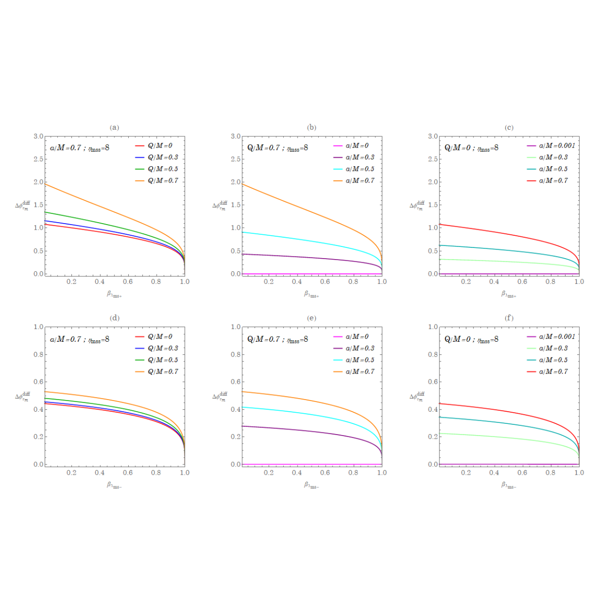
In Fig. 8, the phase difference is plotted as a function of βλmass\beta_{\lambda_{\rm mass}} defined by βλmass=|λmass||λisco||λibco||λisco|\beta_{\lambda_{\rm mass}}=\frac{{|\lambda_{\rm mass}}|-|\lambda_{\rm isco}|}{|\lambda_{\rm ibco}|-|\lambda_{\rm isco}|} for a fixed ηm\eta_{m}, which is the same value of ηm\eta_{m} at B in Fig. 2 allowing λm\lambda_{m} to vary. Since |λisco||λmass||λibco||\lambda_{\rm isco}|\leq|\lambda_{\rm mass}|\leq|\lambda_{\rm ibco}|, 0βλmass10\leq\beta_{\lambda_{\rm mass}}\leq 1. It is evident that the finite charge of the black hole will enhance the phase difference for both the direct motion (λmass>0\lambda_{\rm mass}>0) and retrograde motion (λmass<0\lambda_{\rm mass}<0). Also, for a fixed QQ, Δϕdiff\Delta\phi^{\rm diff} increases with the spin parameter aa of the black hole. This means that the homoclinic orbit moving toward the unstable orbit can synchronize with the circular motion in terms of the Mino time but in the end with a phase difference. This may provide useful information to construct the full spectrum of the gravitation waves in the case of EMRIs and is one of the interesting applications from the analytical solutions we obtain in this paper.

V equatorial homoclinic orbits

This section is devoted to the equatorial homoclinic solution, exemplified by the case C in Fig. 2 of the parameter space λm\lambda_{m} and ηm\eta_{m}. The main purpose here is to reduce our exact formulas for nonequatorial orbits to the expressions obtained in the context of the equatorial case. We will show some important steps to find their consistency. Since the results of [19] are written as a function rr, we begin with a useful relation between Mino time τm\tau_{m} and rr given by the inverse of (31),

τm(r)=2(1γm2)(rmssrm1)(rm4rmss)tanh1(xH(r)).\tau_{m}(r)=\frac{2}{\sqrt{(1-\gamma_{m}^{2})(r_{\rm mss}-r_{m1})(r_{m4}-r_{\rm mss})}}\tanh^{-1}\left({x^{H}(r)}\right)\,. (46)

For the proper time σm(r){\sigma_{m}(r)}, following (7) and (14) with Σ=r2\Sigma=r^{2} at the equatorial plane we then have

σm(r)σmi=rirr2±rRm(r)𝑑r=11γm2I2H(τm(r)).\sigma_{m}\left(r\right)-\sigma_{mi}=\int_{r_{i}}^{r}\frac{r^{2}}{\pm_{r}\sqrt{R_{m}(r)}}dr=\frac{1}{\sqrt{1-\gamma_{m}^{2}}}I_{2}^{H}\left(\tau_{m}\left(r\right)\right)\,. (47)

The term of I2HI^{H}_{2} given in (II.3) can be expressed by rr using (46). Rearranging them leads to

σm(r)\displaystyle\sigma_{m}\left(r\right) σmi=(rrmss)2(rm4r)(1γm2)(rrm1)+(rmssrm1)(rm4rmss)1γm2xH(r)\displaystyle-\sigma_{mi}=\sqrt{\frac{(r-r_{\rm mss})^{2}(r_{m4}-r)}{(1-\gamma_{m}^{2})(r-r_{m1})}}+\sqrt{\frac{(r_{\rm mss}-r_{m1})(r_{m4}-r_{\rm mss})}{1-\gamma_{m}^{2}}}x^{H}(r)
+(rm4rm1)(rm1+2rmss+rm4)(1γm2)(rmssrm1)(rm4rmss)hh1tanh1(hxH(r))\displaystyle+\frac{(r_{m4}-r_{m1})(r_{m1}+2r_{\rm mss}+r_{m4})}{\sqrt{(1-\gamma^{2}_{m})(r_{\rm mss}-r_{m1})(r_{m4}-r_{\rm mss})}}\frac{\sqrt{h}}{h-1}\tanh^{-1}\left(\sqrt{h}\;x^{H}(r)\right)
rmss(rm4rm1)rm1(rm4+rm1)+(rm4rm1)(rm1+2rmss+rm4)/(h1)1γm2(rmssrm1)(rm4rmss)tanh1(xH(r))\displaystyle-\frac{r_{\rm mss}(r_{m4}-r_{m1})-r_{m1}(r_{m4}+r_{m1})+(r_{m4}-r_{m1})(r_{m1}+2r_{\rm mss}+r_{m4})/(h-1)}{\sqrt{1-\gamma_{m}^{2}(r_{\rm mss}-r_{m1})(r_{m4}-r_{\rm mss})}}\tanh^{-1}\left(x^{H}(r)\right) (48)

Plugging in xH(r)x^{H}(r) and hh from (38) and (39), and doing a little algebra we arrive at

σm(r)σmi\displaystyle\sigma_{m}\left(r\right)-\sigma_{mi} =(rrm1)(rm4r)1γm2+2M(1γm2)3/2tan1rm4rrrm1\displaystyle=\sqrt{\frac{\left(r-r_{m1}\right)\left(r_{m4}-r\right)}{1-\gamma_{m}^{2}}}+\frac{2M}{\left(1-\gamma_{m}^{2}\right)^{3/2}}\tan^{-1}\sqrt{\frac{r_{m4}-r}{r-r_{m1}}}
+2(rmssrm1)(rmss+rm1)2(1γm2)(rm4rmss)tanh1(rmssrm1)(rm4r)(rm4rmss)(rrm1).\displaystyle+2\sqrt{\frac{\left(r_{\rm mss}-r_{m1}\right)\left(r_{\rm mss}+r_{m1}\right)^{2}}{\left(1-\gamma_{m}^{2}\right)\left(r_{m4}-r_{\rm mss}\right)}}\tanh^{-1}\sqrt{\frac{\left(r_{\rm mss}-r_{m1}\right)\left(r_{m4}-r\right)}{\left(r_{m4}-r_{\rm mss}\right)\left(r-r_{m1}\right)}}\,. (49)

This is the Kerr-Newman’s counterpart of equation (B66) in Ref. [19].

Taking the similar steps allows to obtain the equatorial homoclinic orbit in ϕ(r)\phi(r) coordinate. With the help of (9) evaluated at the equatorial plane and (14), we first rewrite

ϕ(r)ϕi=Iϕ(τm(r))+λmτm(r),{\phi}(r)-{\phi_{i}}={I_{\phi}}\left(\tau_{m}\left(r\right)\right)+\lambda_{m}\tau_{m}\left(r\right), (50)

where Iϕ{I_{\phi}} is given by (33) and τm\tau_{m} by (46). All the integrals for calculating ϕ(r){\phi}(r) are available from (II.3). The result can be written as follows

ϕm(r)ϕmi=2r+r𝒜tanh1(xH(r))++tanh1(h+xH(r))+tanh1(hrH(r))(1γm2)(rmscrm1)(rm4rmsc),\displaystyle\phi_{m}(r)-\phi_{mi}=\frac{2}{r_{+}-r_{-}}\frac{{\mathcal{A}\tanh^{-1}\left(x^{H}(r)\right)+\mathcal{B_{+}}\tanh^{-1}\left(\sqrt{h_{+}}x^{H}(r)\right)+\mathcal{B_{-}}\tanh^{-1}\left(\sqrt{h_{-}}r^{H}(r)\right)}}{\sqrt{(1-\gamma^{2}_{m})(r_{{\rm msc}}-r_{m1})(r_{m4}-r_{{\rm msc}})}}\,, (51)

where the coefficients 𝒜\mathcal{A} and ±\mathcal{B_{\pm}} are rr independent quantities involving the black hole parameters and the constants of motion of the particle, reading as

Refer to caption
Figure 9: Illustration of the equatorial homoclinic orbit of case C in Fig. 2. The red dotted circle is on the equatorial plane.
𝒜\displaystyle\mathcal{A} =λm(r+r)+2Maγmr+a2λmaγmQ2rm1r+[1rm1rm4(rm4r+)(h+1)]\displaystyle=\lambda_{m}\left(r_{+}-r_{-}\right)+\frac{2Ma\gamma_{m}r_{+}-a^{2}\lambda_{m}-a\gamma_{m}Q^{2}}{r_{m1}-r_{+}}\left[1-\frac{r_{m1}-r_{m4}}{(r_{m4}-r_{+})(h_{+}-1)}\right]
2Maγmra2λmaγmQ2rm1r[1rm1rm4(rm4r)(h1)],\displaystyle\quad\quad-\frac{2Ma\gamma_{m}r_{-}-a^{2}\lambda_{m}-a\gamma_{m}Q^{2}}{r_{m1}-r_{-}}\left[1-\frac{r_{m1}-r_{m4}}{(r_{m4}-r_{-})(h_{-}-1)}\right]\;, (52)

and

±=±(2Maγmr±a2λmaγmQ2)(rm1rm4)(rm1r±)(rm4r±)h±h±1.\displaystyle\mathcal{B_{\pm}}=\pm\frac{(2{M}a\gamma_{m}r_{\pm}-a^{2}{\lambda_{m}}-a{\gamma_{m}}Q^{2})(r_{m1}-r_{m4})}{(r_{m1}-r_{\pm})(r_{m4}-r_{\pm})}\frac{\sqrt{h_{\pm}}}{h_{\pm}-1}\;. (53)

Replacing xHx^{H} and h±h_{\pm} gives

ϕm(r)ϕmi=\displaystyle\;\;\phi_{m}\left(r\right)-\phi_{mi}=
2(rmscrm1)3(1γm2)(rm4rmsc)rmsc2λm+(2MrmscQ2)(aγmλm)(rmscr+)(rmscr)(rmscrm1)2tanh1(rmscrm1)(rm4r)(rm4rmsc)(rrm1)\displaystyle 2\sqrt{\frac{\left(r_{{\rm msc}}-r_{m1}\right)^{3}}{\left(1-\gamma_{m}^{2}\right)\left(r_{m4}-r_{{\rm msc}}\right)}}\frac{r_{{\rm msc}}^{2}\lambda_{m}+\left(2Mr_{{\rm msc}}-Q^{2}\right)\left(a\gamma_{m}-\lambda_{m}\right)}{\left(r_{{\rm msc}}-r_{+}\right)\left(r_{{\rm msc}}-r_{-}\right)\left(r_{{\rm msc}}-r_{m1}\right)^{2}}\tanh^{-1}\sqrt{\frac{\left(r_{{\rm msc}}-r_{m1}\right)\left(r_{m4}-r\right)}{\left(r_{m4}-r_{{\rm msc}}\right)\left(r-r_{m1}\right)}}
2r+r(2Maγmrλm)r+Q2(aγmλm)(rmscr+)(1γm2)(r+rm1)(rm4r+)tanh1(r+rm1)(rm4r)(rm4r+)(rrm1)\displaystyle-\frac{2}{r_{+}-r_{-}}\frac{\left(2Ma\gamma_{m}-r_{-}\lambda_{m}\right)r_{+}-Q^{2}\left(a\gamma_{m}-\lambda_{m}\right)}{\left(r_{{\rm msc}}-r_{+}\right)\sqrt{\left(1-\gamma_{m}^{2}\right)\left(r_{+}-r_{m1}\right)\left(r_{m4}-r_{+}\right)}}\tanh^{-1}\sqrt{\frac{\left(r_{+}-r_{m1}\right)\left(r_{m4}-r\right)}{\left(r_{m4}-r_{+}\right)\left(r-r_{m1}\right)}}
+2r+r(2Maγmr+λm)rQ2(aγmλm)(rmscr)(1γm2)(rrm1)(rm4r)tanh1(rrm1)(rm4r)(rm4r)(rrm1).\displaystyle+\frac{2}{r_{+}-r_{-}}\frac{\left(2Ma\gamma_{m}-r_{+}\lambda_{m}\right)r_{-}-Q^{2}\left(a\gamma_{m}-\lambda_{m}\right)}{\left(r_{{\rm msc}}-r_{-}\right)\sqrt{\left(1-\gamma_{m}^{2}\right)\left(r_{-}-r_{m1}\right)\left(r_{m4}-r_{-}\right)}}\tanh^{-1}\sqrt{\frac{\left(r_{-}-r_{m1}\right)\left(r_{m4}-r\right)}{\left(r_{m4}-r_{-}\right)\left(r-r_{m1}\right)}}\,. (54)

The derivation of t(r)t(r) is straightforward. From Eq. (10) at the equatorial plane and (14) we have found

tm(r)tmi=Imt(τm(r))\displaystyle t_{m}\left(r\right)-t_{mi}=I_{mt}\left(\tau_{m}\left(r\right)\right)
=γm(rrm1)(rm4r)1γm2+γmrm1+rm4+2(rmsc+2M)1γm2tan1rm4rrrm1\displaystyle=\gamma_{m}\sqrt{\frac{\left(r-r_{m1}\right)\left(r_{m4}-r\right)}{1-\gamma_{m}^{2}}}+\gamma_{m}\frac{r_{m1}+r_{m4}+2\left(r_{{\rm msc}}+2M\right)}{\sqrt{1-\gamma_{m}^{2}}}\tan^{-1}\sqrt{\frac{r_{m4}-r}{r-r_{m1}}}
+4(rmscrm1)3(1γm2)(rm4rmsc)rmsc2(rmsc2+a2)γm+(2MrmscQ2)(a2γmaλm)(rmscr+)(rmscr)(rmscrm1)2\displaystyle+\sqrt{\frac{4\left(r_{{\rm msc}}-r_{m1}\right)^{3}}{\left(1-\gamma_{m}^{2}\right)\left(r_{m4}-r_{{\rm msc}}\right)}}\frac{r_{{\rm msc}}^{2}\left(r_{{\rm msc}}^{2}+a^{2}\right)\gamma_{m}+\left(2Mr_{{\rm msc}}-Q^{2}\right)\left(a^{2}\gamma_{m}-a\lambda_{m}\right)}{\left(r_{{\rm msc}}-r_{+}\right)\left(r_{{\rm msc}}-r_{-}\right)\left(r_{{\rm msc}}-r_{m1}\right)^{2}}
×tanh1(rmscrm1)(rm4r)(rm4rmsc)(rrm1)\displaystyle\quad\quad\quad\quad\times\tanh^{-1}\sqrt{\frac{(r_{{\rm msc}}-r_{m1})\left(r_{m4}-r\right)}{\left(r_{m4}-r_{{\rm msc}}\right)\left(r-r_{m1}\right)}}
2(2Mr+Q2)r+r2Mγmr+(aλm+Q2γm)(rmscr+)(1γm2)(r+rm1)(rm4r+)tanh1(r+rm1)(rm4r)(rm4r+)(rrm1)\displaystyle-\frac{2\left(2Mr_{+}-Q^{2}\right)}{r_{+}-r_{-}}\frac{2M\gamma_{m}r_{+}-\left(a\lambda_{m}+Q^{2}\gamma_{m}\right)}{\left(r_{{\rm msc}}-r_{+}\right)\sqrt{\left(1-\gamma_{m}^{2}\right)\left(r_{+}-r_{m1}\right)\left(r_{m4}-r_{+}\right)}}\tanh^{-1}\sqrt{\frac{\left(r_{+}-r_{m1}\right)\left(r_{m4}-r\right)}{\left(r_{m4}-r_{+}\right)\left(r-r_{m1}\right)}}
+2(2MrQ2)r+r2Mγmr(aλm+Q2γm)(rmscr)(1γm2)(rrm1)(rm4r)tanh1(rrm1)(rm4r)(rm4r)(rrm1).\displaystyle+\frac{2\left(2Mr_{-}-Q^{2}\right)}{r_{+}-r_{-}}\frac{2M\gamma_{m}r_{-}-\left(a\lambda_{m}+Q^{2}\gamma_{m}\right)}{\left(r_{{\rm msc}}-r_{-}\right)\sqrt{\left(1-\gamma_{m}^{2}\right)\left(r_{-}-r_{m1}\right)\left(r_{m4}-r_{-}\right)}}\tanh^{-1}\sqrt{\frac{\left(r_{-}-r_{m1}\right)\left(r_{m4}-r\right)}{\left(r_{m4}-r_{-}\right)\left(r-r_{m1}\right)}}\,. (55)

In summary, the obtained formulas (V), (54), and (55) describe the equatorial homoclinic motion when the parameters and initial conditions are given. They are consistent with the results given in Appendix B of Ref. [19], as Q0Q\rightarrow 0 that results in rm1=0r_{m1}=0. Figure 9 shows an example of such an orbit for the solution given above. The parameters of the plot correspond to case C in Fig. 2.

Refer to caption
Figure 10: Phase difference Δϕτmdiff=ϕcircϕm\Delta\phi_{\tau_{m}}^{\rm diff}=\phi^{\rm circ}-\phi_{m} as a function of βλmsc=|λibco||λmsc||λibco||λisco|\beta_{\lambda_{\rm msc}}=\frac{|\lambda_{\rm ibco}|-|\lambda_{\rm msc}|}{|\lambda_{\rm ibco}|-|\lambda_{\rm isco}|} in (IV) for the case of equatorial solutions. The upper plots are for the direct motion and the lower plots are for the retrograde motion.

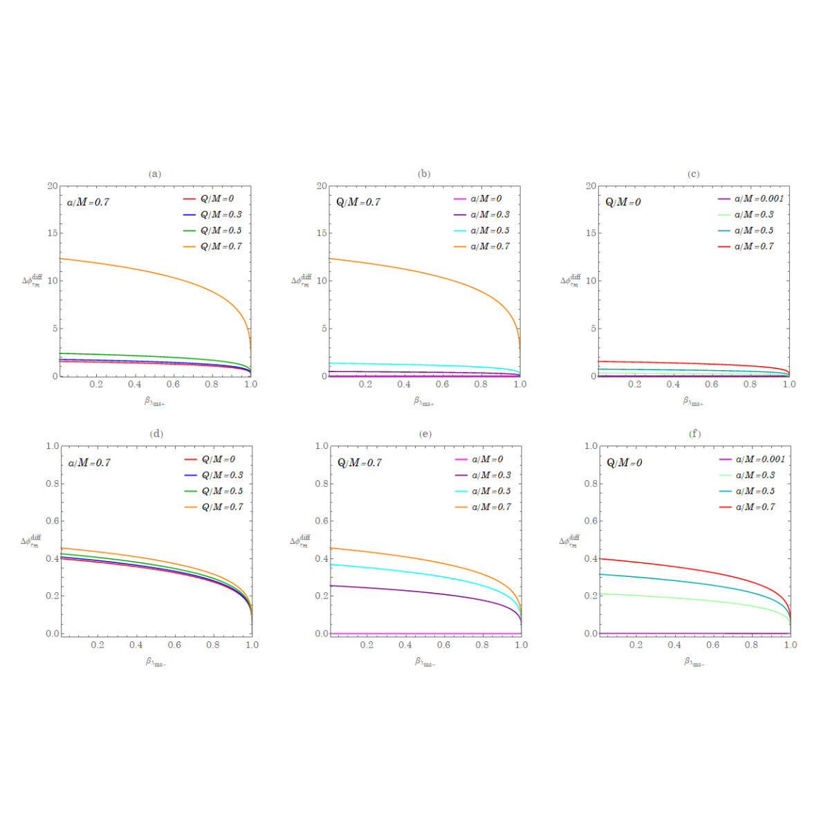
Figure 10 considers the phase difference between the homoclinic orbit and the circular motion on the equatorial plane in terms of the Mino time by taking ηmass0\eta_{\rm mass}\rightarrow 0 limit in Eq.(IV). The results of the Kerr cases are consistent with those in [19]. In addition, the study is extended to the black holes with finite charge to see the enhancement to the phase difference.

VI Summary and outlook

In this paper, we analytically derive the homoclinic solutions for the general nonequatorial orbits in the Kerr-Newman black holes. In the limits of Q0Q\rightarrow 0 and restricting on the equatorial plane, the obtained solution reduces to the one obtained in [19]. We then consider the homoclinic orbits with zero azimuthal angular momentum. The evolution of the ϕ\phi angle is solely due to the frame dragging effects. The larger value of the black hole spin aa gives relatively large dragging effects and moreover, the charge Q of the black hole gives the boost to it. Also, we compute the phase difference between the nonequatorial homoclinic solutions and the unstable spherical motion, giving the finite phase difference in terms of the Mino time as τm\tau_{m}\rightarrow\infty ( tt\rightarrow\infty), which might provide an interesting information to construct the full spectrum of the gravitational waves emitted by the EMRIs.

The existence of the homoclinic solutions which is separatrix between the motions of the inspiral types and plunging into the black holes gives the system to become chaotic when a random kick is acted on the particle [37]. The Lyapunov exponent for the chaotic system has been extensively investigated from the viewpoint of black hole systems with a probe particle based upon the AdS/CFT correspondence. According to the AdS/CFT duality in the case of the Schwarzschild black hole, it is claimed that there exists the bound on the Lyapunov exponent of such a probe particle [33]. Explicit calculations of the Lyapunov exponent will give insight on whether this conjecture of the bound on the Lyapunov exponent can be applied to the Kerr-Newman black holes. As long as any one of the evaluating Lyapunov exponents is a nonzero positive value at large time, we could probably see it as chaotic dynamics since the initial infinitesimal difference experiences exponential divergence eventually. Lastly, we can consider the system to experience an external time-dependent random noise from the random kicks, and are able to construct a Melnikov function. By taking advantage of the analytical expression of the homoclinic solution, the Melnikov function could be analytically solved. The simple zeros of the Melnikov function imply the occurrence of chaotic dynamics [22, 38].

Appendix A Angular potential Θ(θ)\Theta(\theta) and the integrals Gθ{G_{\theta}}, Gϕ{G_{\phi}}, and Gt{G_{t}}

For the sake of completeness, we summarize the relevant results related to the Θm\Theta_{m} potential in the θ\theta direction [35, 18]. The angular potential (13) for the particle can be rewritten in terms of u=cos2θu=\cos^{2}\theta as

(1u)Θm(u)=a2(γm21)u2+[a2(γm21)(ηm+λm2)]u+ηm.\displaystyle(1-u)\Theta_{m}(u)=-{a}^{2}\left(\gamma_{m}^{2}-1\right)u^{2}+\left[{a}^{2}\left(\gamma_{m}^{2}-1\right)-\left(\eta_{m}+\lambda_{m}^{2}\right)\right]u+\eta_{m}\,. (56)

The positivity of the Θm\Theta_{m} potential required λm\lambda_{m} and ηM\eta_{M} restricted in some parameter space (see Fig. 9 in [18]). The boundaries are determined from the roots of Θm(θ)=0\Theta_{m}(\theta)=0,

um±=Δmθ±Δmθ2+4a2ηm2a2,Δmθ=a2ηm+λm2γm21.\displaystyle u_{{m\pm}}=\frac{\Delta_{{m\theta}}\pm\sqrt{\Delta_{{m\theta}}^{2}+4\,{a}^{2}\,\eta_{m}}}{2{a}^{2}}\,,\quad\Delta_{m\theta}={a}^{2}-\frac{\eta_{m}+\lambda_{m}^{2}}{\gamma_{m}^{2}-1}\,. (57)

We consider the non-negative ηm0\eta_{m}\geq 0 for the orbits of the black hole exteriors and that requires the full trajectories lying in the Kerr-Newman black hole exterior [18]. For ηm>0\eta_{m}>0 and nonzero λm\lambda_{m} of the bound motion of the homoclinic orbits, 1>um+>01>u_{{m+}}>0 is the only positive root that in turn gives two roots at θm+=cos1(um+),θm=cos1(um+)\theta_{m+}=\cos^{-1}\left(-\sqrt{u_{{m+}}}\right),\theta_{m-}=\cos^{-1}\left(\sqrt{u_{{m+}}}\right). The particle travels between the southern and northern hemispheres crossing the equator. The corresponding solutions are expressed here as

τm=Gθ=p(𝒢θm+𝒢θm)+νθi[(1)p𝒢θ𝒢θi],\displaystyle\tau_{m}={G_{\theta}}=p({\mathcal{G}_{\theta_{m+}}}-{\mathcal{G}_{\theta_{m-}}})+\nu_{\theta_{i}}\left[(-1)^{p}{\mathcal{G}_{\theta}}-{\mathcal{G}_{\theta_{i}}}\right], (58)

where the trajectory passes through the turning point pp times and νθi=sign(dθidτm)\nu_{\theta_{i}}={\rm sign}\left(\frac{d\theta_{i}}{d{\tau_{m}}}\right). The function 𝒢θ{\mathcal{G}_{\theta}} is

𝒢θ=1uma2(γm21)F(sin1(cosθum+)|um+um).{\mathcal{G}_{\theta}}=-\frac{1}{\sqrt{-u_{m-}{a}^{2}\left(\gamma_{m}^{2}-1\right)}}F\left(\sin^{-1}\left(\frac{\cos\theta}{\sqrt{u_{m+}}}\right)\left|\frac{u_{m+}}{u_{m-}}\right)\right.\,. (59)

Inversion of (15) gives θ(τm)\theta(\tau_{m}) as [35, 18]

θ(τm)=cos1(νθium+sn(uma2(γm21)(τm+νθi𝒢θi)|um+um))\theta(\tau_{m})=\cos^{-1}\left(-\nu_{\theta_{i}}\sqrt{u_{m+}}{\rm sn}\left(\sqrt{-u_{m-}{a}^{2}\left(\gamma_{m}^{2}-1\right)}\left(\tau_{m}+\nu_{\theta_{i}}{\mathcal{G}_{\theta_{i}}}\right)\left|\frac{u_{m+}}{u_{m-}}\right)\right.\right) (60)

involving the Jacobi elliptic sine function [36].

The other two integrals related to G(θ)G(\theta) that contribute to the solutions of ϕ\phi and tt in (16) and (17) are

Gϕ(τm)\displaystyle{G_{\phi}}(\tau_{m}) =1uma2(γm21)Π(um+;am(uma2(γm21)(τm+νθi𝒢θi)|um+um)|um+um)\displaystyle=\frac{1}{\sqrt{-u_{m-}{a}^{2}\left(\gamma_{m}^{2}-1\right)}}\Pi\left(u_{m+};{\rm am}\left(\sqrt{-u_{m-}{a}^{2}\left(\gamma_{m}^{2}-1\right)}\left(\tau_{m}+\nu_{\theta_{i}}\mathcal{G}_{\theta_{i}}\right)\left|\frac{u_{m+}}{u_{m-}}\right)\right.\left|\frac{u_{m+}}{u_{m-}}\right)\right.
νθi𝒢ϕi,\displaystyle\quad-\nu_{\theta_{i}}{\mathcal{G}_{\phi_{i}}}\,, (61)

where

𝒢ϕi=1uma2(γm21)Π(um+;sin1(cosθium+)|um+um)\mathcal{G}_{\phi_{i}}=-\frac{1}{\sqrt{-u_{m-}{a}^{2}\left(\gamma_{m}^{2}-1\right)}}\Pi\left(u_{m+};\sin^{-1}\left(\frac{\cos\theta_{i}}{\sqrt{u_{m+}}}\right)\left|\frac{u_{m+}}{u_{m-}}\right)\right. (62)

and

Gt(τm)\displaystyle{G_{t}}(\tau_{m}) =2um+uma2(γm21)E(am(uma2(γm21)(τm+νθi𝒢θi)|um+um)|um+um)\displaystyle=-\frac{2u_{m+}}{\sqrt{-u_{m-}{a}^{2}\left(\gamma_{m}^{2}-1\right)}}E^{\prime}\left({\rm am}\left(\sqrt{-u_{m-}{a}^{2}\left(\gamma_{m}^{2}-1\right)}\left(\tau_{m}+\nu_{\theta_{i}}{\mathcal{G}_{\theta_{i}}}\right)\left|\frac{u_{m+}}{u_{m-}}\right)\right.\left|\frac{u_{m+}}{u_{m-}}\right)\right.
νθi𝒢ti,\displaystyle\quad-\nu_{\theta_{i}}\mathcal{G}_{t_{i}}\,, (63)

where

𝒢ti=2um+uma2(γm21)E(sin1(cosθiu+)|um+um).\mathcal{G}_{t_{i}}=\frac{2u_{m+}}{\sqrt{-u_{m-}{a}^{2}\left(\gamma_{m}^{2}-1\right)}}E^{\prime}\left(\sin^{-1}\left(\frac{\cos\theta_{i}}{\sqrt{u_{+}}}\right)\left|{\frac{u_{m+}}{u_{m-}}}\right)\right.\,. (64)

The results above also involve incomplete elliptic integrals of the second and third kinds. The derivative of E(φk)E(\varphi\mid k) can be calculated through

E(φ|k)=kE(φ|k)=E(φ|k)F(φ|k)2k.\displaystyle E^{\prime}\left(\varphi\left|k\right)\right.=\partial_{k}E\left(\varphi\left|k\right)\right.=\frac{E\left(\varphi\left|k\right)\right.-F\left(\varphi\left|k\right)\right.}{2k}\,. (65)

Notice that since 0<um+um<10<\frac{u_{m+}}{u_{m-}}<1 for the bound motion, the involved elliptic functions are all real valued and finite. In particular, for ηm=0\eta_{m}=0, the orbits are on the equatorial plane at θ=π2\theta=\frac{\pi}{2}.

Appendix B Radial potential Rm(r)R_{m}(r) and the integrals Iθ{I_{\theta}}, Iϕ{I_{\phi}}, and It{I_{t}}

As for the radial potential, we examine the parameter space to have positive Rm(r)R_{m}({r}). It is a quartic function of the form [18]

Rm(r)=Smr4+Tmr3+Umr2+Vmr+Wm,\displaystyle R_{m}({r})=S_{m}{r}^{4}+T_{m}{r}^{3}+U_{m}{r}^{2}+V_{m}{r}+W_{m}\,, (66)

where the coefficients are written in terms of the black hole parameters and the constants of motion,

Sm=γm21,\displaystyle S_{m}=\gamma_{m}^{2}-1, (67)
Tm=2M,\displaystyle T_{m}=2M, (68)
Um=a2(γm21)Q2ηmλm2,\displaystyle U_{m}={a}^{2}\left(\gamma_{m}^{2}-1\right)-{Q}^{2}-\eta_{m}-\lambda_{m}^{2}, (69)
Vm=2M[(aγmλm)2+ηm],\displaystyle V_{m}=2M\Bigl{[}\left({a}\gamma_{m}-\lambda_{m}\right)^{2}+\eta_{m}\Bigr{]}, (70)
Wm=a2ηmQ2[(aγmλm)2+ηm].\displaystyle W_{m}=-{a}^{2}\eta_{m}-{Q}^{2}\Bigl{[}\left({a}\gamma_{m}-\lambda_{m}\right)^{2}+\eta_{m}\Bigr{]}\,. (71)

We name the roots as Rm(r)=(γm21)(rrm1)(rrm2)(rrm3)(rrm4)R_{m}({r})=\left(\gamma_{m}^{2}-1\right)({r}-r_{m1})({r}-r_{m2})({r}-r_{m3})({r}-r_{m4}), being (rm4>rm3>rm2>rm1)\left(r_{m4}>r_{m3}>r_{m2}>r_{m1}\right). The explicit formulas of the roots are cumbersome, we summarize them below:

rm1=M2(γm21)zmXm2zm2+Ym4zm,r_{m1}=-\frac{M}{2\left(\gamma_{m}^{2}-1\right)}-z_{m}-\sqrt{-\hskip 2.84526pt\frac{{X}_{m}}{2}-z_{m}^{2}+\frac{{Y}_{m}}{4z_{m}}}\,, (72)
rm2=M2(γm21)zm+Xm2zm2+Ym4zm,r_{m2}=-\frac{M}{2\left(\gamma_{m}^{2}-1\right)}-z_{m}+\sqrt{-\hskip 2.84526pt\frac{{X}_{m}}{2}-z_{m}^{2}+\frac{{Y}_{m}}{4z_{m}}}\,, (73)
rm3=M2(γm21)+zmXm2zm2Ym4zm,r_{m3}=-\frac{M}{2\left(\gamma_{m}^{2}-1\right)}+z_{m}-\sqrt{-\hskip 2.84526pt\frac{{X}_{m}}{2}-z_{m}^{2}-\frac{{Y}_{m}}{4z_{m}}}\,, (74)
rm4=M2(γm21)+zm+Xm2zm2Ym4zm,r_{m4}=-\frac{M}{2\left(\gamma_{m}^{2}-1\right)}+z_{m}+\sqrt{-\hskip 2.84526pt\frac{{X}_{m}}{2}-z_{m}^{2}-\frac{{Y}_{m}}{4z_{m}}}\,, (75)

where

zm=Ωm++ΩmXm32,Ωm±=ϰm2±(ϖm3)3+(ϰm2)23z_{m}=\sqrt{\frac{\Omega_{m+}+\Omega_{m-}-\frac{{X}_{m}}{3}}{2}}\;,\quad\Omega_{m\pm}=\sqrt[3]{-\hskip 2.84526pt\frac{{\varkappa}_{m}}{2}\pm\sqrt{\left(\frac{{\varpi}_{m}}{3}\right)^{3}+\left(\frac{{\varkappa}_{m}}{2}\right)^{2}}}\, (76)

with

ϖm=Xm212Zm,ϰm=Xm3[(Xm6)2Zm]Ym28.{\varpi}_{m}=-\hskip 2.84526pt\frac{{X}_{m}^{2}}{12}-{Z}_{m}\,,\quad\quad{\varkappa}_{m}=-\hskip 2.84526pt\frac{{X}_{m}}{3}\left[\left(\frac{{X}_{m}}{6}\right)^{2}-{Z}_{m}\right]-\hskip 2.84526pt\frac{{Y}_{m}^{2}}{8}\,. (77)

XmX_{m}, YmY_{m}, and ZmZ_{m} are the short notation for

Xm=8UmSm3Tm28Sm2,\displaystyle{X}_{m}=\frac{8U_{m}S_{m}-3T_{m}^{2}}{8S_{m}^{2}}\,, (78)
Ym=Tm34UmTmSm+8VmSm28Sm3,\displaystyle{Y}_{m}=\frac{T_{m}^{3}-4U_{m}T_{m}S_{m}+8V_{m}S_{m}^{2}}{8S_{m}^{3}}\,, (79)
Zm=3Tm4+256WmSm364VmTmSm2+16UmTm2Sm256Sm4.\displaystyle{Z}_{m}=\frac{-3T_{m}^{4}+256W_{m}S_{m}^{3}-64V_{m}T_{m}S_{m}^{2}+16U_{m}T_{m}^{2}S_{m}}{256S_{m}^{4}}\,. (80)

The sum of the roots satisfies the relation rm1+rm2+rm3+rm4=2γm21r_{m1}+r_{m2}+r_{m3}+r_{m4}=-\frac{2}{\gamma_{m}^{2}-1}\;. Some of the feature of RmR_{m} is illustrated in Fig. 1. See also Fig. 10 in [18].

We at this stage show an analytical solution of bound orbits, where rm3rirm4r_{m3}\leq r_{i}\leq r_{m4}, which is suited to constructing the homoclinic solution discussed in Sec. II.3. The bound solution of r(τm)r(\tau_{m}) is given by the inversion of (17),

r(τm)=rm4(rm1rm3)rm1(rm4rm3)sn2(XB(τm)|kB)(rm1rm3)(rm4rm3)sn2(XB(τm)|kB),r(\tau_{m})=\frac{r_{m4}(r_{m1}-r_{m3})-r_{m1}(r_{m4}-r_{m3}){\rm sn}^{2}\left(X^{B}(\tau_{m})\left|k^{B}\right)\right.}{(r_{m1}-r_{m3})-(r_{m4}-r_{m3}){\rm sn}^{2}\left(X^{B}(\tau_{m})\left|k^{B}\right)\right.}\,, (81)

where

XB(τm)=(1γm2)(rm3rm1)(rm4rm2)2τmνriF(sin1((rirm4)(rm1rm3)(rirm1)(rm4rm3))|kB)X^{B}(\tau_{m})=\frac{\sqrt{\left(1-\gamma_{m}^{2}\right)(r_{m3}-r_{m1})(r_{m4}-r_{m2})}}{2}\tau_{m}-\nu_{r_{i}}F\Bigg{(}\sin^{-1}\left(\sqrt{\frac{(r_{i}-r_{m4})(r_{m1}-r_{m3})}{(r_{i}-r_{m1})(r_{m4}-r_{m3})}}\right)\left|k^{B}\Bigg{)}\right.\,\\ (82)

and

kB=(rm4rm3)(rm2rm1)(rm4rm2)(rm3rm1).k^{B}=\frac{(r_{m4}-r_{m3})(r_{m2}-r_{m1})}{(r_{m4}-r_{m2})(r_{m3}-r_{m1})}\,. (83)

with νri=sign(dridτm)\nu_{r_{i}}={\rm sign}\left(\frac{dr_{i}}{d{\tau_{m}}}\right) and sn\rm sn denoting the Jacobi elliptic sine function.

The other integrals involving the radial potential Rm(r)R_{m}(r) are obtained as

IϕB(τm)=γm1γm22Mar+r[(r+a(λmγm)+Q22M)I+B(τm)(ra(λmγm)+Q22M)IB(τm)],I^{B}_{\phi}(\tau_{m})=\frac{\gamma_{m}}{\sqrt{1-\gamma_{m}^{2}}}\frac{2Ma}{r_{+}-r_{-}}\left[\left(r_{+}-\frac{a\left(\frac{\lambda_{m}}{\gamma_{m}}\right)+Q^{2}}{2M}\right)I_{+}^{B}(\tau_{m})-\left(r_{-}-\frac{a\left(\frac{\lambda_{m}}{\gamma_{m}}\right)+Q^{2}}{2M}\right)I_{-}^{B}(\tau_{m})\right]\,, (84)
ItB(τm)=γm1γm2{4M2r+r[(r+Q22M)(r+a(λmγm)+Q22M)I+B(τm)\displaystyle I^{B}_{t}(\tau_{m})=\frac{\gamma_{m}}{\sqrt{1-\gamma_{m}^{2}}}\left\{\frac{4M^{2}}{r_{+}-r_{-}}\left[\left(r_{+}-\frac{Q^{2}}{2M}\right)\left(r_{+}-\frac{a\left(\frac{\lambda_{m}}{\gamma_{m}}\right)+Q^{2}}{2M}\right)I_{+}^{B}(\tau_{m})\right.\right.
(rQ22M)(ra(λmγm)+Q22M)IB(τm)]+2MI1B(τm)+I2B(τm)}+(4M2Q2)γmτm,\displaystyle\quad\quad\left.\left.-\left(r_{-}-\frac{Q^{2}}{2M}\right)\left(r_{-}-\frac{a\left(\frac{\lambda_{m}}{\gamma_{m}}\right)+Q^{2}}{2M}\right)I_{-}^{B}(\tau_{m})\right]+2MI_{1}^{B}(\tau_{m})+I_{2}^{B}(\tau_{m})\right\}+\left(4{M^{2}}-Q^{2}\right)\gamma_{m}\tau_{m}\,, (85)

where

I±B(τm)=2(rm3rm1)(rm4rm2)[XB(τm)rm1r±+rm1rm4(rm1r±)(rm4r±)Π(β±;ΥτmB|kB)]+νri±iB\displaystyle I_{\pm}^{B}(\tau_{m})=\frac{2}{\sqrt{(r_{m3}-r_{m1})(r_{m4}-r_{m2})}}\left[\frac{X^{B}(\tau_{m})}{r_{m1}-r_{\pm}}+\frac{r_{m1}-r_{m4}}{(r_{m1}-r_{\pm})(r_{m4}-r_{\pm})}\Pi\left(\beta_{\pm};\Upsilon_{\tau_{m}}^{B}\left|k^{B}\right)\right.\right]+\nu_{r_{i}}\mathcal{I}_{\pm_{i}}^{B} (86)
±iB=2(rm3rm1)(rm4rm2)[F(ΥriBkB)rm1r±+rm1rm4(rm1r±)(rm4r±)Π(β±;ΥriB|kB)]\displaystyle\mathcal{I}_{\pm_{i}}^{B}=\frac{2}{\sqrt{(r_{m3}-r_{m1})(r_{m4}-r_{m2})}}\left[\frac{F\left(\Upsilon_{r_{i}}^{B}\mid k_{B}\right)}{r_{m1}-r_{\pm}}+\frac{r_{m1}-r_{m4}}{(r_{m1}-r_{\pm})(r_{m4}-r_{\pm})}\Pi\left(\beta_{\pm};\Upsilon_{r_{i}}^{B}\left|k_{B}\right)\right.\right] (87)
I1B(τm)=2(rm3rm1)(rm4rm2)[rm1XB(τm)+(rm4rm1)Π(β;ΥτmB|kB)]+νri1iB\displaystyle I_{1}^{B}(\tau_{m})=\frac{2}{\sqrt{(r_{m3}-r_{m1})(r_{m4}-r_{m2})}}\left[r_{m1}X^{B}(\tau_{m})+(r_{m4}-r_{m1})\Pi\left(\beta;\Upsilon_{\tau_{m}}^{B}\left|k^{B}\right)\right.\right]+\nu_{r_{i}}\mathcal{I}_{1_{i}}^{B} (88)
1iB=2(rm3rm1)(rm4rm2)[rm1F(ΥriB|kB)+(rm4rm1)Π(β;ΥriB|kB)]\displaystyle\mathcal{I}_{1_{i}}^{B}=\frac{2}{\sqrt{(r_{m3}-r_{m1})(r_{m4}-r_{m2})}}\left[r_{m1}F\left(\Upsilon_{r_{i}}^{B}\left|k_{B}\right)\right.+(r_{m4}-r_{m1})\Pi\left(\beta;\Upsilon_{r_{i}}^{B}\left|k_{B}\right)\right.\right] (89)
I2B(τm)=νr(r(τm)rm1)(r(τm)rm2)(r(τm)rm3)(rm4r(τm))r(τm)rm1\displaystyle I_{2}^{B}(\tau_{m})=-\nu_{r}\frac{\sqrt{\left(r(\tau_{m})-r_{m1}\right)\left(r(\tau_{m})-r_{m2}\right)\left(r(\tau_{m})-r_{m3}\right)\left(r_{m4}-r(\tau_{m})\right)}}{r(\tau_{m})-r_{m1}}
rm3(rm4rm1)rm1(rm4+rm1)(rm3rm1)(rm4rm2)XB(τm)+(rm3rm1)(rm4rm2)E(ΥτmB|kB)\displaystyle\quad\quad-\frac{r_{m3}\left(r_{m4}-r_{m1}\right)-r_{m1}\left(r_{m4}+r_{m1}\right)}{\sqrt{(r_{m3}-r_{m1})(r_{m4}-r_{m2})}}X^{B}(\tau_{m})+\sqrt{(r_{m3}-r_{m1})(r_{m4}-r_{m2})}E\left(\Upsilon_{\tau_{m}}^{B}\left|k^{B}\right)\right.
+(rm4rm1)(rm1+rm2+rm3+rm4)(rm3rm1)(rm4rm2)Π(β;ΥτmB|kB)+νri2iB\displaystyle\quad\quad+\frac{\left(r_{m4}-r_{m1}\right)\left(r_{m1}+r_{m2}+r_{m3}+r_{m4}\right)}{\sqrt{(r_{m3}-r_{m1})(r_{m4}-r_{m2})}}\Pi\left(\beta;\Upsilon_{\tau_{m}}^{B}\left|k^{B}\right)\right.+\nu_{r_{i}}\mathcal{I}_{2_{i}}^{B} (90)
2iB=(rirm1)(rirm2)(rirm3)(rm4ri)rirm1rm3(rm4rm1)rm1(rm4+rm1)(rm3rm1)(rm4rm2)F(ΥriB|kB)\displaystyle\mathcal{I}_{2_{i}}^{B}=\frac{\sqrt{\left(r_{i}-r_{m1}\right)\left(r_{i}-r_{m2}\right)\left(r_{i}-r_{m3}\right)\left(r_{m4}-r_{i}\right)}}{r_{i}-r_{m1}}-\frac{r_{m3}\left(r_{m4}-r_{m1}\right)-r_{m1}\left(r_{m4}+r_{m1}\right)}{\sqrt{(r_{m3}-r_{m1})(r_{m4}-r_{m2})}}F\left(\Upsilon_{r_{i}}^{B}\left|k^{B}\right)\right.
+(rm3rm1)(rm4rm2)E(ΥriB|kB)+(rm4rm1)(rm1+rm2+rm3+rm4)(rm3rm1)(rm4rm2)Π(β;ΥriB|kB)\displaystyle\quad\quad+\sqrt{(r_{m3}-r_{m1})(r_{m4}-r_{m2})}E\left(\Upsilon_{r_{i}}^{B}\left|k^{B}\right)\right.+\frac{\left(r_{m4}-r_{m1}\right)\left(r_{m1}+r_{m2}+r_{m3}+r_{m4}\right)}{\sqrt{(r_{m3}-r_{m1})(r_{m4}-r_{m2})}}\Pi\left(\beta;\Upsilon_{r_{i}}^{B}\left|k^{B}\right)\right. (91)

The parameters in the equations above are

ΥrB=sin1(rrm4)(rm1rm3)(rrm1)(rm4rm3),ΥτmB=am(XB(τm)|kB)\displaystyle\Upsilon_{r}^{B}=\sin^{-1}\sqrt{\frac{(r-r_{m4})(r_{m1}-r_{m3})}{(r-r_{m1})(r_{m4}-r_{m3})}},\hskip 11.38109pt\Upsilon_{\tau_{m}}^{B}={\rm am}\bigl{(}X^{B}(\tau_{m})\left|k_{B}\bigr{)}\right. (92)
νr=sign(dr(τm)dτm),β±B=(rm1r±)(rm4rm3)(rm4r±)(rm1rm3),βB=rm4rm3rm1rm3.\displaystyle\nu_{r}={\rm sign}\left(\frac{dr(\tau_{m})}{d\tau_{m}}\right),\hskip 11.38109pt\beta^{B}_{\pm}=\frac{(r_{m1}-r_{\pm})(r_{m4}-r_{m3})}{(r_{m4}-r_{\pm})(r_{m1}-r_{m3})},\hskip 11.38109pt\beta^{B}=\frac{r_{m4}-r_{m3}}{r_{m1}-r_{m3}}\,. (93)
Acknowledgements.
This work was supported in part by the National Science and Technology Council (NSTC) of Taiwan, Republic of China.

References

  • [1] B. P. Abbott et al. (LIGO Scientific and Virgo Collaborations), Observation of Gravitational Waves from a Binary Black Hole Merger, Phys. Rev. Lett. 116, 061102 (2016).
  • [2] B. P. Abbott et al. (LIGO Scientific and Virgo Collaborations), GWTC-1: A Gravitational-Wave Transient Catalog of Compact Binary Mergers Observed by LIGO and Virgo during the First and Second Observing Runs, Phys. Rev. X 9, 031040 (2019).
  • [3] R. Abbott et al. (LIGO Scientific and Virgo Collaborations), GWTC-2: Compact Binary Coalescences Observed by LIGO and Virgo during the First Half of the Third Observing Run, Phys. Rev. X 11, 021053 (2021).
  • [4] K. Akiyama et al. (Event Horizon Telescope), First M87 Event Horizon Telescope Results. I. The Shadow of the Supermassive Black Hole, Astrophys. J. 875, L1 (2019).
  • [5] K. Akiyama et al. (Event Horizon Telescope), First Sagittarius A* Event Horizon Telescope Results. I. The Shadow of the Supermassive Black Hole in the Center of the Milky Way, Astrophys. J. Lett. 930, L12 (2022).
  • [6] C. W. Misner, K. S. Thorne, and J. A. Wheeler, Gravitation (W. H. Freeman and Company, San Francisco, 1973).
  • [7] S. Chandrasekhar, The Mathematical Theory of Black Holes, International Series of Monographs on Physics (Clarendon Press/Oxford University Press, 1992).
  • [8] eLISA Consortium et al., The gravitational universe, arXiv:1305.5720.
  • [9] Enrico Barausse et al., Prospects for fundamental physics with LISA, Gen. Relativ. Gravit. 52, 81 (2020).
  • [10] Stanislav Babak et al., Science with the space-based interferometer LISA. V. Extreme mass-ratio inspirals, Phys.Rev.D 95, 103012 (2017).
  • [11] Bence Kocsis, Nicolas Yunes,and Abraham Loeb, Observable signatures of extreme mass-ratio in spiral black hole binaries embedded in thin accretion disks, Phys. Rev.D 84, 024032 (2011).
  • [12] B. Carter, Global structure of the Kerr family of gravitational fields, Phys. Rev. 174, 1559 (1968).
  • [13] Y. Mino, Perturbative approach to an orbital evolution around a supermassive black hole, Phys. Rev. D 67, 084027 (2003).
  • [14] T. Damour, R. Hanni, R. Ruffini, and J. Wilson, Regions of magnetic support of a plasma around a black hole, Phys. Rev. D 17, 1518 (1978).
  • [15] R. Abuter, et al. (GRAVITY Collaboration), Detection of orbital motions near the last stable circular orbit of the massive black hole SgrA* Astronom. Astrophys. 618, L10 (2018).
  • [16] M. Zajacek, A. Tursunov, A. Eckart, and S. Britzen, On the charge of the Galactic centre black hole, Mon. Not. R. Astron. Soc. 480, 4408 (2018).
  • [17] M. Zajacek, A. Tursunov, A. Eckart, S. Britzen, E. Hackmann, V. Karas, Z. Stuchlik, B. Czerny, J.A. Zensus, Constraining the charge of the Galactic Centre black hole, J. Phys. Conf. Ser. 1258, 012031 (2019).
  • [18] Chen-Yu Wang, Da-Shin Lee, and Chi-Yong Lin, Null and time-like geodesics in Kerr-Newman black hole exterior, Phys. Rev. D 106, 084048 (2022).
  • [19] Janna Levin, Gabe Perez-Giz, Homoclinic orbits around spinning black holes I: Exact solution for the Kerr separatrix, Phys. Rev. D 79, 124013 (2009).
  • [20] R. O’Shaughnessy, Transition from inspiral to plunge for eccentric equatorial Kerr orbits, Phys. Rev. 67, 044004, (2003).
  • [21] U. Sperhake, E. Berti, V. Cardoso, J. A. Gonzalez, B. Bruegmann, M. Ansorg, Eccentric binary black-hole mergers: The transition from inspiral to plunge in general relativity, Phys. Rev. D 78, 064069 (2008).
  • [22] L Bombelli and E Calzetta, Chaos around a black hole, Classical Quantum Gravity, 9, 2573 (1992).
  • [23] Kostas Glampedakis, Scott A. Hughes, and Daniel Kennefick, Approximating the inspiral of test bodies into Kerr black holes, Phys. Rev. D 66, 064055 (2002).
  • [24] Steve Drasco and Scott A. Hughes, Rotating black hole orbit functionals in the frequency domain, Phys. Rev. D 69, 044015 (2004).
  • [25] Steve Drasco, Éanna É Flanagan, and Scott A Hughes, Computing inspirals in Kerr in the adiabatic regime: I. The scalar case, Classical Quantum Gravity 22, S801 (2005).
  • [26] Steve Drasco, Scott A. Hughes, Gravitational wave snapshots of generic extreme mass ratio inspirals, Phys. Rev. D 73, 024027 (2006).
  • [27] Ryan N. Lang and Scott A. Hughes, Measuring coalescing massive binary black holes with gravitational waves: The impact of spin-induced precession, Phys. Rev. D 74, 122001 (2006).
  • [28] Nathan A. Collins, Scott A. Hughes, Towards a formalism for mapping the spacetimes of massive compact objects: Bumpy black holes and their orbits, Phys. Rev. D 69, 124022 (2004).
  • [29] Steve Drasco, Strategies for observing extreme mass ratio inspirals, Classical Quantum Gravity 23, S769 (2006).
  • [30] Janna Levin, Rachel O’Reilly, and E. J. Copeland, Gravity waves from homoclinic orbits of compact binaries, Phys. Rev. D 62, 024023 (2000).
  • [31] Janna Levin, Gravity Waves, Chaos, and Spinning Compact Binaries, Phys. Rev. Lett. 84, 3515 (2000).
  • [32] Janna Levin, Fate of chaotic binaries, Phys. Rev. D 67, 044013 (2003).
  • [33] J. Maldacena, S. H. Shenker, and D. Stanford, A bound on chaos, J. High Energy Phys. 08, 106 (2016).
  • [34] D. C. Wilkins, Bound geodesics in the Kerr metric, Phys. Rev. D 5, 814 (1972).
  • [35] S. E. Gralla and A. Lupsasca, Null geodesics of the Kerr exterior, Phys. Rev. D 101, 044032 (2020).
  • [36] M. Abramowitz and I. A. Stegun, Handbook of Mathematical Functions with Formulas, Graphs, and Mathematical Tables, 9th ed. (Dover, New York, 1964).
  • [37] Chen-Yu Liu, Da-Shin Lee and Chi-Yong Lin, Geodesic motion of neutral particles around a Kerr–Newman black hole, Classical Quantum Gravity 34, 235008 (2017).
  • [38] Wei-Can Syu, Da-Shin Lee, and Chi-Yong Lin, Regular and chaotic behavior of collective atomic motion in two-component Bose-Einstein condensates, Phys. Rev. A 101, 063622 (2020).