Homological stability for generalized Hurwitz spaces and Selmer groups in quadratic twist families over function fields
Abstract.
We prove a version of the Bhargava-Kane-Lenstra-Poonen-Rains heuristics for Selmer groups of quadratic twist families of abelian varieties over global function fields. As a consequence, we derive a result towards the “minimalist conjecture" on Selmer ranks of abelian varieties in such families. More precisely, we show that the probabilities predicted in these two conjectures are correct to within an error term in the size of the constant field, , which goes to as grows. Two key inputs are a new homological stability theorem for a generalized version of Hurwitz spaces parameterizing covers of punctured Riemann surfaces of arbitrary genus, and an expression of average sizes of Selmer groups in terms of the number of rational points on these Hurwitz spaces over finite fields.
Key words and phrases:
Bhargava-Kane-Lenstra-Poonen-Rains heuristics, the minimalist conjecture, quadratic twists, homological stability, big monodromy2020 Mathematics Subject Classification:
Primary 11G05; Secondary 11G10, 14G15, 55N991. Introduction
For a positive integer and an abelian variety over a global field , the Selmer group of , denoted , is a group which sits in an exact sequence between the mod Mordell-Weil group and the torsion in the Tate-Shafarevich group . These Selmer groups, unlike the other two terms in the exact sequence, are computationally approachable, and provide the most tractable means of obtaining information about the rank of and of .
The Selmer group of an abelian variety can be thought of as a higher analogue of the class group of a number field. The behavior of the class group of a number field chosen at random from a specified family is the subject of the Cohen-Lenstra conjecture and its many subsequent generalizations. In the same way, the question “what does the Selmer group of a random abelian variety look like?" is the subject of a suite of more recent conjectures. Conjectures predicting the distribution of Selmer groups were formulated in [PR12], when is prime, and generalized to the case of composite in [BKL+15, §5.7], see also [FLR23, §5.3.3]. We call these conjectures the “BKLPR heuristics.” Although the above papers state their conjectures in the context of the universal family parameterizing all elliptic curves, it is also natural to ask under what circumstances they apply to quadratic twist families ( [PR12, Remark 1.9].) Our main result is a proof of these conjectures over function fields of arbitrary genus, up to an error term in that approaches as grows, in the case where the family of abelian varieties is the family of quadratic twists of a fixed abelian variety.
For a suitably large prime, as an immediate consequence of our main result, we obtain a version of the minimalist conjecture for Selmer ranks, which predicts that quadratic twists of a fixed elliptic curve have Selmer rank half the time, Selmer rank half the time, and Selmer rank at least zero percent of the time.
The approach of this paper is similar to that of [EVW16], which verifies a version of the Cohen-Lenstra heuristics over genus function fields. As in [EVW16], one key input is a new homological stability theorem. This theorem, which is purely topological in nature, is used to bound the étale cohomology of relevant moduli spaces, whose points count elements of Selmer groups of quadratic twists of an abelian variety.
1.1. Main Results
To give an indication of the nature of the results we prove in this paper, we start with a very special case of Theorem 1.1.3 below, see 1.1.6. We now describe this special case informally. Let be a finite field of odd characteristic, be an abelian variety over the field with good reduction over , and an odd prime not dividing . For any squarefree polynomial of even degree ,111See 1.4.6 for a discussion on how to generalize this to the case that the degree, , is odd. we denote by the quadratic twist of by the quadratic character of associated to . Write for the average size of the Selmer group of as ranges over squarefree polynomials of degree which are coprime to the bad reduction locus of . Similarly, write for the same average obtained from the base change , so that the average is now over the squarefree polynomials in coprime to bad reduction. Then, the Poonen-Rains heuristics assert that for all . What we prove, subject to some modest conditions on and , which will be specified in Theorem 1.1.3, is that
We emphasize that the computation that , without first taking a limit in , is substantially easier, see § 1.6 for more on this issue. The contribution of the present paper is to understand, as in the BKLPR heuristics, what happens when goes to infinity with fixed, or, in other words, is defined over a specific global field .
Before getting to our main result we present yet another special case which is a bit simpler to state, but is already of significant interest. Let be a smooth proper geometrically connected curve over a finite field of odd characteristic and let be a nonempty open subscheme with nonempty complement. Let be an odd integer and be a polarized abelian scheme with polarization of degree prime to . Let denote the groupoid of quadratic twists of , ramified over a degree divisor contained in with even. (See 5.1.4 for a precise definition.) For , we let denote the corresponding quadratic twist. We use for the predicted distribution of the Selmer group, as given in [BKL+15]; see 2.2.1 for a brief definition. The following consequence of our main result says the BKLPR heuristics hold for quadratic twists of an elliptic curve with squarefree discriminant, up to an error that goes to as grows.
Theorem 1.1.1.
With notation as above, suppose is a nonconstant elliptic curve with squarefree discriminant. Choose and so that and is prime to . Let be a finitely generated -module. Then
We next state a more general theorem of which Theorem 1.1.1 is a consequence: Indeed, note that the tameness of which we will assume in Theorem 1.1.2 holds in the setting of Theorem 1.1.1 from the assumption that is prime to and the irreducibility assumption in Theorem 1.1.2 holds in the setting of Theorem 1.1.1 by [Zyw14, Proposition 2.7]. The remaining assumptions in Theorem 1.1.2 also automatically hold for any nonconstant elliptic curve of squarefree discriminant. Use notation as prior to Theorem 1.1.1.
Theorem 1.1.2.
With notation as above, choose an abelian scheme so that
| (1.1) | has multiplicative reduction with toric part of dimension over some point of . |
Choose so that every prime satisfies and corresponds to a irreducible sheaf of modules on , is prime to , and is a tame finite étale cover of . Further assume that is relatively prime to the order of the geometric component group of the Néron model of over , as defined in 5.2.2. We have
as well as the analogous statement with replaced with .
Theorem 1.1.2 is proven in § 10.2.2. We also explain in § 10.2.5 how the proof of Theorem 1.1.2 can be somewhat shortened in the case that is prime.
Remark 1.1.1.
If we start with an abelian scheme over an affine curve over a number field , one can spread it out to an abelian scheme over an affine curve over a sufficiently small nonempty open . One can then deduce a version of Theorem 1.1.2 where one takes a limit over prime powers with characteristic avoiding finitely many primes, instead of restricting the characteristic to take a single fixed value, as in Theorem 1.1.2. See 9.2.4 for more on this. The key point is that the cohomology groups of the relevant moduli space will be independent of the geometric point of we choose.
We next include some remarks on the relation between our results, the BKLPR heuristics, and the results of [EVW16].
Remark 1.1.2.
Theorem 1.1.2 can be thought of as a version of the conjectures of [BKL+15] over global function fields for quadratic twist families of abelian varieties. There are two respects in which our result does not precisely say that the BKLPR conjecture holds for such families. The first difference, and the more substantial one, is that we can’t show the probabilities we analyze agree with the BKLPR heuristics exactly, but only up to an error term that shrinks as the finite field gets larger and larger. The second difference is that BKLPR makes conjectures for Selmer groups, while our results apply only to finite order Selmer groups. It seems likely the ideas in this paper could be extended to the case of Selmer groups, and we think it would be quite interesting to do so.
The relationship between the theorems of the present paper and the BKLPR heuristics is analogous to the relationship between the results of [EVW16] and the Cohen-Lenstra heuristics. The connection between the two papers is discussed further in the next remark.
Remark 1.1.3.
We believe the version of the Cohen-Lenstra heuristics proven in [EVW16] should be viewable as a degenerate case of Theorem 1.1.2, where one takes to be a -dimensional torus, instead of an abelian scheme. The torus may be viewed as a degeneration of an elliptic curve. We note that [EVW16] does not directly follow from the results presented here, but we are hopeful that a modest generalization of the work in this paper could imply both those results and ours.
The next result computes the moments of Selmer groups. To introduce some further notation, if and are two finite abelian groups, we use for the number of surjections from to . We also define .
Theorem 1.1.3.
With the same hypotheses on and as in Theorem 1.1.2,
| (1.2) |
as well as the analogous statement with replaced with .
If, moreover, there is some over which has good reduction,
| (1.3) |
Theorem 1.1.3 is proven in § 10.2.3.
Remark 1.1.4.
An upgraded version of (1.2), bounding the error term as by a constant (depending on and ) divided by can be deduced from the analogous error term provided in Theorem 9.2.1, following the same proof in § 10.2.3.
Remark 1.1.5.
The condition that there is some over which has good reduction is fairly easy to arrange, by first passing to an extension where has a point of good reduction, and then augmenting to include that point. Note that this requires us to restrict the class of quadratic twists we consider to those which are unramified at the point we added to Z.
Moreover, it seems likely that the hypothesis that there is over which has good reduction can be removed. A viable path to doing so would involve two generalizations. First, we would need to carry out the whole paper in a setting where we require our quadratic twists be ramified at specified points in , as described further in 1.4.6. Second, we would need to carry out Appendix A in the setting where has inertia type over , see A.1.5. If one were able to verify both these generalizations, one could then show the limit in exists over for sufficiently large where there is a point by verifying the limit exists both in the case of quadratic twists ramified at and unramified at , and then adding the two resulting limits. These generalizations both seem quite approachable, and we believe it would be interesting to work this out.
Remark 1.1.6.
As we now explain, the informal example given in the first paragraph of § 1.1 is the special case of of Theorem 1.1.3 where and , and is the union of the places of bad reduction of the abelian scheme, together with . We will assume has good reduction over so that the hypothesis preceding (1.3) is satisfied, although, as mentioned in 1.1.5, this is likely unnecessary. In this case, , so the average number of surjections from the Selmer group to is . Since the Selmer group is a finite dimensional vector space over ,
Thus, the average size of the Selmer group is as claimed.
It is well-known that bounds for average sizes (or more generally moments) of Selmer groups yield interesting bounds on algebraic ranks (also known as Mordell-Weil ranks). Moreover, control of algebraic ranks gets better as gets larger. See [BS13a, Proposition 5] and [PR12, p.246-247]. Since the results of the present paper allow to be arbitrarily large, they are well-suited for results on algebraic ranks. For an abelian variety over a global field, we use to denote the Selmer rank of , which means that we can write , for a finite group. The minimalist conjecture, a version of which was originally posed by Goldfeld in 1979 [Gol79, Conjecture B], states that for suitable families of elliptic curves, the rank takes the value half the time and half the time. In this direction, we will prove the following version of the minimalist conjecture:
Theorem 1.1.4.
Suppose is an abelian scheme over satisfying (1.1), and is a prime satisfying the hypotheses of Theorem 1.1.2. Then,
as well as the analogous statements with replaced with .
Theorem 1.1.4 is proven in § 10.2.4.
Remark 1.1.7 (Versions of Theorem 1.1.4 for algebraic and analytic rank).
The Selmer rank is conjecturally independent of and equal to the analytic rank and algebraic rank. Since the Selmer rank is an upper bound for the algebraic rank, we can immediately deduce from Theorem 1.1.4 that the algebraic rank is at most with probability , as . We can also deduce from the parity conjecture [TY14] that the parity of the analytic rank approaches equidistribution as . If we knew that the parity of the algebraic rank approached equidistribution as , we could prove a version of the minimalist conjecture above for algebraic rank. Similarly, if we knew the analytic rank is at most with probability as , we could deduce a version of the minimalist conjecture for analytic rank, and also use this and known relations between analytic and algebraic rank to deduce a version of the minimalist conjecture for algebraic rank.
1.2. Overview of the proof
The method of the proof has similar broad strokes to that of [EVW16]. See also [RW20] for a summary of this method. The loose idea is to construct moduli spaces parameterizing objects associated to the Selmer groups we want to count. We then count points on these moduli spaces using the Grothendieck-Lefschetz trace formula and Deligne’s bounds, which relates these point counts to the cohomology of these moduli spaces. We bound the higher homology groups using a homological stability theorem, and control the th homology group via a big monodromy result. Altogether, this gives us enough control on the point counts to estimate the moments. Finally, we show that these moments determine the distribution of Selmer groups, and that the resulting distribution agrees with the predicted one.
Nearly every aspect of this strategy turns out to be trickier in the context of the BKLPR heuristics than it was in the context of the Cohen-Lenstra heuristics. We next outline the additional difficulties.
1.3. Summary of the main innovations
1.3.1. The connection between Selmer groups and Hurwitz stacks
One of the main insights in this paper is that there is a close relation between Selmer groups and Hurwitz stacks. It has been well known for many years that the moduli spaces parameterizing objects in the Cohen-Lenstra heuristics were Hurwitz stacks related to dihedral group covers. However, it seems not to have been previously noticed that the moduli spaces appearing in the BKLPR heuristics are also closely related to Hurwitz stacks. Indeed, in 6.4.5, we relate stacks parameterizing Selmer group elements to Hurwitz stacks for the group , where denotes the affine symplectic group, see 6.3.2.
1.3.2. Homological stability over higher genus punctured curves
A second difficulty is that the above Hurwitz stacks do not occur over compact topological surfaces, but instead occur over punctured surfaces, where the punctures occur at the places of bad reduction of the abelian scheme. This necessitates that we prove a generalization of the topological results of [EVW16] (which only apply to Hurwitz stacks over the disc) to Hurwitz stacks over more general Riemann surfaces which may be punctured and may have positive genus.
The reader familiar with [EVW16] may note the absence of something that plays a crucial role in that paper: a conjugacy class in which generates the whole group and which satisfies the “non-splitting" condition necessary for that paper. In fact, that role is played in the present work by the conjugacy class in consisting of elements whose image in the symplectic group is This conjugacy class does not, of course, generate the whole of , which places us outside the context in which the methods of [EVW16] directly apply. More precisely, a branched -cover of the disc, all of whose monodromy lies in , is automatically disconnected, consisting of components whose monodromy group is actually the smaller group generated by . But, in the generality of the present paper, our Hurwitz spaces will be covers of a Riemann surface with punctures, where the monodromies of the relevant representation around the first punctures and around loops forming a basis for the homology of the surface are specified in advance, while only the monodromies around the last punctures are required to lie in the conjugacy class . Such a cover of a Riemann surface can certainly be connected, i.e., have full monodromy group . As we will see, it is examples precisely of this kind that will arise when we analyze the moduli stacks attached to variation of Selmer groups in quadratic twist families.
1.3.3. Homological stability for spaces more exotic than Hurwitz stacks
Once one deals with the above issues, one might then expect it to be possible to follow the strategy of [EVW16] to control the cohomology of these spaces, use this to control the finite field point counts via the Grothendieck-Lefschetz trace formula and Deligne’s bounds, and finally deduce the relevant BKLPR conjectures. However, this approach would, at best, only compute the moments of the BKLPR distribution. It turns out that this distribution is not completely determined by its moments, see [FLR23, Example 1.12]. In particular, if one restricts to elliptic curves whose Selmer rank is even, the resulting distribution has the same moments as the full BKLPR distribution. Therefore, at the very least, in order to show these heuristics hold, we need a way of separating out abelian varieties of even and odd Selmer rank. Fortunately, it turns out that there is a certain double cover of the stack of quadratic twists which governs whether the corresponding abelian variety has even or odd Selmer rank. This double cover is not a Hurwitz stack; nonetheless, the new homological stability results proved in this paper are general enough to apply to such covers. In this way, we prove homological stability results not just for Hurwitz stacks over punctured Riemann surfaces, but a more general class of covers of configuration space on these Riemann surfaces. A similar framework, applying to a different class of covers, was developed in [RWW17].
1.3.4. Proving the stabilization maps respect the Frobenius action
One step of this paper whose analog does not appear in [EVW16] is that we prove that the limit in exists in (1.3). To show this limit exists, the key point is to show that the homological stabilization maps appearing in our main results respect the action of Frobenius, and hence the traces of Frobenius on these cohomology groups are compatible. This is carried out in Appendix A.
A natural explanation for the equivariance would be that the stabilization map we exhibit topologically is the base change of a map of schemes over ; but this appears to be too much to hope for. Instead, we show the map is induced by a map of log schemes over , which is enough to obtain Frobenius equivariance of the stabilization map. This idea was inspired by a similar use of log schemes in [BDPW23, §8]. In that paper, log structures were used not for the purpose of showing stabilization maps are equivariant, but instead for the purpose of showing that the cohomology of the relevant spaces are of Tate type.
In our setting, significant technical care and new ideas are needed to properly construct the stabilization maps and show they are equivariant. First, we need to carefully construct partial compactifications of Selmer spaces. Second, we must endow these spaces with the correct additional data and log structure so that the resulting map of log stacks matches the topological stabilization map over .
1.3.5. Proving the stabilization maps have degree
Even once the Frobenius equivariance described above was in place, in order to show the limit in (1.3) exists over all even , we needed to construct a stabilization map of degree . If we only had a degree stabilization map, we would only be able to show the limit exists along lying a given residue class modulo . Previously, as far as we are aware, the general belief of the community seems to have been that the degree of the stabilization map was rather large. However, by using recent work of Wood, we are able to show in § A.3 that there is a stabilization map of degree , and so the limit over all even exists on the nose.
1.3.6. Working with symplectically self-dual sheaves
Another crucial point is that throughout we work not with -torsion in an abelian scheme, but in the more general setting of symplectically self-dual sheaves. This idea is also prominent in many works of Katz, such as [Kat02]. Working in this level of generality is crucial for us, as our topological results only apply in characteristic , so if we start with an abelian scheme in positive characteristic, we need some way of lifting it to characteristic in a way compatible with our hypotheses. While we are quite unsure whether this is possible for abelian schemes, it is not too difficult for symplectically self-dual sheaves.
We now explain why we are able to get away with working with symplectically self-dual sheaves, in place of abelian schemes. Under the assumptions of Theorem 1.1.2, the only depends on . Namely, if and are as in Theorem 1.1.2, , for the Néron model of over . (A similar isomorphism holds in the number field case, see [Ces16, Proposition 5.4(c)].) Hence, is determined just from the group scheme because for the open inclusion. Therefore, we are free to forget that we started with an abelian scheme, so long as we remember this symplectically self-dual étale sheaf .
1.3.7. Difficulties related to , BKLPR moments, and monodromy
There are several further subtleties, and we now briefly summarize a couple of them. First, unlike the case of genus , in higher genus, there may be many quadratic twists with the same ramification divisor. Second, for a general composite integer, the the moments of the BKLPR distribution do not seem to be computed in the existing literature. We note that when is prime, and more generally when is a free module, these moments were computed in [BKL+15, Theorem 5.10]. We compute the moments of the BKLPR distribution for general composite in 2.3.1.
1.4. Discussion of equidistribution of parity of rank
We next include a number of remarks relating to our main results and equidistribution of the parity of rank. The following example gives a case where the parity of rank is not equidistributed, and shows that some version of our assumption (1.1) is necessary.
Remark 1.4.1.
Some version of the assumption (1.1) in Theorem 1.1.2 is necessary. Indeed, without (1.1), it is possible that every quadratic twist corresponding to a point of has Selmer rank of a fixed parity. Hence, quadratic twists of such a curve do not satisfy the minimalist conjecture. A specific example is given by the elliptic curve , over , where is a prime which is . This is a variant of the Legendre family. Indeed, in [Kat02, 8.6.7], it is shown the relevant arithmetic monodromy group we define in 7.1.1 is contained in the special orthogonal group. (We can also see the geometric monodromy is contained in the special orthogonal group using the methods of this paper, since one can use 8.1.7 to show all generators of the fundamental group of configuration space map to the special orthogonal group.) In this case, the proof of 8.3.1 shows that for all but finitely many primes , the Selmer group of every quadratic twist unramified over the places of bad reduction has even Selmer rank. Note here that assumption (1.1) of Theorem 1.1.2 is not satisfied as each of the three places of bad reduction of the elliptic curve , given by and , has additive reduction. For some further related examples, also see [Riz97, Riz99, Riz03].
Remark 1.4.2.
Under the assumptions of Theorem 1.1.2, the parity of the rank of Selmer groups in the quadratic twist families we consider is equidistributed. The proportion of the time the rank takes a given parity in the number field setting has been the object of much study, see for example [KMR13, Conjecture 7.12]. We believe it would be quite interesting to understand better understand the relation between the number field and function field perspectives on this question.
In the example considered in 1.4.1, for sufficiently large , the proportion of quadratic twists with Selmer rank becomes arbitrarily close to . We wonder whether this continues to hold even in the absence of (1.1):
Question 1.4.3.
Suppose is any abelian scheme over , for an affine curve over . What conditions do we need on so that the proportion of quadratic twists of with (Selmer) rank tend to as grows, even in the absence of (1.1)?
We conjecture that an irreducibility condition on the Galois representation associated to will suffice. More specifically make the following conjecture, many cases of which are suggested by Theorem 1.1.4. We say a quadratic twist is unramified at a real place if the corresponding double cover has two real places over that real place, and is ramified at a real place if the double has a complex place over that real place.
Conjecture 1.4.4.
Let be any global field of characteristic not and any abelian variety of dimension over .
| (1.4) | Suppose that for some prime , , the identity component of the Zariski | ||
| closure of acts irreducibly on . |
Specify divisors whose union contains all places of bad reduction of and all real places. The set of quadratic twists of unramified over and ramified over have ranks distributed according to one of the following three possibilities:
-
(1)
rank , rank , rank ,
-
(2)
rank , rank , rank ,
-
(3)
rank , rank , rank .
We next explain some of our motivation for the above conjecture, especially the hypothesis (1.4).
Remark 1.4.5.
Note that some sort of assumption of the flavor of (1.4) is necessary in 1.4.4, since if , for and a generic elliptic curve, we would expect the rank to be half the time and half the time.
The reason that we believe (1.4) should be sufficient comes from the big monodromy result of Katz, [Kat02, Proposition 5.4.3]. This essentially says that if, in the function field setting, for an abelian scheme over and geometric point , corresponds to an irreducible representation of for some , a certain related monodromy group should be big, i.e., contain the special orthogonal group. It seems to us this should imply that the geometric monodromy representation considered in 7.1.1 for has index at most in the orthogonal group . We conjecture that in this case the BKLPR conjectures hold, with the possible caveat that the rank may have a fixed parity if the monodromy group is contained in the special orthogonal group. It is not immediately clear how to best generalize the condition that is irreducible to the number field setting, but it seems that (1.4) should imply it, and so (1.4) seems a reasonable sufficient criterion.
Remark 1.4.6.
Throughout this paper, we work with the space of quadratic twists parameterizing double covers whose ramification locus does not intersect the discriminant locus. As a variant, we could work with the space of finite double covers whose ramification locus contains a specified divisor (where may intersect the discriminant locus) but the ramification locus of the cover does not meet the discriminant locus outside of .
Assuming there is a place of multiplicative reduction with toric part of codimension outside of , and replacing the space of quadratic twists in our main theorems with the above variant, we believe the conclusions of Theorem 1.1.2, Theorem 1.1.3, and Theorem 1.1.4 should still hold.
In fact, we believe one can make a more precise version of 1.4.4 that predicts which of the three cases we are in based on local data associated to the abelian variety, similarly to the case of elliptic curves which is closely related to [KMR13, Proposition 7.9]. We believe this generalization would lead to a version of [KMR13, Conjecture 7.12] for global arbitrary fields.
It would be quite interesting to work the above claims out precisely.
1.5. Discussion on the presence of limsup and liminf
We conclude our remarks with comments pertaining to the presence of the and .
Remark 1.5.1.
Previously, it was not even known that the and appearing in (1.2) of Theorem 1.1.3 even existed, nor that the limit in appearing in (1.3) existed, let alone what their limiting value as was. The fact that these limits exist is an important part of these theorems. We also note that if one only cares about verifying the existence of the and , without computing the value after taking a further limit in , one does not need the full force of our big monodromy results culminating in 9.2.1, which are what enables us to compute these values precisely. Instead, one may use Theorem 4.2.1 and 4.2.4 to obtain an ineffective bound on the relevant number of irreducible components.
Remark 1.5.2.
The reason we cannot propagate this existence of the limit in of (1.3) to our other main results such as Theorem 1.1.2 (which only has a and a ) is that we do not know how to rule out the possibility that the moments grow too quickly to determine a distribution for any fixed value of .
Even more ambitiously, one might want to know what these limits in actually are, and in particular whether they agree with the BKLPR heuristics. For this, one would likely want to know not only that the étale cohomology groups stabilize as Frobenius modules up to Tate twist, but what Frobenius module they stabilize to. For the moment, this appears to be a substantially harder problem. See also 8.2.4 and 9.2.6.
1.6. Past work
As mentioned above, two guiding sets of conjectures in number theory are the Cohen-Lenstra heuristics and the BKLPR heuristics. Focusing on the latter over number fields, very little is known. Over , work by [HB93, HB94, SD08, Kan13] led to a determination of the distribution of Selmer groups in quadratic twist families of elliptic curves. Building on this, Smith described the distribution of Selmer groups of elliptic curves over in [Smi22, Theorem 1.5]. Smith is able to use this to deduce the minimalist conjecture in many quadratic twist families over [Smi22, Theorem 1.2]. The reason for this deduction is that Smith’s work, like ours, but unlike the previous papers cited in this paragraph, provides distributional information about Selmer groups with arbitrarily large. These results for quadratic twist families over number fields nearly exclusively deal with -power Selmer groups. Our results are in some sense disjoint, applying only to Selmer groups for odd.
There is also some work toward understanding -isogeny Selmer groups in quadratic twist families ([BKLOS19].) However, the above results are only for Selmer groups, and only when the pertinent curves possess unexpected isogenies. As far as we are aware, our work provides the first results toward describing the distribution of odd order Selmer groups in quadratic twist families when there are no unexpected isogenies.
There is also a growing literature about variation of Selmer groups in the universal family parameterizing all elliptic curves. For this family, Bhargava and Shankar computed the average size of the Selmer group for [BS15a, BS15b, BS13a, BS13b], and Bhargava-Shankar-Swaminathan computed the second moment of Selmer groups [BSS21].
Over function fields, much more is known if one permits taking a limit in the finite field order before any limit in log-height is taken. (Here, the log-height of a quadratic twist refers to the degree of its ramification locus.) In the context of the Cohen-Lenstra heuristics, [Ach08] established a large limit version of the Cohen-Lenstra heuristics, where he took a limit before letting the log-height grow.
In the context of the BKLPR heuristics, some results were also known when one takes a large limit prior to large log-height limit: The average size of certain Selmer groups in quadratic twist families were computed in [PW23]. In the context of the universal family, [Lan21] computed the average size of Selmer groups, and the full BKLPR distribution was computed in [FLR23].
Closer to the present work are results in which one takes a limit in log-height first, with fixed, and only then lets increase. De Jong [dJ02] computed the average size of Selmer groups over in the universal family of elliptic curves. Hồ, Lê Hùng, and Ngô [HLHN14] compute the average size of Selmer groups over function fields for the universal family, while [Ach23] carries out a similar program in all characteristics, including characteristic . We note that these results both have the same flavor as our main results, in that they only arrive at the predicted value after first taking a large log-height limit, and then taking a large limit. Another more recent result of Thorne [Tho19] calculates the average size of Selmer groups in a family of elliptic curves with marked points over genus function fields, and, interestingly, this result does not require taking a large limit at the end. We also note that [HLHN14, Theorem 2.2.5] does not require taking a large limit if one restricts to elliptic curves with squarefree discriminant.
Since the work [EVW16] proved a homological stability result for Hurwitz stacks, there has also been further activity in this topological direction. The homological stability results of [EVW16] have been employed in a number of arithmetic papers, such as in [LST20], [LT19], and [ELS20]. However, few papers have further developed the homological stability techniques. Some notable examples where these techniques were developed further include [ETW17], proving a version of Malle’s conjecture, a polynomial version of homological stability in [BM23], a verification that stability in [EVW16] holds with period instead of with period in [DS23], and a bound on the ranks of homology groups for Hurwitz spaces associated to punctured genus surfaces in [Hoa23]. Finally, [BDPW23] and [MPPRW24] used homological stability techniques to approach a conjecture on moments of quadratic L-functions, and were able to not only show the relevant cohomology groups stabilize, but even compute their limiting values.
1.7. Outline
The structure of the paper is as follows. We suggest the reader consult Figure 1 for a schematic depiction of the main ingredients in the proof. In § 2 we review background on orthogonal groups, the BKLPR heuristics, and Hurwitz stacks. Next, we continue to the topological part of our paper. In § 3, we set up a general notion of coefficient systems (which include Hurwitz stacks over the complex numbers as a special case) to which the arc complex spectral sequence applies. This is the context in which we prove our main homological stability results in § 4. We next continue to the more algebraic part of the paper, beginning with § 5, where we construct Selmer stacks which parameterize Selmer elements on quadratic twists of our abelian scheme. In § 6, we show that the above constructed Selmer stacks can be identified with Hurwitz stacks over the complex numbers. In order to compute the th homology of these spaces, we prove a big monodromy result in § 7. We verify our homological stability results apply to these Selmer stacks, as well as to certain double covers, which control the parity of the Selmer rank of the quadratic twists of our abelian scheme, in § 8. Having controlled the cohomologies of the spaces we care about, we conclude our main results by combining the above with some slightly more analytic computations. In § 9, we compute the moments related to Selmer stacks, as well as fiber products of these with the above mentioned double cover. In § 10, we show these moments determine the distribution, obtaining our main result, Theorem 1.1.2. In Appendix A, we use logarithmic geometry to prove that the stabilization maps on cohomology are equivariant for the action of Frobenius, up to twist, which allows us to show that a limit as exists in (1.3), instead of only knowing that the and exist as in (1.2). Finally, in Appendix B, we use logarithmic geometry to prove that configuration spaces and Hurwitz spaces have normal crossings compactifications. This is a crucial ingredient for us to be able to transfer cohomology between the complex numbers and finite fields.
1.8. Notation
For the reader’s convenience, in Figure 2 we collect some notation introduced throughout the paper.
| Notation | Description | Location defined |
|---|---|---|
| Odd integer indexing the Selmer group | 2.1.1 | |
| The Dickson invariant map associated to a quadratic form | 2.1.1 | |
| The BKLPR predicted distribution of Selmer groups | 2.2.1 | |
| Base scheme | 2.4.1 | |
| Smooth proper curve over | 2.4.1 | |
| Divisor in of degree which twists are unramified along | 2.4.1 | |
| Configuration space of degree divisors in | 2.4.1 | |
| Hurwitz space parameterizing covers with monodromy in | 2.4.2 | |
| Topological surface of genus with boundary components and punctures | 3.1.1 | |
| copies of a marked cylinder glued onto | 3.1.1 | |
| The surface braid group | 3.1.1 | |
| . | The th vector space from a coefficient system corresponding to a Hurwitz space | 3.1.9 |
| Ring of connected components associated to a coefficient system over | 3.2.1 | |
| -complex associated a graded module | 3.2.1 | |
| 3.2.2 | ||
| A tame, symplectically self-dual lcc sheaf of free modules on | 5.1.4 | |
| A Hurwitz space parameterizing quadratic twists | 5.1.4 | |
| The universal degree quadratic twist of | 5.1.4 | |
| The Selmer sheaf, which parameterizes torsors for quadratic twists of of log-height | 5.1.5 | |
| The Selmer stack, which is the finite étale cover of corresponding to the Selmer sheaf | 5.1.5 | |
| The fiber of the relevant object over | 5.1.10 | |
| Component group of the abelian scheme over | 5.2.2 | |
| The affine symplectic group | 6.3.2 | |
| The moment of the affine symplectic group | 6.3.4 | |
| A certain Hurwitz space which is geometrically isomorphic to the Selmer sheaf | 6.4.1 | |
| The vector space corresponding to a geometric fiber of the Selmer sheaf | 7.1.1 | |
| The monodromy representation associated to the Selmer sheaf | 7.1.1 | |
| Probability distribution on -Selmer groups of quadratic twists of over | 7.4.1 | |
| Probability distribution on -Selmer groups of quadratic twists of over with fixed parity of rank | 7.4.1 | |
| Coefficient system associated to -moment of the Selmer sheaf | 8.1.3 | |
| The coefficient system for which lies over | 8.1.3 | |
| The coefficient system associated to the rank double cover | 8.1.4 | |
| Finite abelian modules | 7.4.1 | |
| The subset of objects of of the form | 7.4.1 |
1.9. Acknowledgements
We thank Craig Westerland for numerous helpful and detailed discussions which were invaluable in pinning down some of the trickiest topological inputs to this paper. We also thank Dori Bejleri for suggesting the idea to prove the stabilization maps respect the Frobenius action, for extensive help with technical aspects of log geometry. We thank Chris Hall for a meticulously close reading and numerous helpful discussions. Thanks to Eric Rains for many helpful exchanges, especially relating to the BKLPR heuristics and Vasiu’s lifting results. We thank Melanie Wood for a number of useful conversations relating to determining the distribution from the moments. Thanks additionally to Levent Alpöge and Bjorn Poonen for help understanding the possible structures of the Tate-Shafarevich group. We also thank Sun Woo Park for a close reading and for numerous detailed and helpful comments. We further thank Dan Abramovich, Niven Achenjang, Andrea Bianchi, Kevin Chang, Qile Chen, Chantal David, Tony Feng, Jeremy Hahn, David Harbater, Anh Trong Nam Hoang, Hyun Jong Kim, Ben Knudsen, Michael Kural, Jef Laga, Peter Landesman, Eric Larson, Robert Lemke Oliver, Ishan Levy, Siyan Daniel Li-Huerta, Daniel Litt, Davesh Maulik, Barry Mazur, Jeremy Miller, Samouil Molcho, Martin Olsson, Dan Petersen, Andy Putman, Oscar Randal-Williams, Zev Rosengarten, Will Sawin, Mark Shusterman, Alex Smith, Salim Tayou, Ravi Vakil, and David Yang. This work also owes a large intellectual debt to a number of others including work of Chris Hall, work of Nick Katz, and work of Oscar Randal-Williams and Nathalie Wahl. JE was supported by the National Science Foundation under Award No. DMS 2301386, and AL was supported by the National Science Foundation under Award No. DMS 2102955.
2. Background
We now review some background on orthogonal groups in § 2.1, background on the BKLPR heuristics in § 2.2, and background on Hurwitz stacks in § 2.4. The one new part of this section is § 2.3, where we compute the moments of the BKLPR distribution.
2.1. Orthogonal groups
We now define some notation we will use relating to orthogonal groups. Throughout, we will be working over base rings with invertible on , and so we will freely pass between quadratic spaces and spaces with a bilinear pairing. For some additional detail and further references, we refer the reader to [FLR23, §3.2] whose material in turn was largely drawn from [Con14, Appendix C].
Notation 2.1.1.
Let , for some with . Let be a free module of rank at least with a bilinear pairing . Let defined by denote the associated quadratic form. We assume throughout that is nondegenerate, meaning that the quadric associated to is smooth, or equivalently is nondegenerate modulo every prime . We let denote the associated orthogonal group preserving . There is a Dickson invariant map by sending an element to in coordinate if its determinant is and sending it to if its determinant is . There is also a -spinor norm map , where the map in cohomology is induced by the boundary map associated to the exact sequence of algebraic groups . The -spinor norm, , is the composition of with the identification , see [Con14, Remark C.4.9, Remark C.5.4, and p.348]. In particular, if is the reflection about the vector , , where denotes the square class of , viewed as an element of .
We define . In particular, since is odd, has index , where denotes the number of primes dividing .
Remark 2.1.2.
It turns out that the map can be identified with the abelianization of , assuming is nondegenerate and has rank more than .
The following lemma will be useful throughout the paper, and connects the Dickson invariant to the dimension of the -eigenspace of an element of the orthogonal group. We will see that the latter is related to Selmer groups via 5.3.2.
Lemma 2.1.3.
Let be a quadratic space over a field and . We have
Proof.
It follows from [Tay92, p. 160], that . We find
| (2.1) | ||||
using the exact sequence relating the kernel and image of . ∎
2.2. Review of the BKLPR distribution
We now give a quick review of the predicted distribution for Selmer groups given in [BKL+15]. We also suggest the reader consult [FLR23, §5.3] for a slightly more detailed description of this distribution, geared to the context in which we will use it in this paper.
2.2.1. The Selmer distribution from BKLPR conditioned on rank
Let be a prime. For non-negative integers with , let be drawn randomly from the Haar probability measure on the set of alternating -matrices over having rank . Let be the distribution of , the torsion in . According to [BKL+15, Theorem 1.10], as through integers with , the distributions converge to a limit .
2.2.2. The BKLPR Selmer distribution
We next review the model for Selmer elements described at the beginning of [BKL+15, §5.7]. Let denote the random variable defined on isomorphism classes of finite abelian groups (notated in [BKL+15]) defined in [BKL+15, Theorem 1.6] and reviewed in § 2.2.1. For an abelian group, we let denote the torsion of . For with prime factorization , define a distribution on finitely generated modules by choosing a collection of abelian groups , with drawn from , and defining the probability to be the probability that .
Given the above predicted distribution for the Selmer group of abelian varieties of rank , the heuristic that of abelian varieties have rank and have rank leads to the predicted joint distribution of the Selmer group and rank given in 2.2.1. We use as notation for the random variable so that the probability is equal to the probability that .
Definition 2.2.1.
Let denote the set of finite modules. Let denote the probability distribution defined by
For let denote the distribution conditioning on for any . In particular, is the distribution while is the distribution .
Remark 2.2.2.
Note that is independent of as follows from the definition of , 2.2.1, so the definition of is independent of the choice of .
Remark 2.2.3.
We note that there was a slight error in [FLR23, Definition 5.12]. There, when , the distribution should have been given by and not as written there. The latter models as opposed to .
2.3. Computing the moments of Selmer groups
We next compute moments of the BKLPR distribution. For a distribution valued in finite abelian groups, we use the -moment of as terminology for the expected number of surjections or homomorphisms . Knowing the expected number of homomorphisms for all is equivalent to knowing the expected number of surjections for all by an inclusion exclusion argument.
The computation of the moments below in the case that was explained in [BKL+15, Theorem 5.10 and Remark 5.11]. Surprisingly, the general case appears to be missing from the literature. We follow a similar method of proof to [BKL+15, Theorem 5.10], though it is somewhat more involved.
Proposition 2.3.1.
We have
Proof.
We first reduce to the case that , for prime and . First, if is the Sylow subgroup of , we have . Using the universal property of products, we also have that for any abelian group , . Hence, we may assume that . Instead of counting surjections, we can dually count injections from to any of the above three distributions.
Now, write , so that is determined by a partition . Let denote the partition conjugate to so that is the number of copies of appearing in . We first consider the case of computing injections . The number of injective homomorphisms can be expressed as the limit as of the number of injections where , for the orthogonal Grassmannian parameterizing -dimensional maximal isotropic subspaces in the rank quadratic space with the split quadratic form . (This uses an alternate description of the BKLPR distribution from the one we gave in § 2.2.2, given in [BKL+15, §1.2 and 1.3]; see also [FLR23, §5.3.1] for a summary.) For fixed , we can express this as the number of injective homomorphisms times the probability that a uniformly random contains . We can compute both of these numbers by inductively computing the answer on torsion for each .
First, we compute the number of injective homomorphisms . In the case , so , this was shown in the proof of [BKL+15, Theorem 5.10] to be . In general, a map is injective if and only if is injective, so the number of injective maps lifting a given map for is . Recall we defined by . Then, the total number of injective maps is
| (2.2) |
Next, we compute the probability that contains for an injective homomorphism. First, the chance that contains was computed in [BKL+15, Theorem 5.10] and it is
Let denote the quadratic space we are working in. Suppose we have fixed the image containing . We next compute the chance that contains the image of in . Since is smooth of dimension , there are lifts of to . The number of these containing can be identified with lifts of a maximal isotropic subspace of dimension , since an isotropic subspace of containing a rank isotropic space can be identified with an isotropic subspace of the rank space . There are such subspaces. Hence, the chance contains the image of is . Multiplying these probabilities over all values of up to , the chance contains is
| (2.3) |
Therefore, the moment we are seeking is the product of (2.2) with (2.3), which gives
As , this approaches . A standard argument shows this agrees with . For example, the analogous computation of the size of in place of was carried out in [Woo17, §2.4].
The cases of and follow similarly by only taking one of the components of the orthogonal Grassmannian, as also explained in [BKL+15, Remark 5.11]. ∎
2.4. Background on Hurwitz stacks
In this subsection, we give a precise definition of the Hurwitz stacks we will be working with. Throughout the paper, we will employ the following notation.
Notation 2.4.1.
Let be a base scheme. Let be a relative curve, which is smooth and proper of genus with geometrically connected fibers. Let be a divisor, with finite étale over of degree , for . Let . The situation is summarized in the following diagram:
| (2.4) |
Let be an integer. Let denote the relative th symmetric power of the curve over . Define to be the open subscheme parameterizing effective divisors on which are finite étale of degree over and disjoint from . Let denote the universal curve, which has a universal degree divisor whose fiber over a point is . Let and let denote the open inclusion. This setup is pictured in the next diagram:
| (2.5) |
Definition 2.4.2.
Keeping notation from 2.4.1, suppose is a scheme and is a finite group with invertible on with chosen geometric point . Suppose is a conjugation invariant subset preserved by the action of , acting on the first points. Define to be the stack over whose functor of points is defined as follows: For a -scheme, is the groupoid
satisfying the following conditions:
-
(1)
is a finite étale cover of of degree .
-
(2)
is a closed immersion which is disjoint from .
-
(3)
is a smooth proper relative curve over not necessarily having geometrically connected fibers.
-
(4)
is a finite locally free Galois -cover, (meaning that acts simply transitively on the geometric generic fiber of ,) which is étale away from .
-
(5)
Let be a fixed geometric point. Let denote the geometric generic point of . Then the representation afforded by , under the identification of and corresponds to an element of .
-
(6)
Two such covers are considered equivalent if they are related by the -conjugation action.
-
(7)
The morphisms between two points for are given by where is an isomorphism so that and is an isomorphism such and for every .
Remark 2.4.3.
Remark 2.4.4.
When is center free, the Hurwitz stacks parameterizing connected covers are indeed schemes, see [Wew98, Theorem 4]. However, we will consider Hurwitz stacks parameterizing disconnected covers, and, in this case, it is possible that those components may be stacks which are not schemes, even when is center free. This will actually occur in the cases we investigate in this paper.
The following pointed Hurwitz stack, which is a variant of the Hurwitz stack defined above, will be useful in connecting Hurwitz stacks to Hurwitz spaces over the complex numbers, described in terms of tuples of monodromy elements. See 3.1.10. We learned about the following slick construction from [Cha23].
Definition 2.4.5.
With notation as in 2.4.1, suppose there is a section with image contained in . Fix an integer and first define to be the root stack of order along , as defined in [Cad07, Definition 2.2.4]. The fiber of this root stack over is the stack quotient of the relative spectrum by . Let denote the section over corresponding to map given by the trivial torsor over , , and the equivariant map .
Define the -pointed Hurwitz stack, , to be the stack whose groupoid of points is a setoid parameterizing data of the form
where and are as defined in 2.4.2. We also assume the order of inertia of along is and define to be the base change of the section defined above to . We also impose the condition that is a finite locally free -cover, étale over , such that the composition of with the coarse space map is , and is a section of over .
In general, we define the pointed Hurwitz stack as
Remark 2.4.6.
It will be useful for later to note that there is a action on obtained by sending to , for the automorphism corresponding to . By construction, the stack quotient is .
Although we will not need the next remark it what follows, it may comfort the reader who is less familiar with stacks.
Remark 2.4.7.
In fact, is a scheme. One may verify this by proving it is a finite étale cover of .
We will see later that the complex points of Hurwitz stacks as in 2.4.5 admit a purely combinatorial description arising from actions of braid groups on finite sets. We turn to the relevant topology now.
3. The arc complex spectral sequence
In this section, we set up the spectral sequence which will relate various finite index subgroups of surface braid groups corresponding to Hurwitz spaces and allow induction arguments to take place. As usual in arguments of this kind, the decisive fact is the high degree of connectivity of a certain complex, provided to us in this case by a theorem of Hatcher and Wahl. In § 3.1 we define the basic objects, called coefficient systems, we will work with associated to surfaces. In § 4, we will show these coefficient systems have nice homological stability properties. In § 3.2 we set up the spectral sequence coming from the arc complex for these coefficient systems.
3.1. Defining coefficient systems
In this subsection, we define coefficient systems, which correspond to a certain kind of compatible sequence of local systems on the unordered configuration space of points on a topological surface with boundary component, as varies. Later, we will show these have desirable homological stability properties. We are strongly guided here by the setup in [RWW17].
In order to define coefficient systems, which will be our basic objects guiding our study of homological stability, we begin by introducing some notation for surface braid groups.
Notation 3.1.1.
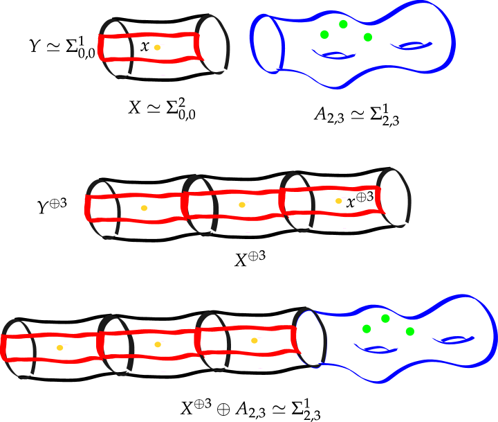
Let denote a genus topological surface with boundary components and punctures. For a topological space, we use for the configuration space parameterizing tuples of unordered distinct points on . Let , let , and let be a point in the interior of . If we think of as , we may place at . With this same identification, we denote by the rectangle . See Figure 3.
For , define the surface , which is homeomorphic to , inductively by gluing the first boundary component of along a chosen isomorphism to the boundary component of . We suggest the reader consult Figure 3 for a visualization. We denote by the -element subset of obtained as the union of the copy of the point in each of the copies of . We also let denote the complement of the interior of in and we let denote the subsurface of covered by the copies of . Again, see Figure 3 for a visualization.
Now, let denote the surface braid group. The natural map
induces a map which sends to . We note that is homeomorphic to a disc embedded in , so the fundamental group of the configuration space is just the usual Artin braid group on strands. We thus get a map of fundamental groups
or, in shorter terms, .
Remark 3.1.2.
By means of the homeomorphism between and , we may think of as the usual surface braid group on strands in a genus surface with punctures and a boundary component. We have chosen to define in this more specific way because it will help us keep track of the maps between braid groups we will need to invoke.
Remark 3.1.3.
The reason for us introducing in 3.1.1, instead of just using , is to obtain an inclusion , which gives an inclusion from a braid group for a surface with boundary component instead of from a surface with two boundary components. The key point of our homological stability results is that we will view certain systems of representations of as modules-like objects for systems of representations of , and in order to define the module structure, the inclusion is essential.
We next define coefficient systems. Our definition of coefficient systems is inspired by [RWW17, Definition 4.1], though it is not exactly the same.
Definition 3.1.4.
For a field, a coefficient system for is a sequence of vector spaces with actions so that , , and so that the action on satisfies the following condition. For any , the diagram
| (3.1) |
commutes, with maps described as follows: the right vertical map is induced by the isomorphism coming from the definition of , the left vertical map is induced by this isomorphism together with the inclusion described in 3.1.1, and the horizontal maps are induced by the given actions of on .
Remark 3.1.5.
If is a coefficient system, then naturally has the structure of a braided vector space coming from the action of a specified generator of on . For any braided vector space , the tensor powers acquire actions of satisfying (3.1). So, the definition of coefficient system for is equivalent to that of a braided vector space.
We chose to set up 3.1.4 as we did so that its structure is analogous to that of coefficient systems for higher genus surfaces, which we define next.
Definition 3.1.6.
Fix a field and let be a fixed coefficient system for . For , a coefficient system for over is a sequence of vector spaces with actions so that and the action on satisfies the following condition. For any , the diagram
| (3.2) |
commutes, with maps described as follows: the right vertical map is an equality coming from the definition of , the left vertical map is induced by the above equality and the inclusion described in 3.1.1, and the horizontal maps are induced by the given actions of on and on .
Remark 3.1.7.
It is natural to think of coefficient systems (over ) as a compatible sequence of local systems on . The compatibility condition amounts to commutativity of the diagram (3.2).
Remark 3.1.8.
Just as a braided vector space is determined by a finite amount of linear algebraic data (an endomorphism of satisfying a certain identity) it would be interesting to define a coefficient system for over in a similar way, in the spirit of the definitions introduced by Hoang in [Hoa23, §3].
We next describe coefficient systems related to Hurwitz spaces, which come from maps from to a finite group.
Example 3.1.9.
Fix . Let be a finite group and a conjugacy-closed subset of , and use notation as in 3.1.1. Choose a basepoint on . Note that acts on and hence on . Choose subsets so that and is closed under the action of on . Write for the vector space freely spanned over by the subset .
Specializing the above to the case , the action of on induces an action of on . We denote by the coefficient system for given by . This corresponds to the usual action of the Artin braid group on Nielsen tuples that underlies the classical combinatorial description of Hurwitz spaces of covers of the disc. Further, we denote by the coefficient system for over given by .
Warning 3.1.10.
We note that the cover of configuration space afforded by the coefficient system in 3.1.9 is not exactly the same thing as the space of complex points of the Hurwitz space defined in 2.4.2, but rather it is the complex points of the pointed Hurwitz space from 2.4.5. The sets carry an action of by conjugation and, via 2.4.6, the Hurwitz stack as in 2.4.2 is the quotient of the cover afforded by by this -action.
The reason we work more with this quotient is that it is easier to access from the point of view of moduli theory in algebraic geometry, while the unquotiented version is more suitable for the topological arguments we will make over the next several sections. This is easiest to see in the case , where an element of is an -tuple of elements of . Then the concatenation operation plays a key role in our arguments; but there is no well-defined concatenation on .
Example 3.1.11.
Take to be the coefficient system for with and the trivial action for all . We call the trivial coefficient system for . Let be a vector space. Then defines a coefficient system where the action of on is trivial.
Remark 3.1.12.
A different but related notion of “coefficient system” is considered in [RWW17]. Their precise definition doesn’t concern us here, but a property of the coefficient systems they consider (which they call finite degree) is that in their sequence of vector spaces , is eventually polynomial in . The coefficient system considered above, by contrast, have growing exponentially in . More precisely, the dimension grows proportionally to . In general, our coefficient systems will have dimension which is bounded by a polynomial in only when , in which case the polynomial must even be a constant polynomial.
3.2. The spectral sequence
Our next main result is 3.2.4, which sets up a spectral sequence coming from the arc complex. In order to describe this, we first describe the complex associated to a module.
Definition 3.2.1.
Let be a coefficient system for . Let , as in (4.1), which has the structure of a graded ring induced by the isomorphisms . Let be a graded module and let denote the th graded part of . Let denote the complex of graded modules whose th term is . That is, is given by
where denotes the shift by grading so that . Here we treat as living in degree for all .
To define the differential, we next introduce some notation. Using to denote the braiding automorphism of from 3.1.5, for , we let denote the automorphism , which applies to the and factors. For , we define . So, in particular, and We use to denote the multiplication map coming from the structure of as a -module. As mentioned above, we use to denote the th graded piece of a graded module , and then the differential on is given by
| (3.3) | ||||
The main case of 3.2.1 we will be interested in is when our module for is of the form , which we now define.
Notation 3.2.2.
Given a coefficient system for and a coefficient system for over , define , where here the homology denotes group homology.
In the case our coefficient system is of the form , we next describe the map concretely as well as the module structure on .
Remark 3.2.3.
In the case we take our module for in 3.2.1 to be from 3.2.2, we can describe the map concretely as follows. The inclusion from 3.1.1 coming from the inclusion induces a cup product map
This composition is . More generally, for , the inclusions from 3.1.1 give the structure of a module via the cup product map
We now describe the spectral sequence coming from the arc complex. For a picture of the page of this spectral sequence, see Figure 4. (We include the picture only in a later section as we believe it is helpful to see it side by side the proof of Theorem 4.1.1.)
Proposition 3.2.4.
Let be a coefficient system for and let be a coefficient system for over . There is a homological spectral sequence converging to in dimensions , where the th row is isomorphic to the th graded piece of . That is, is the th graded piece of for
Proof.
The proof is a fairly immediate generalization of [EVW16, Proposition 5.1]. We now fill in some of the details. One minor difference is that we opt to use an augmented version of the arc complex so that the spectral sequence converges to , instead of as in [EVW16, Proposition 5.1].
The spectral sequence will be obtained from filtering the arc complex by the dimension of its simplices. We begin by defining a combinatorial version of the arc complex, which we denote . For , let denote the subgroup obtained via the inclusion coming from 3.1.1. If , is the trivial group. Define as a set. Define the faces of the -simplex by for , where and denotes an elementary transformation moving the th point counterclockwise around the st point in . Here, . An identical computation to [EVW16, Proposition 5.3] shows for , implying is a semisimplicial set.
We next define the topological version of the arc complex, which we denote by and we define next. Choose a finite set of points in the interior of . Let denote a fixed basepoint lying on the boundary of . Following Hatcher and Wahl [HW10, §7], we define a complex as follows. A vertex of is an embedded arc in with one endpoint at and the other at some . For , a -simplex of is a collection of such arcs, which are disjoint away from . In particular, there are no simplices of dimension larger than . Note that if we omit the simplex, and only consider , the resulting complex is the complex denoted in [HW10, §7], with , , and Hatcher and Wahl prove in [HW10, Proposition 7.2] that is -connected. (Recall is -connected if for .) Since the skeleton of is a point and is -connected, both of these spaces have trivial homotopy groups in degree and so the resulting boundary map yields a homotopy equivalence of spaces in degrees . We will soon construct a simplicial chain complex associated to , and the above implies it has trivial homology in degrees .
We now relate the two models and of the arc complex. In [EVW16, Proposition 5.6] a natural map , identifying these semisimplicial sets, was constructed when , and this readily generalizes to the case of arbitrary and .
We next describe the claimed spectral sequence. As in [EVW16, p. 757], for a space with a action, we write for the quotient, also known as the Borel construction . We will write to denote the free vector space on the simplices of , which is a representation. Then, because is an equivalence of -connected spaces, the map
is an isomorphism in degrees . That is, the left cohomology group vanishes for . We can also identify with via the isomorphisms
Filtering by the simplicial structure on , we obtain a spectral sequence
| (3.4) |
Since is -connected, has trivial homology in degrees and hence the right hand side of (3.4) vanishes for . Analogously to [EVW16, Lemma 5.4], one may verify that the differential is identified with the th graded part of the differential as in (3.3). The spectral sequence we have now constructed has bounds . Replacing by gives and yields the vanishing in degrees , or equivalently . This gives desired spectral sequence, as in the statement. ∎
4. Deducing homological stability results for coefficient systems
In this section, we prove that certain types of coefficient systems have nice homological stability properties, following closely ideas from [EVW16]. In § 4.1 we give a general formulation of this stability property. In § 4.2 we show that finitely generated modules for coefficient systems with a suitable central element satisfy this stability property. Finally, in § 4.3 we put together all the topological material developed in this section and the previous one to arrive at an exponential bound on the cohomology of these coefficient systems.
For the reader primarily interested in our application to Selmer groups, only two results from this section needed in future parts. First, 4.3.4 will be used as a central ingredient in the proof of 8.2.3. Second, Theorem 4.2.2 will be used in the proof of Theorem A.5.1 to show the trace of Frobenius on the cohomology stabilizes.
4.1. Homological stability for -controlled coefficient systems
We next prove the main homological stability result of this paper in Theorem 4.1.1, using the arc complex spectral sequence from the previous section. To set things up in a general context, we define the notion of a -controlled coefficient system. For an object in a category with a grading, we define to be the supremum of all such that . Note that has a grading by the number of points , and hence the same is true for . The idea is that modules for -controlled coefficient systems have degrees of their th homologies controlled in terms of degrees of their th and st homologies. For a graded ring, we say an element is homogeneous if it lies in a single degree of the grading of .
Definition 4.1.1.
Define
| (4.1) |
The monoidal structure of supplies with the structure of a graded ring supported in nonnegative gradings. Fix a homogeneous element of positive degree so that left multiplication by induces a map . A coefficient system for is -controlled if and are finite and there exists a constant so that for any left -module , the following two properties hold:
-
(1)
We have
-
(2)
The map induced by left multiplication by , denoted , induces an isomorphism for
Next, we give a crucial example of a -controlled coefficient system.
Example 4.1.2.
Let be a group and be a conjugacy class in . We will assume is non-splitting in the sense of [EVW16, Definition 3.1], meaning that generates and for every subgroup , either consists of a single conjugacy class in or is empty. Let , as defined in 3.1.9. As described in [EVW16, §3.3], the ring is generated in degree by elements of the form (corresponding to right multiplication by ) for . Consider the map , where denotes the order of . We will show in A.3.1, that both have finite degree. This is -controlled precisely by [EVW16, Theorem 4.2]. Note that the ring is called in [EVW16, Theorem 4.2].
The proof of this next result closely follows the proof of [EVW16, Theorem 6.1].
Theorem 4.1.1.
Suppose is a -controlled coefficient system for and is a coefficient system for over . Using notation as in 3.2.2, assume moreover that and are finite. Then, there exist constants depending on and but not on or so that restricts to an isomorphism whenever .
Proof.
By way of induction on , we will prove there exist nonnegative constants and , independent of and , so that
| (4.2) |
for all . Once we establish (4.2), we will obtain the result because, plugging in the cases and , we get
Hence, by 4.1.1(2), we find restricts to an isomorphism whenever
and we can then take the constant and .
We next assume the result holds for , and aim to show it holds for . It suffices to show
| (4.3) | ||||
as then 4.1.1(1), implies
which is the inductive claim we wished to prove.
We conclude by proving (4.3). From 3.2.4, we can identify . Therefore, it is enough to show in degree . The differential coming into comes from , see Figure 4. By our inductive hypothesis, these vanish in degree . When is either or , we can bound
Hence, once the degree satisfies , we find for either or . Finally, so long as , for the degree, by 3.2.4. Once we verify and , we will conclude . In particular, since we have assumed , and holds by from 4.1.1, we find , and so (4.3) holds so long as . ∎
4.2. A sufficient condition for homological stability
We next set out to show that a wide variety of and satisfy the hypotheses of Theorem 4.1.1. We establish this in Theorem 4.2.2. For the purposes of this paper, our generalization of [EVW16, Theorem 4.2] given in Theorem 4.2.1 is not necessary, as we will only need to apply this to coming from Hurwitz stacks, which is already proven in [EVW16, Theorem 4.2] applies. However, we include this generalization as we believe it may be useful for approaching similar homological stability problems in the future.
To start, we give a sufficient criterion for a ring to be -controlled in terms of a central operator . The following is the above mentioned generalization of [EVW16, Theorem 4.2].
Theorem 4.2.1.
Suppose is a coefficient system for and define as in (4.1). Suppose is a homogeneous positive degree central element such that and are both finite. Then, is -controlled.
Proof.
This is essentially proved in [EVW16, Theorem 4.2]. While technically the ring used there is for a specific , the proof generalizes to the case stated here, as we now explain. Throughout the proof of [EVW16, Theorem 4.2], one may replace with , and, for an module, one may then use our definition of from 3.2.1 in place of the definition in [EVW16, §4.1]. The two parts of the proof of [EVW16, Theorem 4.2] whose generalization requires some thought are the content of [EVW16, p. 755], where one wishes to establish the bound , as well as [EVW16, Lemma 4.11]. Both of these refer to specific elements of the ring in [EVW16], which is related to Hurwitz stacks.
The only step of [EVW16, p. 755] where one cannot easily replace elements of with elements of is in the third to last paragraph. To explain why this still holds, let denote the map sending , where denotes the class of in , and denotes the multiplication using that is an module. For , we similarly use to denote the product of the class of in with . To establish the third to last paragraph of [EVW16, p. 755], we wish to verify that the composite map
vanishes. For , if denotes the isomorphism giving the structure of a braided vector space, corresponding to a generator of , we obtain that . This is equal to because as elements of : Indeed, a generator of acts via on , so taking coinvariants via identifies and .
Lemma 4.2.1.
For a coefficient system, the action of on is .
Proof.
We generalize the proof of the analogous statement given in [EVW16, Lemma 4.11]. Start with some element . Define the linear operator
with notation as follows: we use notation as in 3.2.1, we use to denote a lift of from to , and, for we use for the image in . First, we need to verify this map is independent of the choice of lift of . If we chose a different lift , we can write for some . Writing as a product of generators, we may assume . Now, for and , define as the inclusion sending strands of to strands in the range . More formally, this can be realized in terms of 3.1.1 as the inclusion
where the first map is the inclusion to the second component, the second map is the product of with the map of braid groups associated to the inclusion , and the third map is the map of braid groups associated to the inclusion . The well definedness of follows from the identity
applied to , as the above computation shows this maps to the same element as since their images in are related by .
Since is generated in degree , it is enough to prove right multiplication by nullhomotopic. Having shown that is well defined, we now compute
which shows right multiplication by is nullhomotopic. ∎
We next observe that is noetherian. A similar argument in the context of Hurwitz stacks was given in [DS23, Proposition 3.31] and also [BM23, Lemma 3.3].
Lemma 4.2.2.
Let be a coefficient system for . Suppose has some homogeneous positive degree so that is finite. Then is noetherian.
Proof.
Note that is not commutative. However, we claim is a finite module over a commutative finitely generated ring, hence noetherian. Let denote the commutative subring generated by over . We claim is a finite module over . We will in fact show that is generated over by all elements of degree at most . Since each is finite dimensional, this will imply that is finitely generated over . To prove our claim, by induction on the homogeneous degree of an element, it is enough to show that any homogeneous element with can be written in the form for and . Indeed, consider the image . Because has finite degree, there is some element of degree at most so that . This implies for some , and hence with and . ∎
Using noetherianness of , we can also prove the other hypotheses of Theorem 4.1.1 hold for finitely generated modules.
Lemma 4.2.3.
Let be a coefficient system for . Suppose has some homogeneous positive degree central so that and are both finite. Then, if is a finitely generated module over , both and have finite degree.
Proof.
First, since is generated in degree , , and this quotient is supported in the degrees of generators of over . Therefore, is finitely generated, with each generator having degree at most , if and only if .
Next, we show is finite. Since , there is a spectral sequence . By the low degree terms exact sequence coming from the spectral sequence, in order to bound , it is enough to bound and . By Theorem 4.2.1, and have finite degree. In particular, they are finite modules. Hence it suffices to show and are finite. By noetherianness of , as established in 4.2.2, we may choose a free resolution of the finite module of the form where each term is a finite free module, hence of finite degree. Applying to this resolution and taking cohomology shows that has finite degree for all . ∎
We next show that in the case , the finite generation hypothesis of 4.2.3 is automatic.
Lemma 4.2.4.
Suppose is a coefficient system for . If is a coefficient system for over , then is finitely generated as a module.
Proof.
We may view as an module via 3.2.3. Via the inclusion from 3.1.1, there is a surjection . We therefore obtain a surjection of graded modules
Hence, it is enough to show is finitely generated as an module. Indeed, since acts trivially on ,
and so the desired finite generation holds because is a finite dimensional vector space. ∎
Combining our work above, we obtain that if we have coefficient systems and , and has a central homogeneous element of positive degree with finite degree kernel and cokernel, then Theorem 4.1.1 applies.
Theorem 4.2.2.
Suppose is a coefficient system for and is a homogeneous central element of positive degree such that and are both finite. If is a coefficient system for over , then there exist constants and independent of and so that induces an isomorphism whenever .
Proof.
This follows from Theorem 4.1.1, once we verify its hypotheses. We find is -controlled by Theorem 4.2.1. From 4.2.4, is finitely generated as an module. By 4.2.3, it follows that and both have finite degree. ∎
Remark 4.2.5.
Via private communication with Oscar Randal-Williams, it seems likely that one may be able to prove Theorem 4.2.2 using a setup similar to that in [RW20]. However, this is by no means obvious, and we believe it would be very interesting to work out the details. In particular, one of the trickiest parts to generalize is [RW20, Proposition 8.1] where it is used that . In our setting we need to instead analyze , for a suitable value of in place of .
4.3. An exponential bound on the cohomology
Our main application of the above homological stability results to the BKLPR heuristics comes from the bound on cohomology in 4.3.3, and the corresponding consequence 4.3.4. There are two inputs. The first is our above homological stability results. The other is a bound on the CW structure of configuration space.
We now give this second bound, which nearly appears in [BS23, §4.2] in the case that . We now give the straightforward generalization to the case of arbitrary . We will be brief here, but encourage the reader to consult [BS23, §4.2] for further details. We thank Andrea Bianchi for suggesting the following approach.
Lemma 4.3.1.
For , the space , parameterizing unordered points in the interior of , has -point compactification with a cell decomposition possessing at most cells.
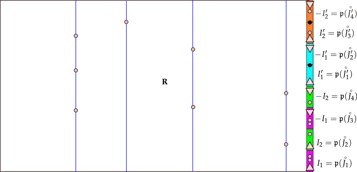
Proof.
The idea is to generalize the construction of [BS23, §4.2] to the case that as follows. We modify their setup so that the right edge of their rectangle includes the intervals , as in the case , and then additionally includes the intervals from bottom to top, see Figure 5.
We now spell this out in some more detail, reviewing the notation of [BS23, §4.2]. First, we describe as a quotient in a particular way, which will be useful for describing a cellular structure on the one point compactification of its configuration space. Let be a rectangle. Decompose the side into consecutive intervals of equal length ordered and oriented with increasing second coordinate, as in Figure 5. Let be the set of the points consisting of the larger endpoint of for . Let denote the punctured rectangle where we remove . Let denote the quotient of obtained by identifying with , with , and with via their unique orientation reversing isometry for and . Let denote the quotient map. Then, is homeomorphic to .
We next give a description of the cellular structure of . Throughout, for a topological space, we will use to denote the interior of .
-
(1)
The space has a single cell , which is the image of any of the endpoints of the , and is also identified with the larger endpoint of .
-
(2)
The space has one-cells, described as follows. There are the -cells , where with and . There are the -cells for . Finally, there is .
-
(3)
Finally, has one -cell which is
We let denote the composition of with the linear map sending for . We let denote the composition of with the linear map sending for . (This notation differs from that of [BS23, §4.2], but it is slightly more convenient for our purposes.)
We next introduce notation to define the cells in the CW complex we will construct. For , an -tuple, which we denote by , consists of
-
(1)
an integer
-
(2)
a sequence of positive integers
-
(3)
a sequence of non-negative integers
-
(4)
a sequence of non-negative integers
such that . The above data will index ways to split up points, representing a point of , into different cells of .
We next define the cells determining a CW structure for the one point compactification of . We write and use the notation for our surface described above. For an -tuple, let denote the subset of (which we recall parameterizes points in the interior of ) which satisfies the following conditions.
-
(1)
For , points lie on .
-
(2)
For , points lie in .
-
(3)
There are exactly real numbers such that admits at least on point in having as a coordinate.
-
(4)
For all , exactly points of which lie in have first coordinate equal to .
Each lies in a unique subspace . Given an -tuple , the space is homeomorphic to an open disc. Let denote the dimension of this disc. Let denote the standard -dimensional simplex. Define . Using to denote the -point compactification, for an -tuple, define the map given in simplicial coordinates by
where denotes the superposition product. The map restricts to a homeomorphism sending the and the boundary to the union of and some of the subspaces where .
As in [BS23, Proposition 4.4], one may verify the together with form a cell decomposition for the one point compactification of .
Finally, we bound the number of cells in this structure by . Note that the number of cells is the same as the number of -tuples . A cell can equivalently be described by a choice of , and a collection of non-negative integers summing to . By “stars and bars,” such collections of integers are in bijection with subsets of of size . Varying over different possible values of yields that the total number of cells is equal to the number of subsets of of size at least . This is at most the number of subsets of , which is , as we wished to show. ∎
As an easy consequence of the above bound on the number of cells, we obtain the following bound on homology.
Lemma 4.3.2.
Suppose is a coefficient system for and is a coefficient system for over . Then,
Proof.
Since , the representation of corresponds to a local system on If denotes the -point compactification and , denotes the inclusion, we have an isomorphism between the compactly supported cohomology and the relative cohomology
| (4.4) |
We will now bound the dimension of this relative cohomology group. We will use the cell structure on from 4.3.1 which has at most cells. The cellular cochain complex which computes the th cohomology group (4.4) has dimension less than . It follows from Poincaré duality that
Combining our homological stability results with the above bounds on homology gives the following bound on cohomology. For the following, we continue to use notation from 3.2.2.
Proposition 4.3.3.
Let be a prime. Suppose is a -controlled coefficient system for and is a coefficient system for over . Assume moreover that and are finite. Then, there is a constant depending on , and the sequence , but not on the subscript or the index so that
| (4.5) |
for all .
Proof.
Since the dimensions of the vector spaces in (4.5) are finite, and we are working with representations over a field, it follows from the universal coefficient theorem that . Hence, it is enough to bound By Theorem 4.1.1, there are constants and so that whenever Therefore, applying this repeatedly, it is enough to show for any . By 4.3.2, . Hence, we only need to produce some constant so that
We may assume , as otherwise and the statement is trivial. Because ,
The claim then follows by taking
We now reformulate the above in a slightly more convenient form for our applications.
Corollary 4.3.4.
Suppose is a -controlled coefficient system for and is a coefficient system for over . Assume that there is a central homogeneous positive degree element such that and are both finite. Suppose assume corresponds to a local system on via the identification with for some finite étale cover of spaces over the complex numbers. Then, there is a constant depending on the sequence but not on the subscript or index so that
for all .
Proof.
This is an immediate consequence of 4.3.3, upon identifying group cohomology for a finite group with cohomology of the corresponding finite covering space, once we verify that is -controlled and and are finite. We have that is -controlled by Theorem 4.2.1. From 4.2.4, we find that is finitely generated as an module. By 4.2.3, we find and both have finite degree. ∎
5. The Selmer stack and its basic properties
In this section, we set up the Selmer stack, which is a finite cover of the stack of quadratic twists of an abelian variety that parameterizes pairs of a quadratic twist and a Selmer element for that quadratic twist. We first define the Selmer stack in § 5.1. In § 5.3 we prove basic properties of the Selmer stack, such as the fact that it is a finite étale cover of the stack of quadratic twists. Since the definition given in § 5.1 is not obviously connected to Selmer groups, in § 5.3 we relate the Selmer stack to Selmer groups. Variants of the Selmer stack for the universal family were studied in [Lan21] and [FLR23], and many of the proofs in this section follow ideas from those articles.
5.1. Definition of the Selmer stack
We now set up notation to define the Selmer stack.
Definition 5.1.1.
Let be a Deligne-Mumford stack and a positive integer. A locally constant constructible sheaf of free modules on is symplectically self-dual if there is an isomorphism so that the resulting pairing factors through .
Remark 5.1.2.
Sometimes, a symplectically self-dual sheaf is called a weight symplectically self-dual sheaf. Since this is the only kind of symplectically self-dual sheaf we will encounter in our paper, so we omit the “weight ” adjective. All symplectically self-dual sheaves we encounter will be assumed lcc sheaves of free modules.
Example 5.1.3.
An important example of a symplectically self-dual sheaf for us will be , where is an abelian scheme as in 2.4.1 with a polarization of degree prime to , for invertible on .
Notation 5.1.4.
Keep notation for as in 2.4.1. Let be a tame symplectically self-dual sheaf on .
In order to define a Hurwitz stack for the group , let denote the subset sending loops around the geometric points in the degree divisor to the trivial element of and loops around the marked points (corresponding to geometric points of the divisor ) to the nontrivial element of . (Since is abelian, this Hurwitz stack is a gerbe over its coarse space.) Define to be .
We will assume throughout is even, as otherwise there are no such covers by Riemann-Hurwitz. Informally, is a moduli space for finite double covers of ramified over a degree divisor , disjoint from . Let denote the composite projection and let denote the universal proper curve. The universal open curve possesses a natural finite étale double cover , which is branched precisely along the boundary divisor (but not along the preimage of ).
Define . This is a sheaf on whose fiber over is a sheaf on which is the quadratic twist of over along the finite étale double cover corresponding to the surjection , which is branched over .
With the above notation in hand, we are now prepared to define the Selmer stack.
Definition 5.1.5.
Maintain notation as in 5.1.4 and let be a positive integer. We assume is invertible on . As in 5.1.4, we have a symplectically self-dual sheaf on , which we are assuming is an lcc sheaf of free modules. This gives rise to a symplectically self dual sheaf on and maps
Define the Selmer sheaf of log-height associated to over to be . The Selmer stack, , is the algebraic stack representing this étale sheaf.
Remark 5.1.6.
For odd , the Selmer stack is never a scheme because is a gerbe over a scheme, and is an odd degree cover of . Fortunately, since this is a gerbe, its stackiness is rather mild. This will pose some technical, yet overcomable, obstacles.
We next give a couple examples of types of symplectically self-dual sheaves coming from abelian varieties, which will be important for our applications to the BKLPR heuristics.
Example 5.1.7.
Suppose is a polarized abelian scheme with polarization of degree prime to over . Take . Note , since the polarization has degree prime to . Then, the Weil pairing gives the structure of a symplectically self-dual sheaf on . Further, with notation as in 5.1.4, defines a sheaf on . An important example of a Selmer sheaf for us will be .
Example 5.1.8.
A slightly more general setup than 5.1.7 is the following. Suppose we are in the setting of 5.1.4, and is a closed point. Suppose we are given a symplectically self-dual sheaf over so that the fiber over defines a sheaf which is of the form for a polarized abelian scheme with polarization degree prime to . Then we obtain a Selmer sheaf over so that . The difference between this and 5.1.7 is that we may not have any abelian scheme over restricting to over .
Remark 5.1.9.
In fact, the 5.1.8 will be the setting we work in to prove our main result Theorem 1.1.2 because it is relatively easy to lift symplectically self-dual sheaves from the closed point of a DVR to the whole DVR, as we explain in 10.2.2. However, we are unsure whether it is possible to lift abelian schemes in our setting.
We conclude this subsection with some notation recording data associated to a quadratic twist, which we will use throughout the paper.
Notation 5.1.10.
With notation as in 5.1.4, for a point or geometric point, let denote the image of under the map . We use to denote the fiber of over , to denote the fiber of over , and we use to denote the fiber of over the point .
Assume we are further in the setup of 5.1.7 or 5.1.8 and . We use to denote the fiber of the abelian scheme over , where and denote the pullback along and , and denotes the Weil restriction along . Note that is an abelian scheme over . We use to denote the Néron model over of . We let denote the divisor associated to , the image of under the projection .
5.2. Basic properties of the Selmer stack
We next develop some basic properties of the Selmer stack. The next lemma shows the Selmer sheaf commutes with base change. The proof is similar to [FLR23, Lemma 2.6], though some additional technical difficulties come up related to working over the space of quadratic twists, instead of the universal family.
Lemma 5.2.1.
Use notation as in 5.1.4. In particular, is a tame symplectically self-dual sheaf. Suppose invertible on . Then, the sheaf is locally constant constructible and its formation commutes with base change on . Further, for , both and are locally constant constructible for all and their formation commutes with base change on .
Proof.
In order to prove the result, we first set some notation. We have a natural map obtained from the map and the definition [FK88, I.8.6]. Similarly, we have a map obtained from the composition of functors spectral sequence for . Note that is injective by the Leray spectral sequence.
Our first goal is to show is the image of . Since is injective, it only remains to show is surjective. Because is an isomorphism over , is supported on , which is finite over , we find This implies is surjective and so is a constructible sheaf.
We conclude by showing and are both locally constant constructible, and their formation commutes with base change. This will imply is locally constant constructible and its formation commutes with base change, as it is the image of the map .
We first show is locally constant constructible in the case that is prime. Note that its formation commutes with base change by proper base change for any . Using [Lau81, Corollaire 2.1.2 and Remarque 2.1.3], it is enough to show the Swan conductor of is constant. As in [Lau81, Remarque 2.1.3], the Swan conductor over a point is a sum of local contributions, one for each geometric point of and one for each geometric point of over the image of in . At each geometric point of , because we are taking a quadratic twist along , the ramification index is , and hence the ramification is tame, since is invertible on . We are also assuming the ramification along points of is tame for . This is identified with the corresponding ramification for along points of , and hence this is tame as well. Therefore, the Swan conductor vanishes identically.
Next, we show is locally constant constructible for every positive integer as in the statement of the lemma, using the case that is prime, settled above. As an initial step, we may reduce to the case is a prime power by observing that if has prime factorization then . Now, suppose is a prime power, and inductively assume we have proven is locally constant constructible for all . Since and is a locally constant constructible sheaf of free modules, we have an exact sequence
Applying to the above sequence, we get a long exact sequence on cohomology
Since all but the middle term are locally constant constructible by our inductive assumption, it follows that is also locally constant constructible by [Sta, Tag 093U].
We conclude by showing is locally constant constructible and its formation commutes with base change. Since is locally constant constructible, it follows from Poincaré duality [Ver67, Theorem 4.8] and the isomorphism coming from the polarization of degree prime to that
Taking gives . Since we have seen is locally constant constructible and its formation commutes with base change, the same holds for . ∎
Notation 5.2.2.
Let be a field and let be a smooth proper geometrically connected curve over of genus , with an open subscheme. Let an abelian scheme over with Néron model . Let denote the identity component of the Néron model , meaning that is the open subscheme of so that each fiber is nonempty, connected, and contains the identity section, see [BLR90, p. 154]. Let denote the component group of the Néron model of . We use to denote the geometric component group.
The following proof is quite similar to [Lan21, Lemma 3.21]. We thank Tony Feng for suggesting the idea that appeared there for bootstrap from the prime case to the general case, which we reuse here. In the next lemma, note that since we are working over an algebraically closed field, the component group is the same as the geometric component group.
Lemma 5.2.3.
Let be an algebraically closed field, let be a smooth proper geometrically connected curve over of genus . Let be a symplectically self-dual lcc sheaf of free modules on an open . Suppose that
-
(1)
for each prime , , and , the multiplication by map is surjective.
-
(2)
.
Then is a free module. In the case is of the form of , for an abelian scheme, hypothesis above is satisfied if the geometric component group has order prime to .
Proof.
Using the Chinese remainder theorem, we can reduce to the case that is a prime power. Suppose We will show by induction on that
For we claim there is an exact sequence
| (5.1) |
This is left exact because the analogous sequence for in place of is left exact. This sequence is right exact by assumption (1) from the statement of the lemma.
We now prove the final clause of the statement of the lemma: In the case , the cokernel of the map is identified with . This is trivial by assumption as . Therefore, in this case, holds.
We next claim . The former holds by assumption . By [Mil80, V Proposition 2.2(b)] and the polarization , we find
The long exact sequence associated to (5.1) and the vanishing of the th and nd cohomology above implies we obtain an exact sequence
| (5.2) |
Induction on implies and we wish to show is free of rank . By the structure theorem for finite abelian groups, it suffices to show the kernel of multiplication by on has order . The multiplication by map factors as . We know from (5.1) that is injective so
which has size , as we wished to show. ∎
We next aim to compute a formula for the rank of the Selmer sheaf, in favorable situations, in 5.2.6. First, we introduce notation needed to state that formula.
Definition 5.2.4.
Suppose is a prime number. Given a locally constant constructible sheaf of free modules on an open of a curve , for any point , there is an associated action of the inertia group at on the geometric generic fiber of , which is well defined up to conjugacy. We use to denote the corank of the invariants of , i.e., . In general, if is not necessarily a prime number, for each prime we use , and if is independent of , we denote this common value simply by . Whenever we use the notation in the case has multiple prime divisors, we are implicitly claiming it is independent of the prime divisor.
Example 5.2.5.
If is prime, and , then for any , if and only if inertia acts trivially at , i.e., extends over the point . If is a relative elliptic curve and the order of the geometric component group of the Néron model of at is prime to , then whenever has multiplicative reduction at and whenever has additive reduction at .
Proposition 5.2.6.
Maintain notation as in 5.1.4, so, in particular, is a tame symplectically self-dual lcc sheaf of free modules. Suppose is odd and . Assume that is the spectrum of an algebraically closed field. Assume that
-
(1)
for each prime , each integer with , and each integer , the multiplication by map is surjective
-
(3)
the sheaf is irreducible for each prime .
Assume is invertible on . For each , consider the following three properties.
-
(1’)
for each prime with and , the multiplication by map is surjective
-
(2’)
-
(3’)
the sheaf is irreducible for each prime .
Then, always holds, holds if holds, and holds if holds.
Moreover, assuming and , the map is finite étale, representing a locally constant constructible sheaf of rank free modules, whose formation commutes with base change.
Proof.
First, observe that by 5.2.1, is finite étale, corresponding to a locally constant sheaf of modules, and its formation commutes with base change on .
We now verify that condition hold for quadratic twists of , ramified over a divisor disjoint from , using condition . If corresponds to a representation of , the quadratic twist corresponds to tensoring this representation with an order character, whose local inertia at any point outside of is trivial. Surjectivity of the map from can only fail at points . If , since surjectivity can be verified locally, surjectivity for at follows from the corresponding surjectivity for at . If , the stalk of is trivial, as it is identified with the invariants of multiplication by , which is trivial, and so surjectivity at such points is automatic.
Next, we check holds, just using . We wish to show . Thinking of as a representation of , a section corresponds to an invariant vector. However, since , local inertia at a point of acts by , and so there are no invariant vectors.
Third, we show holds for , assuming holds for . Note that the quadratic twist of the sheaf is obtained by tensoring the corresponding representation of with a character. This preserves irreducibility.
We next show this corresponds to a sheaf of free modules. We may check this at any point of since the formation of commutes with base change on by 5.2.1. It follows that over a geometric point of , the hypotheses and of 5.2.3, which follow from and in the statement of this proposition, are satisfied for any quadratic twist of . Therefore, corresponds to a sheaf of free modules by 5.2.3.
Finally, we compute the rank of this sheaf. Since we have shown is an irreducible locally constant constructible sheaf on , we can compute the formula for its rank after reduction modulo any prime , and hence assume that is prime. The formula for the rank is given in [Kat02, Lemma 5.1.3]. Technically, the argument is given there for lisse sheaves, but the same computation applies to sheaves. In particular, with the above assumptions, if , for an algebraically closed field, has rank . ∎
5.3. Connecting points of the Selmer stack and Selmer groups
The next two lemmas connect the Selmer stack to the sizes of Selmer groups and their proofs are quite similar to [Lan21, Proposition 3.23] and [Lan21, Corollary 3.24] respectively.
Lemma 5.3.1.
Proof.
Using 5.2.1, we know the formation of the Selmer sheaf commutes with base change, and hence for a geometric point over , the geometric fiber of over is identified with
To distinguish between étale and group cohomology, we use denote group cohomology and to denote étale cohomology. Let . The points of are the invariants of . That is, .
We relate this group to using the Leray spectral sequence
| (5.3) |
When , we want to show is an isomorphism, so it suffices to show . This holds using 5.2.6(3’). ∎
Lemma 5.3.2.
With the same assumptions as in 5.3.1, let , and use to denote the Selmer group of the generic fiber of over . We have
6. Identifying Selmer elements via Hurwitz stacks
Throughout this section, we’ll work over the complex numbers . One of the main new ideas in this article is that Selmer elements can actually be parameterized by a Hurwitz stack. The reason for doing this is that the topological methods of the first part of the paper can, as in [EVW16], be used to control the number of -points on certain Hurwitz stacks. Using the identification between Selmer stacks and Hurwitz stacks, we will thus be able to count -points on Selmer stacks. These counts underlie our main theorems.
We produce an isomorphism from the Selmer stack to a certain Hurwitz stack over the complex numbers parameterizing covers of our base curve over . This is shown in 6.4.5. Before jumping into the details, we describe the idea of this isomorphism in § 6.1. Continuing to the proof, we give a monodromy theoretic description of torsion sheaves in § 6.2, and give a monodromy theoretic description of torsors for torsion sheaves in § 6.3. Finally, we identify the Selmer stack with certain Hurwitz stacks in § 6.4.
6.1. Idea of the isomorphism
We will now describe the idea of the proof in the context of torsion in abelian varieties, though below the proof is carried out in the more general context of symplectically self-dual sheaves. The basic idea is that Selmer elements for an abelian variety over of relative dimension with Néron model over correspond to torsors for . We can identify with a Galois cover of via its Galois representation. We can then identify torsors for as covers of , see 6.3.2. This roughly corresponds to the fact that a torsor for can translate the monodromy of by an element of a geometric fiber of , which can be identified with . The bulk of this section amounts to working out the precise conditions on the monodromy of these Hurwitz stacks.
6.2. Symplectically self-dual sheaves in terms of monodromy
Recall that throughout this section, we are working over . As in 2.4.1, we begin with a smooth projective connected curve over , and a nonempty open subscheme . For a divisor, we work with a sympletically self-dual sheaf over of rank . A useful example to keep in mind will be when we are in the setting of 5.1.8 and there is an abelian scheme and . The main application will occur when is a quadratic twist of a sheaf , ramified over .
We now describe in terms of its monodromy. Fix a basepoint and choose an identification . Because the fundamental group acts linearly on , we obtain a map . Because the sheaf is symplectically self-dual, and we are working over where the cyclotomic character acts trivially, this representation factors through . In other words, we obtain a monodromy representation
| (6.1) |
For convenience of notation, label the points of by . As in Figure 6, we can draw oriented loops based at which pairwise intersect only at so that
-
(1)
forms a basis for ,
-
(2)
is a loop winding once around corresponding to the local inertia at , where are the points in , and
-
(3)
is a loop winding once around corresponding to the local inertia at .
The above loops form generators of and satisfy the single relation
| (6.2) |
Since is a local system on , the monodromy representation determines .
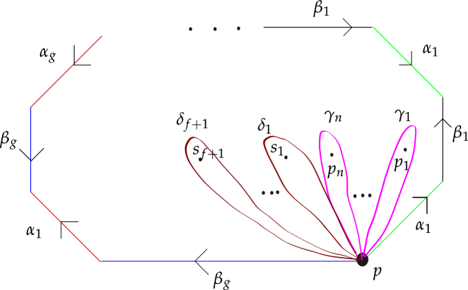
6.3. Torsors for symplectically self-dual sheaves in terms of monodromy
The next result we are aiming toward is 6.3.7, which gives a description of torsors.
We retain notation from § 6.2. For a divisor, we use to denote the inclusion. As a first observation, we show that any torsor for over is determined by its restriction to .
Lemma 6.3.1.
The restriction map is injective. Its image consists of those torsors such that for each , there is some sufficiently small complex analytic open neighborhood such that is the restriction of a torsor to .
Proof.
In the étale topology, the spectral sequence associated to the composition yields the injection . Using the comparison between étale and complex analytic sheaf cohomology [SGA72, Exposé XI, Théoréme 4.4(iii)] we may describe elements of as torsors in the complex analytic topology for . The condition that a torsor lies in the image of is precisely the condition that it extends to an torsor over a sufficiently small neighborhood of each point . ∎
Recall our goal is to give a monodromy theoretic description of torsors. Using 6.3.1, we can describe torsors as torsors which extend over a small neighborhood of each and . We next describe torsors, and then, in 6.3.6, give the condition that such a torsor extends over . First, we introduce notation used to describe the monodromy representation parameterizing torsors.
Definition 6.3.2.
The affine symplectic group is where the action of on is via the standard action of matrices on their underlying free rank module of rank .
Remark 6.3.3.
By definition, sits in an exact sequence
| (6.3) |
with inclusion map and quotient map . With this presentation, can be explicitly described as those matrices of the form
|
Notation 6.3.4.
Suppose is a finite module of the form . Define , with acting via reduction modulo and the standard representation on each factor . In particular, sits in a split exact sequence
| (6.6) |
We next describe the condition for a torsor for to extend over a puncture, in terms of monodromy. By § 6.2, can be described in terms of , which has target . A torsor for can be described in terms of together with the additional data of transition functions lying in . In total, can be described in terms of a monodromy representation
A composition of loops in maps under to the product of their corresponding matrices, viewed as elements of via (6.4).
Remark 6.3.5.
By construction, for as defined in (6.3), .
We now describe the condition that a torsor extends to a torsor. We note, first of all, that by 6.3.1, we know that this condition only depends on the restriction of to local inertia groups. Since these inertia groups are procyclic, this amounts to specifying some subset of , necessarily closed under conjugacy, in which the local monodromy groups are constrained to lie. In the following proposition, we work out what these constraints look like in explicit matrix form.
Lemma 6.3.6.
With notation as in § 6.2, let denote the inclusion. Suppose with a small loop around whose image under corresponds to the local inertia at . Let so that, after choosing a suitable basis , we may write in the form
Under the identification of as in (6.4), we can extend a torsor to an torsor in some complex analytic neighborhood of if and only if
| (6.7) |
for some vector . Stated more intrinsically, we can extend to a torsor if and only if the vector in (6.4) lies in
Proof.
First, 6.3.5 shows all entries of the matrix in (6.7) are necessary and sufficient for to extend to a torsor except the first entries of the last column, accounting for the and the .
Choose a simply connected neighborhood of and fix a basepoint . To conclude the proof, we will show the claimed entries in the last column of (6.7) from rows to are if and only if extends to a torsor over . We start by assuming the torsor extends, and aim to show the entries mentioned above are . Note that we can identify as a subsheaf which restricts to as the inertia invariants. Therefore, any torsor has a distinguished subtorsor, which is given as . Since is simply connected, this torsor is trivial, which implies that the local inertia at acts trivially on , and hence there is a in (6.7) as claimed.
Conversely, suppose there is a in the second row of the third column of (6.7). We will conclude by showing the torsor extends over . We obtain a section of over corresponding to each element of , and hence a subsheaf . By gluing to along , we obtain an torsor , which is the desired extension of . ∎
We can now describe torsors in terms of monodromy data.
Lemma 6.3.7.
With notation as in § 6.2, let be an irreducible symplectically self-dual sheaf on . Suppose . Fix some quadratic twist of , ramified along a degree divisor , in the sense that is some fiber of , so that we obtain a corresponding monodromy representation . Suppose satisfies the hypotheses and of 5.2.6. There are precisely isomorphism classes of torsors for , which can be described in terms of monodromy data by specifying a representation up to conjugacy, satisfying the following conditions:
-
(1)
The image of under is of the form (6.4) with .
-
(2)
If , the image of under is conjugate to a matrix of the form (6.7), where we take there to be here.
-
(3)
We have .
Let denote the inclusion. As mentioned above, we consider two torsors and equivalent if there is some so that for every , with as in (6.3).
Proof.
Using 6.3.1, we can describe torsors for as torsors for which extend over a neighborhood of each . By 6.3.5, condition precisely corresponds to the condition that the associated local system associated to on is that associated to , and hence is a torsor. By 6.3.6, an torsor extend to a torsor over , if and only condition holds, and extends over if and only if condition holds. We consider the representations up to conjugacy, as this corresponds to a change of basepoint of , and expresses the usual condition for two torsors to be equivalent.
To conclude, we wish to see that there are isomorphism classes of torsors specified by the above data. Indeed, we see there are possible values can take on the loops in order to satisfy . For each , there are possible values of , because . For each , there are possible values of . We additionally must impose the condition that , from the relation (6.2) defining the fundamental group, and that we consider these torsors up to conjugacy. Before imposing these two conditions, there are possible tuples of matrices. The first condition imposes independent constraints on the matrices. Further, the conjugation action always identifies elements since the representation is center free, using that it is irreducible and that contains no scalars, other than . Altogether, this yields such torsors. ∎
6.4. Identifying Selmer stacks with Hurwitz stacks
We will use the above description of torsors to identify the Selmer stack with a certain Hurwitz stack in 6.4.5. We next define that Hurwitz stack.
Notation 6.4.1.
Let . Given a symplectically self-dual sheaf over as in 5.1.4, and fixing values of and , we now use the notation to indicate the stack as in 2.4.2, for as in 5.1.4 and as we define next. Let and write . Take . Take to be the orbit under the conjugation action of of the following subset of . Any such sends a half-twist (moving point counterclockwise toward point and point counterclockwise toward point ) to an element so that , for as defined in (6.6). If are a fixed set of simple closed curves forming a standard generating set for the first homology of , we require that , , where and . The local inertia around , the th puncture among the punctures, maps to , where is the given local inertia for and .
Remark 6.4.2.
The condition in 6.4.1 that the and map to and under may seem to depend on choices of the and , but it can be expressed independently of these choices as follows: if is the quotient map, .
In order to show the construction in 6.4.1 gives a Hurwitz stack as in 2.4.2, we need to show the set is invariant under the action of . We now verify this.
Lemma 6.4.3.
The set from 6.4.1 is a subset of which is invariant under the action of .
Proof.
Throughout this proof, it may help the reader to refer to 8.1.6, which gives an explicit description of the action of . Recall we use for the loop giving inertia around for and for the loop giving inertia around , . First, to show the image of is preserved by the action, note that preserved by this action. Therefore, the condition that is preserved by the action as well. Hence, the condition that has monodromy with is preserved by the action of . The condition on the and is invariant as passing one of the points across or has the effect of negating or , since . As for the loops , since the loops have inertia with , which lies in the center of , the matrices defined in 6.4.1 are preserved by conjugation under . Therefore, the -eigenspace is preserved by conjugation under , and so the same holds for . Thus, the set of such homomorphisms to is indeed preserved by the action of . ∎
Hypotheses 6.4.4.
Proposition 6.4.5.
With hypotheses as in 6.4.4, for , the map , defined over , is an isomorphism.
Proof.
Note that the projection sends a point of , thought of as an cover, to the corresponding cover. The projection sends a torsor for some quadratic twist to the corresponding . Both and are finite étale covers of , and by 6.3.7, defines a bijection between geometric points over points of , corresponding to a chosen degree quadratic twist of . In order to show is an isomorphism, it is enough to show the bijection between two finite étale covers of defines a homeomorphism. Indeed, we may verify this claim locally on , in which case is enough to verify it on sufficiently small analytic open covers of . We can choose a small open neighborhood of some geometric point , corresponding to varying the points , along with the corresponding double cover, in a small, pairwise disjoint open analytic discs of . Since the bijection of 6.3.7 is compatible with such variation in the points , we obtain the desired isomorphism. ∎
Warning 6.4.6.
The Selmer stack over will not in general be isomorphic to the Hurwitz stack of covers we are considering. Rather, they will be twists of each other, and the Hurwitz stack only becomes isomorphic over . The reason for this is that the monodromy representation associated to may fail to be contained in , and in general it will only be contained in , the general symplectic group. However, once one ensures all roots of unity lie in the base field, this issue goes away.
Computing the average size of a Selmer group in a quadratic twist family will come down to counting -rational points on a Selmer stack. We will want to compute not only averages, but higher moments. This will require counting points on fiber products of Selmer stacks. But, as the following corollary shows, these stacks are isomorphic, making them amenable to the methods of this paper.
Corollary 6.4.7.
With hypotheses as in 6.4.4, let . The map , defined over , induces an isomorphism
7. Computing the monodromy of Hurwitz stacks
In this section, we compute the image of the monodromy representation related to Selmer stacks. This will be used later to determine their connected components. We first control the monodromy when is prime in § 7.1. We then control the monodromy for prime power in § 7.2 and for composite in § 7.3. The above shows that the monodromy is sufficiently large, but does not determine it exactly. We will, however, precisely describe the image of the Dickson invariant map in § 7.4.
7.1. Computing the monodromy when is a prime
We first consider the case is prime. The main result in this case is Theorem 7.1.1, which is a generalization of [Hal08, Theorem 6.3] from the case that we have an elliptic curve over a genus base to the case of a general symplectically self-dual sheaf over a base curve of genus . We begin with a definition of the monodromy representation for general odd .
Definition 7.1.1.
Warning 7.1.2.
Note that is a representation of the fundamental group of configuration space, while we use very differently in (6.1) for a representation of the fundamental group of the curve itself.
Remark 7.1.3.
Using that , there is a nondegenerate pairing on The pairing is obtained as the composition
using Poincaré duality [Mil80, V Proposition 2.2(b)], which is preserved by this monodromy representation. The pairing above is symmetric because Poincaré duality on curves is antisymmetric and the pairing on is antisymmetric, coming from the assumption that is symplectically self-dual. Let denote the associated quadratic form. Then, factors through the orthogonal group associated to the above symmetric bilinear pairing.
We now set some assumptions, which will serve as our hypotheses going forward.
Hypotheses 7.1.4.
Suppose is an odd integer and so that every prime satisfies . Suppose we have a rank , tame, symplectically self-dual lcc sheaf of free modules, , over , a nonempty proper open in a smooth proper curve with geometrically connected fibers over an integral affine base . Suppose is nonempty and finite étale over . Assume further is invertible on . Fix a geometric point . We assume there is some point at which for every prime . Also suppose is irreducible for each , and that the map is surjective for each prime such that , and , as in hypotheses and of 5.2.6. Let and let be a positive even integer.
Theorem 7.1.1 (Generalization of [Hal08, Theorem 6.3]).
Suppose is prime. Choose a geometric basepoint over a geometric point . We next recall our assumptions from 7.1.4: we assume is invertible on the integral affine base and is a rank irreducible lcc symplectically self-dual sheaf. We assume there is some point at which , and satisfies hypotheses 5.2.6(1) and (3).
For an even integer satisfying
the geometric monodromy representation has of index at most in , for as in 7.1.3. Moreover, .
Proof Sketch.
A fair portion of this proof is essentially explained in [Hal08, Theorem 6.3], see also [Zyw14, Theorem 3.4] for an explicit version and [Hal08, §6.6] for the generalization to . We now briefly outline the details needed in the generalization. For the purposes of the proof, we may assume that . Since , by [Kat02, Theorem 2.2.6], there is a map of degree which is simply branched, the branch locus of is disjoint from , separates points of , and precisely one point maps to . Let denote the branch locus of . Take to be the complement of . Note that by assumption. Then, one can show as in [Kat02, Theorem 5.4.1] that there is a map which we now describe.
In order to specify a finite double cover of , it is equivalent to specify a rank locally constant constructible sheaf on an open of whose monodromy is trivialized by that double cover. Let denote the quadratic twist of corresponding to our chosen geometric basepoint . Then, , for the rank locally constant constructible sheaf on given by , for the finite étale double cover associated to . We will now find a family of locally constant constructible sheaves (corresponding to quadratic twists) over whose fiber over is . To this end, let denote the rank locally constant constructible sheaf on corresponding to the double cover via multiplication by . There is a map given by . Consider the map and let . Let denote the composition and let . Let denote the second projection. Take , viewed as a sheaf on . Then recovers . Now, the locally constant constructible sheaf determines a locally constant constructible sheaf on . The above identifies the fiber of this over the point with a restriction of . Since both and correspond to representations with image , the same is true of , and hence this sheaf corresponds to a finite étale double cover of . Overall, this gives a double cover of , ramified along a degree divisor. This divisor is étale and disjoint from over , and hence yields a map , by the universal property of as a moduli stack of finite double covers branched over a divisor disjoint from . The sheaf may also be viewed as the middle convolution . (See [Kat02, Proposition 5.3.7] for an analogous statement in the -adic setting.)
Since is the middle convolution of the irreducible sheaf , we obtain that is irreducible. Here we are using that the middle convolution of an irreducible sheaf is irreducible. This holds because middle convolution is invertible, and hence sends irreducible objects to irreducible objects. A proof is given in [Kat96, Theorem 3.3.3(2d)] for sheaves, but the same proof works for sheaves of modules. (See also [Det08, Corollary 1.6.4] for a proof in the characteristic setting.)
We may moreover compute the monodromy of at the geometric points of . At branch points of , the monodromy is unipotent via the calculation done in [Kat02, Proposition 5.4.1]. At the other geometric points of the calculation is the same as in the proof of [Hal08, Theorem 6.3 and Lemma 6.5]. In particular, at each of the geometric points of , the monodromy is also unipotent. This is also explained in [Kat02, Proposition 5.4.1, p. 99, last 3 lines], where it is also shown that at all such geometric points .
We conclude by verifying the three hypotheses of [Hal08, Theorem 3.1], whose conclusion implies the statement of the theorem we are proving. Note that the monodromy of the sheaf is generated by the inertia around and .
We need to verify hypotheses and [Hal08, Theorem 3.1], as well as show the image of monodromy contains a reflection and an isotropic shear, in the language of [Hal08, p. 185]. We claim the local monodromy around a point of over which has toric part of codimension acts as a reflection, while the local monodromy around a point of acts as an isotropic shear. These claims are proven in the case of elliptic curves in [Hal08, Lemma 6.5] and the proof for higher dimensional abelian varieties is analogous.
In order to verify , take the value labeled in [Hal08, Theorem 3.1] to be what we are calling . Maintaining our notation, we have seen above that the images of inertia around the above mentioned geometric points generate an irreducible representation, and satisfy . This verifies [Hal08, Theorem 3.1(i)].
7.2. Computing the monodromy for prime-power
Our next goal is to generalize Theorem 7.1.1 to prime power , and then to general composite . We next prove 7.2.2, which will imply that if we have big monodromy , we also have big monodromy for any integer .
Definition 7.2.1.
Suppose is a quadratic form over . The lie algebra is by definition .
We thank Eric Rains for help with the following proof.
Proposition 7.2.2.
Let and a prime. Let be a non-degenerate quadratic space of rank over . Suppose is a subgroup so that the composition is surjective. Then, .
Proof.
This is a special case of [Vas03, Theorem 1.3(a)]. Since there are a few mistakes in other parts of that theorem statement (though not in the part relevant to the proposition we’re proving) we spell out a few more details here. The argument proceeds as indicated in the second to last paragraph of [Vas03, p. 327]. First, as in [Vas03, Lemma 4.1.2] we can reduce to the case . To deal with the case , it is enough to show meets the Lie algebra nontrivially, as argued in [Vas03, 4.4.1]. Finally, in [Vas03, Theorem 4.5] it is shown that meets the Lie algebra nontrivially. ∎
7.3. Bootstrapping to general composite
We next collect a few lemmas to bootstrap from showing there is big monodromy modulo prime powers, to showing there is big monodromy modulo composite integers. The main result is 7.3.3. The general strategy will be to apply Goursat’s lemma. A key input in Goursat’s lemma is to understand which simple groups appear as subquotients of orthogonal groups. As a first step, using 7.2.2, we can prove is perfect.
Lemma 7.3.1.
For , a positive integer, and a non-degenerate quadratic space of rank over , is perfect. That is, is its own commutator.
Proof.
The next result relates monodromy for prime power to monodromy for general composite .
Proposition 7.3.2.
Let . Let be a non-degenerate quadratic space of rank over . Suppose is a subgroup so that for each prime , the composition is surjective. Then, .
Proof.
We have already proven this in the case is a prime power in 7.2.2. It now remains to deal with general composite .
To this end, write , for pairwise distinct primes. The proposition follows from an application of Goursat’s lemma, as we now explain. We will show that the groups for satisfy the following two properties: they have trivial abelianization and they have no finite non-abelian simple quotients in common. These two facts verify the hypotheses of Goursat’s lemma as stated in [Gre10, Proposition 2.5], which implies that .
It remains to verify and . Observe that follows from 7.3.1. To conclude our proof, we only need to check : that the groups for have no finite non-abelian simple quotients in common. For a group, let denote the set of finite simple non-abelian quotients of . To prove , it suffices to show Note that the latter group is indeed simple by [Wil09, 3.7.3 and 3.8.2], using that .
So, we now check Since every finite simple quotient appears as some Jordan Holder factor, it suffices to check the all simple Jordan Holder factors of are contained in To see this, consider the surjections . From these surjections, we obtain an associated filtration. The Jordan Holder factors associated to any refinement of this filtration will all lie in since the kernels of all maps but the last are products of . ∎
Proposition 7.3.3.
Keep assumptions as in 7.1.4. Suppose is a geometric point. If
| (7.1) |
then the geometric monodromy representation satisfies and .
Proof.
We have seen in 7.1.3 that holds. By Theorem 7.1.1, we know for each prime . It follows from 7.3.2 that . Note that since , the formula for the rank of from 5.2.6 shows it is at least , so the hypotheses of 7.3.2 are satisfied. From Theorem 7.1.1, we also find that . ∎
7.4. Understanding the image of the Dickson invariant map
Having shown that the image of monodromy is close to the orthogonal group, so in particular contains , its failure to equal the orthogonal group can be understood in terms of the spinor norm and Dickson invariant. The spinor norm will not have much effect on the distribution of Selmer elements, but the Dickson invariant will have a huge effect, and is closely connected to the parity of the rank of in the case for an abelian scheme as in 5.1.8. In the remainder of this section, specifically 7.4.6, we precisely determine the image of the Dickson invariant, under the arithmetic monodromy representation .
Our strategy for determining the arithmetic monodromy will be to use equidistribution of Frobenius elements, and compute images of Frobenius elements by relating them to Selmer groups. The following notation for the distribution of Selmer groups will make it convenient to express the types of Selmer groups which appear.
Definition 7.4.1.
Keep assumptions as in as in 5.1.4 and 5.1.8, and assume that is a local scheme so that is the unique closed point and has residue field contained in . In particular, for a polarized abelian scheme with polarization degree prime to .
Let denote the set of isomorphism classes of finite modules. Let denote the probability distribution on defined by
Here, as usual, point counts of stacks are weighted inversely proportional to the isotropy group at that point. For , let denote the subset of of those so that there exists some module such that . Given , define
The next two lemmas give the key constraint on Tate-Shafarevich groups and Selmer groups we will use to determine the image of the Dickson invariant. It is one of the few places in this paper that the arithmetic of abelian varieties comes crucially into play.
Lemma 7.4.2.
Let be an odd positive integer. Let be the function field of a curve over a finite field, and let be an abelian variety over with a polarization of degree prime to . Then, there is a finite module so that either or .
Remark 7.4.3.
If we assume the BSD conjecture, will be finite and then the assumptions that the polarization has degree prime to and is odd will imply has square order.
Remark 7.4.4.
The condition that the polarization has degree prime to is important here: In general, even when the Tate-Shafarevich group is known to be finite, it can fail to be a square or twice a square, see [CLQR04, p. 278, Theorem 1.4].
Proof.
To approach this, we first review some general facts about the structure of the Tate-Shafarevich group. We can write , where is a finite group and is the rank of . Note that the BSD conjecture would imply , but we will not use this.
We next claim that , for some finite module . Indeed, let denote the non-divisible part of . Then, has a nondegenerate pairing, by [Tat63, Theorem 3.2], which is antisymmetric by [Fla90, Theorem 1]. Since is odd, any finite module with an nondegenerate antisymmetric pairing is a square, so there is some module with .
We now conclude the proof. By [TY14, Corollary 1.0.3], has parity independent of . Write , and take . We get if is even for all . Similarly, we get if is odd for all . ∎
Lemma 7.4.5.
Proof.
The claim (7.2) follows from the first claim about the support of by the law of total expectation. We now verify are supported on .
Using notation as in 5.1.10, it is enough to show the Selmer group of any quadratic twist of lies in or . In general, there is an exact sequence
| (7.3) |
By 7.4.2, lies in . By 5.2.6(2’), , which implies that is a free module. Hence, since is injective as a module, the exact sequence (7.3) splits and we obtain . Now, we see that since and is a free module, . ∎
Finally, we are prepared to compute the image of the Dickson invariant map.
Lemma 7.4.6.
Assume is odd, , and is an integral affine base scheme with invertible on . Suppose is a closed point with finite residue field, and keep hypotheses as in 5.1.4 and 7.1.4. Assume there is an abelian scheme so that , as in 5.1.8. The Dickson invariant map sends the arithmetic monodromy group surjectively to the diagonal copy of . The same holds for the geometric monodromy group at a geometric point over .
Proof.
First, we argue it suffices to show the Dickson invariant of the arithmetic monodromy group satisfies Indeed, for a geometric point over , the image of the arithmetic monodromy group contains the image of the geometric monodromy group . Assuming we have shown the arithmetic monodromy has image the diagonal under the Dickson invariant map, to show they are equal, it is enough to show the geometric monodromy has nontrivial image under the Dickson invariant map. Equivalently, we wish to show the geometric monodromy is not contained in the special orthogonal group, which follows from Theorem 7.1.1.
We now verify the arithmetic monodromy group has Dickson invariant contained in The strategy will be to use 7.4.5 to determine the arithmetic monodromy by relating the Dickson invariant map to the parity of the rank of Selmer groups modulo different primes, using equidistribution of Frobenius.
Choose . As a first step, we identify with the -eigenspace of , for the geometric Frobenius at . With notation as in 5.3.2, we can identify . Since can be identified with the invariants of , if , we also have . Combining these two isomorphisms, we obtain . For , we use to denote the image of under the map . We similarly obtain .
We next constrain the image of the Dickson invariant map applied to . From 7.4.5, we have seen that , for defined in 7.4.1. Since the parity of the rank of of any group in is independent of the prime , it follows that has parity of rank independent of , for . By 2.1.3, for any ,
Since is independent of , as is a free module, we also obtain is independent of . In other words, the Dickson invariant map factors through the diagonal copy for each Frobenius element associated to .
The lemma will now follow from equidistribution of Frobenius elements in the arithmetic fundamental group, as we next explain. At this point, we employ a result on equidistribution of Frobenius, whose precise form we could not find directly in the literature. The result is essentially [Cha97, Theorem 4.1] (see also [Kow06, Theorem 1] and [FLR23, Theorem 3.9]) except that we need a slightly more general statement which also applies to Deligne-Mumford stacks in place of only schemes. The only part of the proof of [Cha97, Theorem 4.1] which does not directly apply to stacks is its use of the Grothendieck-Lefschetz trace formula, but this has been generalized to hold in the context of stacks, see [Sun12, Theorem 4.2]. Using this, we can find a sufficiently large and with the following property: the generator of is sent to any particular element of under the composition . For our choice of above, note that we may need to take to be suitably large, and also if for we may need to impose a congruence condition on . Therefore, since every has image contained in the diagonal , the same must be true of . ∎
8. The rank double cover
Perhaps surprisingly, the distribution of Selmer groups of abelian varieties is not determined by its moments. As mentioned in the introduction, if one fixes the parity of the rank of , this does not change the distribution of Selmer groups. Even more surprisingly, once one does condition on the parity of the rank of , the BKLPR distribution is determined by its moments. In this section, we investigate the geometry associated to a certain double cover of , which we define in § 8.1. In § 8.2, we will use our homological stability machinery to bound the dimensions of the cohomology of this double cover. In § 8.3, we relate this double cover to the parity of the dimension of of an abelian variety. Specifically, suppose we are given a symplectically self-dual sheaf on , and a point with , for an abelian scheme. We will define a particular double cover of so that the images corresponds precisely to abelian varieties whose Selmer rank has parity equal to .
8.1. The rank double cover and its coefficient system
We now define the rank double cover, and subsequently proceed to show the sequence of rank double covers form a coefficient system.
Definition 8.1.1.
Remark 8.1.2.
Since the rank double cover is a cover of , which is in turn a cover of , we can ask whether the composition is associated to a coefficient system. There is a technical issue with this question, in that is not a scheme, so the above cover is not representable. However, after suitably rigidifying this cover, we shall see that it indeed is associated to a coefficient system. In order to describe that coefficient system, we will first need to describe the coefficient systems associated to Selmer spaces and to their -moments.
Example 8.1.3.
Let and let be a symplectically self-dual sheaf over as in 5.1.4. Fix a nontrivial finite module . We now define a coefficient system of the type described in 3.1.9, which we will denote . Recall that here we do not quotient by the conjugation action of the relevant group, see 3.1.10. The th part of is the free vector space generated by a finite set which we now define. Take , as in (6.6), and, with notation as in (6.6), take , which is a conjugacy class in . Take to be the subset described in 6.4.1. (So, we are calling what we called in 3.1.9.) More precisely, is the subset consisting of those homomorphisms which send the loops around the punctures to , which send local inertia around the punctures to the conjugacy class described in 6.4.1, and which have the same projection to as does .
So long as we choose the basepoint to lie on the boundary of , we can also restrict any homomorphism to a homomorphism . We denote by the restriction of to . Define to be the associated coefficient system, whose th piece is , the free vector space generated by .
Take and take . We claim that forms a coefficient system for and forms a coefficient system for over . Indeed, these sets are fixed under the action of by 6.4.3. Hence, they form a coefficient system by 3.1.9. We can identify , where the map to is given by the local inertia around the added puncture. It follows that . In the case , we similarly obtain that is a coefficient system.
We also define to be the finite covering space of associated to the set .
Building on 8.1.3, we next describe the coefficient system corresponding to the rank double cover.
Example 8.1.4.
Take , , corresponding to the nontrivial element, and consider the Hurwitz space coefficient system . We recall that in the definition of these coefficient systems, we do not quotient by the conjugation action of the relevant group, see 3.1.10. By 3.1.9, this is a coefficient system for which we claim lies over the trivial coefficient system for . Indeed, is -dimensional because has size and moreover the coefficient system is trivial because is commutative.
We assume is a symplectically self dual sheaf as in 8.1.1. We use notation as in 8.1.3, and take the group there to be . For every , there is a map of finite sets which induces a map of representations. Moreover, the fiber of , which we call , over any fixed point of the target can be identified with a free module which has rank . There is an action of a fiber of on the finite cover of corresponding to by conjugation, and we let denote the quotient of by this conjugation action. Since acts by conjugation on the corresponding cover, it follows that inherits the structure of a representation. The representations corresponding to the sets yield a finite covering space of of degree , which we call .
Lemma 8.1.5.
Continuing with notation as in 8.1.4, the action of on is linear and factors through an orthogonal group . Moreover, the action factors through the preimage of the diagonal under the Dickson invariant and hence composition with the Dickson invariant defines a map , corresponding to a finite étale double cover .
Proof.
We may identify the Selmer stack with a Hurwitz stack via 6.4.5. This Hurwitz stack has a further cover given by a pointed Hurwitz space as in 2.4.5, which is identified with the cover corresponding to the coefficient system whose th part is , via 3.1.10. Quotienting by the conjugation action of a fiber of , we obtain . This corresponds to quotienting the the pointed Hurwitz space by the conjugation action, which is the Hurwitz space , so we obtain an identification of as a representation with a geometric fiber of . over . Hence, we may identify as a representation with as a set, viewing , as is a finite étale double cover of . Hence, we obtain the factorization through the claimed group by our assumption on from 8.1.1. ∎
Gearing up to explicitly describe the rank double cover as a coefficient system, we next record, in terms of generators, the action of on for and basepoints. One can prove the description in 8.1.6 by computing where the loops as in § 6.2 are sent under the appropriate Dehn twists or half twists. Also related to this is the explicit presentation for given in [Bel04, Theorem 1.1], which shows that the four types of loops described in 8.1.6 generate .
Remark 8.1.6.
Use notation as in § 6.2 for loops on , where the punctures correspond to a set . We use for a loop around the boundary component and . For even, the action of certain generators of on act on the data
| (8.1) |
in the following way:
Lemma 8.1.7.
We use the notation introduced in 8.1.4. For even, and , any element of mapping to one of the following elements of act on with trivial Dickson invariant:
-
(1)
moving in a half-twist about , which is conjugate to 8.1.6(2),
-
(2)
moving twice across or , corresponding to a conjugate of the square of the transformation from 8.1.6(3) or (4).
Elements of sending around as in 8.1.6(1) may act either with trivial or nontrivial Dickson invariant, where the triviality of the Dickson invariant is a function of but not .
Proof.
We now explain how the claims can be deduced from the explicit formula for the action of on from 8.1.6. We will use this in conjunction with the description of in 6.3.7 to verify 8.1.7 with a modicum of computation.
We now describe coordinates for a certain free module of rank of which is a subquotient. Consider the free module with the coordinates for , . Here, the indexes the different entries in (8.1) while the indexes the coordinate in the vector upon plugging in a matrix of the form (6.4) for each such entry.
Let be a point on disjoint from and . The group is free on the generators , and also contains an element which satisfies the relation
| (8.2) |
We can also think of as the set of group homomorphisms whose projection to is . (In particular, this implies that lies in , since The section affords one such homomorphism, namely . (In the explicit form of (6.4), sends each generator to a pair with .)
Given such a , we can attach to each of the free generators of an element of ; namely, we send a generator to . This gives the desired module of rank . Equivalently, we can think of as the space of -cocycles from to , with the group action that given by . This description makes it clear that the braids, which are automorphisms of fixing , act linearly on . (Of course, this can also be derived from the explicit description of the braid group action.)
Note that can be identified as a subquotient of via 6.3.7. The reason for working with rather than with directly is that the explicit description of makes it easier to work out the action of a braid in concrete enough terms to easily compute Dickson invariants.
We first address in the statement. To do so, let denote the transformation described in 8.1.6(3), which moves across . We wish to show the Dickson invariant of the transformation induced by on is trivial. Letting
and using the formula from 8.1.6(3), the transformation sends (8.1) to
| (8.3) |
First, we will show the action of on the free module has square determinant. The key calculation which we will use repeatedly is the following. Given a matrix and we use to denote the element of as in (6.4). Then,
| (8.4) | ||||
Now, acting on can be expressed as the composite of several transformations. It is the composite of the maps induced by sending to their conjugate by , followed by the map induced by followed by the map induced by .
We claim that each of these transformations have square determinant , and hence the composite will have square . First, we show the determinant is a square for each transformation induced by sending a matrix associated to one of to its conjugate by a matrix , associated to . In this case, and so the output of conjugation is by (8.4). Since the entries appearing in are disjoint from those appearing in , this transformation is unipotent, so has determinant .
We next consider the transformation coming from . Since and are both conjugate to , the element corresponds to a pair of the form . So if corresponds to , then the transformation in question sends to . Once again, the entries appearing in are disjoint from those appearing in , so this transformation is unipotent and has determinant .
Third, to calculate the determinant of the map induced by we use (8.4) with corresponding to and corresponding to . Since , the output of the transformation is . Since only involves which are disjoint from those associated to , appearing in , the determinant of this transformation agrees with that of . Since we are conjugating by , the resulting has square determinant.
In order to conclude the Dickson invariant associated to the action of on is trivial, it remains to check that this operator still has square determinant upon passing to the subquotient of . To do so, note that of is obtained from in three steps:
-
(A)
We first take the subspace dictated by the drop condition 6.3.7(2),
-
(B)
we then take the the subspace where the product (6.2) is satisfied, upon plugging in matrices for the generators of the fundamental group,
-
(C)
and finally we pass to the quotient by the conjugation action as described at the end of 6.3.7.
To prove has square determinant (and hence trivial Dickson invariant) on , we will show that for each of these steps, the induced operator on the associated subspace or quotient space has trivial determinant.
To simplify our calculations, we may and shall assume for the remainder of this proof that is prime; this does not restrict the conclusion of the theorem, because it follows from 7.4.6 that, for any prime , the Dickson invariant of the action of an automorphism of can be computed on Under this hypothesis, all our -modules are now vector spaces over a field and the Dickson invariant is additive in exact sequences, a fact we will use repeatedly in the argument that follows.
For step , we note that there is a homomorphism
whose kernel is the subspace specified by condition 6.3.7(2). The map is defined by projection onto the coordinates of followed by projection of the coordinate onto the quotient by .
We also know that acts on the coordinate by conjugation by ; since is an element of the form , conjugation by modifies the coordinate by adding an element of the form . Via a computation analogous to (8.4), for any , we have . We conclude that acts trivially (and a fortiori with trivial Dickson invariant) on .
For step , we observe that , considered as an automorphism of , preserves the element , and so it preserves the left-hand side of (8.2). In particular, if
is the map provided by the left-hand side of (8.2), whose kernel is the subspace of obeying (6.2), then the induced action of on is trivial.
Finally, for step , we wish to show acts trivially on the subspace generated by coboundaries, corresponding to changing the basepoint of the original matrix. It is possible to compute this directly using the formula (8.3), but we will provide a more conceptual explanation. First, acts linearly on and thus fixes the zero element. But commutes with the operation of conjugating all coordinates by a matrix of the form , for any . This operation is not linear on , but it is affine-linear, acting by translation by a coboundary . Since commutes with translations by all coboundaries in and fixes , it also fixes all coboundaries in .
The combination of the three steps above allows us to conclude that acts with square determinant on , and hence has trivial Dickson invariant. Similar reasoning shows the action in 8.1.6(4) is trivial, concluding the verification of .
Next, we will show the elements from of the statement act trivially on the module . Using the description of the half-twist from 8.1.6(2), we can study the resulting matrix associated to how the transformation in 8.1.6(2) acts on , upon plugging in matrices of the form (6.4) for each entry in 8.1.6(2). Because the from (6.4) associated to each is , we find the above matrix is a block diagonal matrix, consisting of blocks of size . In particular, the determinant of this matrix acting on is a th power, so it is a square. To conclude the Dickson invariant is trivial, it remains to justify why passing of , preserves the condition that the determinant is a square. The action on the quotient space to the drop condition from above is trivial, because the are preserved by this transformation. Triviality of the action on the quotient associated to and subspace associated to follow in the same way as for in the proof of from the statement of the lemma above.
The final part of the statement of this lemma, regarding the action in 8.1.6(1) holds because one can express the generator sending around as a product of half twists permuting the with the loop sending around , and all these half twists have trivial image under the Dickson invariant map, as we have shown above. ∎
Lemma 8.1.8.
With notation as in 8.1.4, the sequence of representations defines a coefficient system for over the trivial coefficient system for .
Proof.
Using the explicit description of the double cover from 8.1.7(2) we first claim the double cover is in fact the base change of a double cover of . Indeed, to show this, it is equivalent to show we can extend the homomorphism to a homomorphism . We can extend this homomorphism, for example, by sending loops corresponding to moving across or , as in 8.1.6(3) and (4), to the trivial element of .
This shows the cover is then the product of a two element set corresponding to the above double cover of with the set . Therefore, it suffices to show the free vector space on both of these sets form coefficient systems. First, forms a coefficient system over the trivial coefficient system for by 3.1.9.
Second, we explain why the explicit description of the action of and obtained from 8.1.7 shows the free vector space on this collection of these two element sets, , forms a coefficient system over the trivial coefficient system for . Indeed, the description of half-twists from 8.1.7(1) shows this lies over the trivial coefficient system for . The condition to be a coefficient system over the trivial coefficient system amounts to checking that the action of , on can be identified with the action of on via the map of sets given by . This indeed holds since , is generated by a subset of the transformations described in 8.1.7, and the action of each generator of on acts in the same way on , via 8.1.7. ∎
Remark 8.1.9.
In fact, the proof of 8.1.8 shows that the th graded part of the rank double cover can be identified with the a free vector space on a set of size , for an explicit quotient . The action is obtained via a surjection .
Remark 8.1.10.
It should come as no surprise that the result of the explicit topological computation of 8.1.7 ends up having a rather simple form, as described in 8.1.9. When is the -torsion of an abelian variety , it is possible to show that the Dickson invariant is determined by the root number of the quadratic twist of , which in turn can be explicitly computed by the formula
where is the conductor of . See [Bis19, Corollary 6.12] and [Sab13, Proposition 1].
Finally, we construct coefficient systems associated to the fiber product of covers associated to moments and the rank double cover.
Example 8.1.11.
Continuing with notation as in 8.1.4, the coefficient systems all correspond respectively to the finite covers of for varying : , and . Define and let be the corresponding coefficient system. Take and . Then, is a coefficient system over because is a coefficient system over and both and are coefficient system over the trivial coefficient system, the latter by 8.1.8 and the former as explained in 8.1.4.
8.2. Homological stability of the rank double cover
We next set out to prove the main homological stability properties for the spaces related to Selmer groups we are interested in. Namely, in 8.2.3 we will prove these results for the Selmer stacks, the rank double cover, and moments associated to both of these.
Notation 8.2.1.
Lemma 8.2.2.
The hypotheses of 4.3.4 are satisfied if and is either or .
Proof.
We consider two cases:
-
(1)
and ,
-
(2)
and .
Note that by 8.1.3 and 8.1.11, and are indeed coefficient systems. We will first consider case and show the existence of a homogeneous central in of positive degree with kernel and cokernel of finite degree. Note that does not generate but instead generates the preimage of in . Let denote the subgroup generated by . Note that has order because is odd. Then, is non-splitting in the sense of [EVW16, Definition 3.1] by [EVW16, Lemma 3.2]. It then follows from [EVW16, Lemma 3.5] that there is a homogeneous central of positive degree with finite degree kernel and cokernel.
We can deduce case (2) from case (1). Namely, taking the same operator as in part , we can view as two copies of Since we have already shown in the first case that the action of on has kernel and cokernel of finite degree, the same holds for the action of on . ∎
Lemma 8.2.3.
Let be a finite module and . We work with coefficient systems over the field , for relatively prime to , and . There is a constant depending on but not on , for even, so that
| (8.5) | ||||
Suppose is as in 6.4.4. Then,
| (8.6) | ||||
Proof.
For (8.6), note that in order to bound the homology of , by transfer and the assumption that , it suffices to bound the homology of its finite étale double cover .
Recall that we use the notation and for the finite unramified covering space over corresponding to the action of of on and on . It follows from these definitions that
To conclude the final statement for bounding the homology of , by transfer, it suffices to show defines a finite étale cover of . We next use the isomorphism from 6.4.7 over , which also yields the identification . It therefore suffices to show has a finite covering space by . There is an action of the group as in 8.1.3 on the latter (acting via conjugation on and trivially on ). The quotient by this action is precisely , as follows from 2.4.6, since is the fiber product of the pointed Hurwitz space with the rank double cover, while is the fiber product of the usual Hurwitz space with the rank double cover. ∎
Remark 8.2.4.
The Hurwitz stacks and Selmer stacks, whose cohomology we analyze in 8.2.3 have (up to finite index issues) an action of the mapping class group of a genus , -punctured surface. Hence, their stable cohomology groups are virtual representations. It would be extremely interesting to determine which representations these are. A precursor to doing so would be to compute the dimension of these representations. We also cannot rule out the possibility these dimensions are , and so the representations are not particularly interesting. See also 9.2.6
8.3. Relation between the rank double cover and parity of rank
Our main reason for introducing the rank double cover is that it tells us about the parity of the rank of , as we next explain. For the next statement, recall the definition of from 7.4.1.
Lemma 8.3.1.
Proof.
Let . For , we use to denote the image of under the map . First, (2.1) yields
Next, 5.3.2 gives . Combining these, we find
Since this holds for every , we find that takes the value if and only if . Since the finite étale double cover is trivial over each point with trivial Dickson invariant, takes the value if and only if is in the image of . We conclude the result because can be restated as , with . ∎
We now use the previous lemma to show that the distribution of Selmer elements on the double cover controlling the parity of the rank agrees with the locus of points on the base where the rank of has a specified parity. This is a fairly trivial observation, but allows us to connect moments of the rank double cover to moments of the space of quadratic twists with specified parity of rank of . This plays a key role in proving our main theorem, Theorem 1.1.2. For this, recall the definition of from 7.4.1.
Lemma 8.3.2.
With assumptions and notation as in 8.3.1, so, in particular, for every , we have
| (8.7) |
Proof.
Using 8.3.1, the distribution agrees with the distribution of Selmer groups at points in the image of . Since is a finite étale double cover, each point of in the image of a point of has exactly two points in its preimage. This means that, for varying over points of and a finite module,
Taking the expectation of the number of maps to , which is the same as the number of maps from , it is enough to show the left hand side of (8.7) is the expected number of maps from to . This follows from 5.3.2 and the definition of as a fiber product. ∎
9. Computing the moments
The purpose of this section is to combine our homological stability results with our big monodromy results to determine the moments of Selmer groups in quadratic twist families. The analogous problem of determining the moments in the context of Cohen-Lenstra was approached in [EVW16], where the problem was much easier as the relevant big monodromy result was already available in the literature. In § 9.1, we compute various statistics associated to kernels of random elements of orthogonal groups. Via equidistribution of Frobenius elements we then relate this to components of Selmer stacks in § 9.2.
9.1. Moments related to random elements of orthogonal groups
We next compute statistics associated to random elements of orthogonal groups. In 9.1.5, we compute the distributions of -eigenspaces of random elements of orthogonal group, and show that these limit to the BKLPR distribution as the size of the matrix grows. Moreover, we show this in a strong enough sense so that the limit of the moments is the moment of the limit.
Our next computation is quite analogous to that of [FLR23, Proposition 4.13], except that here we work over for general , instead of the case that is prime covered in [FLR23].
For what follows, we use the notation of [FLR23, §4.2.1]. In the case is prime, we let be the three nontrivial cosets of in so that is nontrivial on and , while is nontrivial on and . For a nonnegative integer-valued random variable, we let . As in [FLR23, §4.2.1], for , we use to denote the random variable given as for a uniform random element of the coset .
Lemma 9.1.1.
Let be a quadratic space over , with an odd prime. When is even,
For , let denote if is a square and otherwise. When is odd,
Proof.
For the proof when , note that [FLR23, Lemma 4.7] easily generalizes to show that for any coset of in , whenever . When is even, the proof proceeds mutatis mutandis as in [FLR23, Theorem 4.4].
Therefore, it remains to prove the case that is odd. We again proceed following the proof strategy of [FLR23, Theorem 4.4]. By 2.1.3, only even powers of can appear in and . These are therefore even polynomials of degree at most and agree at the values by [FLR23, Lemma 4.5]. Since is odd and the polynomials are even, the polynomials in fact have degree at most , and hence are determined up to a scalar. That is, is a scalar multiple of . To pin that scalar multiple down, we can examine the coefficient of in , for . This coefficient is , where is the set of reflections in , since any non-identity element of the orthogonal group fixing a codimension plane is a reflection. Since there are reflections with value for any square , and reflections with value for any for any nonsquare , the definition of yields that
Finally, the remaining two cosets satisfy the relation by an argument analogous to the last paragraph of the proof of [FLR23, Theorem 4.4]: Indeed, and are two odd degree polynomials agreeing on the values , so their difference is divisible by , and the constant of proportionality can be determined using that the identity is the only element with a dimensional fixed space. ∎
We next define a notion of -total variation distance, which will be useful for proving moments of two distributions converge, see 9.1.4.
Definition 9.1.2.
Let denote the set of isomorphism classes of finite modules. Let be two valued random variables. For , we define the -total variation distance or
Remark 9.1.3.
When , and the random variable is real valued instead of valued in , this is twice the usual notion of total variation distance, see [LPW09, §4.1 and Proposition 4.2]. We claim that a sequence of random variables converges to in distribution if the total variation distance between and tends to in : Indeed, convergence in distribution simply means pointwise convergence for distributions on a discrete probability space.
Remark 9.1.4.
The point of the definition of -total variation distance is that if a sequence of random variables converges to in -total variation distance then the th moment of converges to the th moment of . This follows directly from the definition of -total variation distance.
With the above definition in hand, we are prepared to show the distribution of -eigenspaces of random orthogonal group matrices converges in a strong sense to the BKLPR distribution, as the size of the matrix grows.
Lemma 9.1.5.
Let be a sequence of nondegenerate quadratic spaces over , for odd. Suppose .
-
(1)
Suppose is a subgroup containing and not contained in . Let denote the distribution of for a uniform random element.
For any , the limit converges in -total variation distance to a distribution which agrees with .
-
(2)
Suppose is a subgroup containing . Let denote the distribution of for a uniform random element.
For any , the limit converges in -total variation distance to a distribution which agrees with .
Proof sketch.
We start by verifying . The argument closely follows [FLR23, Theorem 6.4]. We now provide some more details on the changes one must make.
We first claim the result holds when is an odd prime. For , we use and for the reduction mod of and . As an initial step in our argument, we next verify in 9.1.6 that when is prime, .
Lemma 9.1.6.
With notation as in 9.1.5, for an odd prime,
Proof.
For a finite group, we use to denote the distribution the dimension of the -eigenspace of a uniformly random element of . We can first bound , where we use to denote the orthogonal group over a finite field of dimension , which is a subset of. Note, by convention, . The proof of this bound on -total variation distance is quite similar to that of [FLR23, Theorem 4.23], except that we replace the input of [FLR23, Theorem 4.4] with that of 9.1.1, and note that since these probability distributions are both supported on , . Now, was shown to be in [FLR23, Theorem 4.23] when is even dimensional with discriminant , and, as mentioned, an analogous proof applies here. We conclude that .
Hence, to show , it suffices to bound . To this end, let denote the smallest even integer with . We use to denote the discriminant orthogonal group over of rank . The formulas in [FS16, Theorem 2.7 and 2.9], which give the dimension of fixed spaces of elements of orthogonal groups, show
| (9.1) | ||||
| (9.2) | ||||
| (9.3) |
The first sum in (9.2) is accounted for by the second line of [FS16, Theorem 2.9(1)] (and this is the only one that appears in the case is even) and the second sum is accounted for by the term in the sum appearing in [FS16, Theorem 2.7(2)].
To conclude the bound , it remains to bound
This was essentially done in the last paragraph of the proof of [FLR23, Theorem 4.23] combined with [FLR23, Corollary 4.24], and we now give a slightly more direct argument. First, , using the formulas in [FS16, Theorem 2.9], similarly to the preceding paragraph. This implies that . An explicit formula for this limiting distribution is given in [FS16, Theorem 2.9(3)]. Note that in the case where is prime, which we are currently considering, the “BKLPR heuristic” first appeared as the “Poonen-Rains heuristic” [PR12], whose explicit formula is given by [PR12, Conjecture 1.1(a)]. By inspection, this agrees with the distribution appearing in [FS16, Theorem 2.9(3)], yielding our claim that . ∎
Proceeding with the proof of 9.1.5, we next explain why the Markov properties established in [FLR23, Theorem 5.1 and Theorem 5.13] for the and imply that we also obtain convergence in -total variation distance . Technically, [FLR23, Theorem 5.1] is only stated in the case the quadratic space has even rank. However, the proof for odd does not use the assumption that the rank is even. Although the BKLPR distribution only varies over even dimensional vector spaces, we have showed above that . Since both distributions satisfy the same Markov property relating the and the versions, the -total variation distance also tends to between the distributions, and so in -total variation distance.
To obtain the case of general , write . The various distributions are not in general independent, but they are independent after conditioning on the parity of the rank of their reduction . Similarly, the distributions are not independent, but they are independent after conditioning on the value of the coset of in , as . We therefore obtain that the distribution of any specified coset of with specified value of approaches the distribution , conditioned on the parity of the rank as , in -total variation distance. Summing over different cosets on both sides gives the claimed convergence in -total variation distance .
To conclude, it remains to deal with . This is completely analogous to the proof of , but where one compares distributions to random kernels of special orthogonal groups at each step. The distribution of for , for over can be deduced from the distribution over using 2.1.3. Namely, 2.1.3 shows that for . Since of elements are equally likely to lie in and , we find
when
One can then obtain analogous asymptotic bounds on to those proven in 9.1.6, using these explicit formulas. Next one can use the Markov property to obtain analogous bounds on . Finally, one can use the Chinese remainder theorem to obtain analogous bounds on . ∎
9.2. Connected components of Selmer stacks
We are now ready to prove the key input to a “ first, then “ version of our main result, which amounts to counting connected components of Selmer stacks.
In 9.2.1, we combine the above to compute the number of components of Selmer stacks. To compute this number of connected components, we will combine our big monodromy result from 7.3.3 with the convergence result of 9.1.5 to deduce that the number of components agrees with moments of the BKLPR distribution. Following this, in Theorem 9.2.1 we combine the above with our main homological stability theorem to compute the moments of Selmer groups in quadratic twist families.
Proposition 9.2.1.
Maintain hypotheses as in 5.1.4, 7.1.4, 8.2.1, and 5.1.8, so that . Take a closed point, and suppose the bound on from (7.1) is satisfied.
-
(1)
Every connected component of is geometrically connected and the number of such connected components is equal to for sufficiently large, depending on .
-
(2)
Every connected component of is geometrically connected and the number of such connected components is equal to for sufficiently large, depending on .
Remark 9.2.2.
There has been much recent work, notably [LST20] and [SW23], studying versions of the Cohen-Lenstra heuristics in the presence of roots of unity. When working over function fields, the difference in behavior of the Cohen-Lenstra heuristics when the base field has certain roots of unity, can be traced back to a certain moduli space whose connected components are not all geometrically connected. However, in the context of the BKLPR heuristics, 9.2.1 shows the connected components are always geometrically connected. This explains why the BKLPR heuristics are not sensitive to roots of unity in the base field.
Remark 9.2.3.
We note that 9.2.1 is quite closely related to the main results of [PW23]. Although it is not exactly stated in this language, it follows from the Lang-Weil bounds that they prove a version of 9.2.1 in the special case that is of the form for a prime, and an elliptic curve. Both of our proofs follow a similar approach, and their proof is essentially a special case of ours.
Proof.
As a first step, note that the monodromy representation surjects onto the diagonal copy of by 7.4.6. We first deal with case . Let denote a geometric point over . Take to be the arithmetic monodromy group at , .
This is a union of cosets of the geometric monodromy in the orthogonal group, so is not contained in the special orthogonal group by 7.3.3, as we are assuming satisfies the bound of (7.1). Therefore, satisfies the hypotheses of 9.1.5(1). Let denote the distribution of for a uniform random element. In what follows, we will show agrees with the number of connected components of . Granting this, and using 9.1.5, which shows that the converge in -total variation distance to , we find converges to , whenever is a free module of rank .
Having shown the desired convergence for free , we claim that the general case that is a module with generators follows from the case that is a free module with generators. Indeed, it suffices to show the postulation that homomorphisms to such form a subset of homomorphisms to . For this choose an injection . For any finite group , is injective. Hence we obtain the postulation, and therefore the claim.
It remains to show agrees with the number of connected components of , all of which are geometrically connected. This follows from a standard monodromy argument and Burnside’s lemma, as we now explain. The action of on is via the standard representation of the orthogonal group on its underlying vector space. Let . Then, the action is via the diagonal action of the orthogonal group on : , where , , and denotes the standard action of an element of an orthogonal group on its underlying free module. Hence, the number of connected components of is equal to the number of orbits of on under the above diagonal action . Now, using Burnside’s lemma, this number of orbits is equal to . Noting that an element in is a tuple so that and , we can identify . Hence,
The same argument as above goes through if one replaces with the geometric monodromy group. This shows the number of components over is also for sufficiently large, and so the number of components over agrees with the number of connected components over . Therefore, every connected component is geometrically connected.
Using the above computation of the connected components of our space, we are able to combine it with our topological tools, the Grothendieck-Lefschetz trace formula, and Deligne’s bounds to deduce the -moments of the distribution of Selmer groups in quadratic twist families.
Theorem 9.2.1.
Suppose for a DVR of generic characteristic with closed point with residue field and geometric point over . Keep hypotheses as in 7.1.4: Namely, suppose is an odd integer and so that every prime satisfies . Let be an integral affine base scheme, a smooth proper curve with geometrically connected fibers over , finite étale nonempty over , and . Let be a rank , tame, locally constant constructible, symplectically self-dual sheaf of free modules over . We assume there is some point at which for every prime . Also suppose is irreducible for each , and that the map is surjective for each prime such that , and . Fix as in 5.1.8 and suppose the tame irreducible locally constant constructible symplectically self-dual sheaf satisfies . For any finite module , and any finite field extension , there are constants depending on and , but not on or , so that
| (9.4) | ||||
| (9.5) |
for all even , and all with .
Moreover, suppose there is a point over which has trivial inertia. There are functions , and positive constants , , and so that
| (9.6) |
for all even , and all with .
Proof.
This follows from preceding results in our paper, together with the Grothendieck-Lefschetz trace formula and Deligne’s bounds, much in the same way that [EVW16, Theorem 8.8] follows from [EVW16, Proposition 7.8]. The remainder of the proof is somewhat standard, but we spell out the details for completeness.
We first explain (9.4) and (9.5). Fix a point with residue field with geometric point over . Let be a sequence of stacks over which is either either a sequence of the form or . Define the sequence to be , for some map .
We next bound the cohomology groups of the geometric fiber of over , via comparison to the cohomology of . Note that the have coarse spaces which are finite étale covers of . Note that there is a normal crossings compactification of by B.1.3. It follows from [EVW16, Proposition 7.7] that the geometric generic fiber of over has isomorphic cohomology to the geometric special fiber of over . Now, we will choose to be a sufficiently large prime, which may even depend on . We will see in the course of the proof how large needs to be. (It is enough to take to be prime to and .) In other words, if we use for the geometric special fiber, we obtain . By 8.2.3, the latter has dimension bounded by , for some constant independent of . Note that , so we also have that is bounded by .
Since is a finite étale cover of the smooth Deligne-Mumford stack , every connected component is smooth and hence irreducible. Let denote the number of connected components of . Since all the connected components of are base changed from , by 9.2.1, proving (9.4) and (9.5) amounts to proving
where is a constant depending on the sequence , but not the subscript .
Since is smooth, using Poincaré duality, . We may then produce a a constant , depending on the sequence , but not , such that . For example, we can take .
Since every eigenvalue of geometric Frobenius acting on the compactly supported cohomology group of the stack is bounded in absolute value by , using Sun’s generalization of Deligne’s bounds to algebraic stacks [Sun12, Theorem 1.4], we find
| (9.7) | ||||
This is bounded by whenever . Hence, taking , we obtain
whenever . Therefore, using the Grothendieck-Lefschetz trace formula, it is enough to show for sufficiently large, say larger than some constant . By Poincaré duality, this is equivalent to showing that there are connected components of , all of which are defined over . Indeed, this was shown in 9.2.1. Finally, we then take in the statement to be , which proves (9.4) and (9.5).
We conclude by briefly outlining how one may similarly obtain (9.6) by additionally using Theorem A.5.1. We assume is sufficiently large so that the hypotheses of Theorem A.5.1 are satisfied; namely, that . This will happen for all sufficiently large by the Lefschetz trace formula. We maintain the notation set up earlier in the proof. We use to denote from the theorem statement. By Theorem A.5.1, when is even, takes on a value independent of . Fixing even with , let , where as usual denotes geometric frobenius. Then define . (We use in place of the function as in the theorem statement.) We claim that converges as a function in for sufficiently large. Indeed, 8.2.3 and Deligne’s bounds on the eigenvalues of Frobenius acting on cohomology yield , and so is bounded by a geometric series; see (9.7) and the surrounding paragraphs for a similar bounding argument which is spelled out in more detail.
We now conclude (9.6) by applying the Grothendieck-Lefschetz trace formula. Note that the condition is equivalent to the condition . Note here we are using that the Galois representation is identified with the Galois representation via Poincaré duality, and so . From this, it follows that . Using the above observation combined with the Grothendieck Lefschetz trace formula, the difference can be bounded by the sum of and
| (9.8) |
By a computation analogous to (9.7), we can bound (9.8) in absolute value by , for an appropriate constant not depending on or , once is sufficiently large and . ∎
Remark 9.2.4.
Suppose one started with a setup as in Theorem 9.2.1, but where is a nonempty open in , for a number field. (Note that if one starts with this setup over , one can spread it out to such a .) For any geometric point , we can identify the cohomology groups of the relevant moduli spaces (labeled in the proof of Theorem 9.2.1) over with the corresponding cohomology groups over the geometric generic point , (which are the cohomology of in the proof of Theorem 9.2.1,) independently of the choice of geometric point above. Then, one could prove a result as in Theorem 9.2.1, but with the limit in ranging over primes of all but finitely many characteristics, instead of only powers of a given prime power .
Remark 9.2.5.
Although the constants in Theorem 9.2.1 depend on and as stated, they can in fact be chosen to be functions of , the rank of and the degree of , and the genus of , as we next explain.
One way to see this is via comparison to the complex numbers. Then, over the complex numbers, the constants only depend on the topological type of the finite covering space associated to over . There are only finitely many such topological types once we fix , and , since the number of these types is bounded by the number of homomorphisms , of which there are only finitely many. Hence, the relevant constants can be taken to only depend on , and .
Remark 9.2.6.
Suppose the stable cohomology groups of spaces appearing in the proof of Theorem 9.2.1, which are not in the top degree, vanish. Then, via the Grothendieck-Lefschetz trace formula, one could deduce that the constants actually vanish. This would imply some of our main results, such as Theorem 1.1.3, hold on the nose for fixed, sufficiently large , depending on , without the need for taking a large limit.
Remark 9.2.7.
It seems likely one could additionally find a function as in the statement of Theorem 9.2.1 and positive constants , , and so that
| (9.9) |
for all even , and all with . For this, one would only need to generalize Theorem A.5.1 to also work for the rank double cover. This seems quite doable, but we have opted not to carry it out as it was not required for our main theorems. We do, however, believe it would be quite interesting to work out.
We conclude with a variant of Theorem 9.2.1, where the powers of appearing in the denominators of (9.4) and (9.5) are replaced by the number of points of the stack of quadratic twists.
Corollary 9.2.8.
With notation and hypotheses as in Theorem 9.2.1, after suitably changing the constants , we also have
| (9.10) | ||||
| (9.11) |
for all even , and all with , and .
Proof.
First, applying Theorem 9.2.1 in the case is the identity group gives that both and have points, up to an error of .
Hence, in Theorem 9.2.1, after adjusting the constant , we can freely replace appearing in the denominator in (9.4) and (9.5) with and . ∎
10. Determining the distribution from the moments
In this section, we complete the proof of our main result. In § 10.1 we prove a probabilistic result, which we use to show that the distributions we are studying are determined by their moments, conditioned on the parity of the Selmer rank. Then, in § 10.2, we put everything together, proving our main results in § 10.2.2, § 10.2.3, and § 10.2.4.
10.1. Approximating distributions by approximating moments
In Theorem 9.2.1, we determined the moments of distributions relating to Selmer groups, after taking appropriate limits. We would like to show these moments determine the distribution. If we knew the moments exactly, without taking a limit, we could appeal to [NW22, Theorem 4.1] to show the distribution is also determined. The next general result will allow us to deal with this issue of taking the limit. We thank Melanie Wood for pointing out the following argument, which simplifies our previous approach.
Proposition 10.1.1.
Let denote the set of isomorphism classes of finite abelian modules and let denote a subset. Suppose form a set of -valued random variables, for two infinite subsets of the positive integers. Suppose there is some -valued random variable so that
-
(1)
for every and for any fixed sufficiently large value of depending on ,
and
-
(2)
for any sequence of -valued random variables such that
we have for every .
Then, both
exist, and are equal to .
Proof.
Place a total ordering on the countable set , so that is the th element of . By our first assumption, for fixed sufficiently large depending on , . This implies we can find a sequence of pairs so that for every and every ,
This implies that for every . Hence, by our second assumption, applied to the sequence defined by , we find . Using [Saw20, Lemma 2.22], we find
To conclude, note that
and since the outer two limits are equal, they also agree with the middle one. This implies exists and agrees with . Analogously, we also find exists and agrees with . ∎
10.2. Proving the main result
We can now prove our main result. To set up notation, suppose we are in the setting of 5.1.8, so that is an abelian scheme with . For , and the corresponding abelian scheme over a curve, we use to denote the Selmer group of the generic fiber of over . In the following theorem, we use the standard convention that the points of a stack, such as , are counted weighted by the inverse of the size of the automorphism group of that point. Also recall the notation introduced in 7.4.1 for the distributions of Selmer groups. The following statement is nearly our main result, but here we start out over a dvr, instead of a finite field. Following the proof of this, we will need to lift all our data from a finite field to a dvr in order to deduce Theorem 1.1.2.
Theorem 10.2.1.
Suppose for a dvr of generic characteristic with closed point with residue field and geometric closed point over . Keep hypotheses as in 7.1.4: Namely, suppose is an odd integer and so that every prime satisfies . Let be an integral affine base scheme, a smooth proper curve with geometrically connected fibers over , finite étale nonempty over , and . Let be a rank , tame, locally constant constructible, symplectically self-dual sheaf of free modules over . We assume there is some point at which for every prime . Also suppose is irreducible for each , and that the map is surjective for each prime such that , and . Fix as in 5.1.8 and suppose the tame irreducible locally constant constructible symplectically self-dual sheaf of free modules satisfies . With notation as in 7.4.1, we have that, for each module ,
| (10.1) | ||||
exist and agree with . Similarly, for ,
| (10.2) | ||||
exist and agree with .
Proof.
First, take . We will apply 10.1.1 with to prove (LABEL:equation:parity-limit) for . (Here, we use in place of the notation from 10.1.1.)
We will now check the hypotheses of 10.1.1. We need to check the and are both supported on , as well as the two enumerated hypotheses of 10.1.1. The are supported on by 7.4.5. To show is supported on , from the definition in § 2.2.2, it is enough to show the distribution defined there is supported on abelian groups which are squares, i.e., abelian groups of the form for an abelian group. For this, it is enough to show that for any prime , is supported on squares. This follows because it is supported on groups with a nondegenerate alternating pairing by [BKL+15, Proposition 5.5], using that groups with a nondegenerate alternating pairing are squares.
We next check the enumerated hypotheses of 10.1.1. The first enumerated hypothesis of 10.1.1 follows from combining 8.3.2 and (9.11), together with an inclusion exclusion argument allows us to replace the appearing in these results with . In order to verify the second enumerated hypothesis of 10.1.1, we use 2.3.1, which bounds the moments of . The second hypothesis then follows from [NW22, Theorem 4.1]. This verifies the hypotheses of 10.1.1, and its conclusion implies (LABEL:equation:parity-limit) for .
Having proven (LABEL:equation:parity-limit) for , we next aim to prove it for . In this case, note that for any , and take on the same value, up to an error of , by combining 8.3.2, Theorem 9.2.1, and 2.3.1. It follows that also takes on this same value, up to an error of . Hence, an analogous argument to the one above for the case , this time applying 10.1.1 with proves (LABEL:equation:parity-limit) for .
Finally, it remains to prove (LABEL:equation:total-distribution-limit). By 7.4.5, the distribution is supported on , and so both limits in (LABEL:equation:total-distribution-limit) exist by summing the limits in (LABEL:equation:parity-limit) in the cases and . Since
it is enough to show
| (10.3) |
and the analogous statement for in place of . Indeed, by 8.3.1, the probability is exactly the probability that an point of is in the image of an point of . Note that for , and are both geometrically irreducible; the latter uses Theorem 7.1.1, which implies that the geometric monodromy is nontrivial under the Dickson invariant map. Using (9.4) for and (9.5) for we find both and have points, where the implicit constant is independent of . This implies (10.3) because the number of points in the image of is half the number of points of , since this map is a finite étale double cover. ∎
We have nearly proven our main result, Theorem 1.1.2, except that Theorem 10.2.1 begins over a base of generic characteristic , while Theorem 1.1.2 begins over a finite field. It remains to show that if one starts over a finite field, one can lift the relevant data to a dvr with generic characteristic . This is essentially the content of the next lemma, for which we use the following definition.
Definition 10.2.1.
Given a base scheme , a symplectic sheaf data over is a quadruple over , where is a relative smooth proper curve with geometrically connected fibers over , is a nonempty open, is a nonempty divisor which is finite étale over , and is a tame symplectically self-dual sheaf of modules on .
Lemma 10.2.2.
Suppose we are given a symplectic sheaf data over . If is the spectrum of a complete dvr with residue field , there exists a symplectic sheaf data over whose restriction to , , is isomorphic to .
Proof.
The general strategy of the proof will be to show we can lift to arbitrary neighborhoods of and then algebraize this data. If , with a complete dvr and uniformizer , let . If is some lifting of to , then the obstruction to further lifting it to vanishes because it lies in the coherent cohomology group . By [FGI+05, Theorem 8.4.10], we can lift to over using the ample line bundle on . Using [FGI+05, Corollary 8.4.5], we obtain a closed subscheme restricting to over . Note that is finite étale over because it dominates and is geometrically reduced, (as the residue field is assumed to be perfect,) hence smooth over .
Next, we wish to show over lifts to over . In fact, has a unique lift by [Wew99, Corollary 3.1.3], which we note uses our tameness assumption on . Note there that is a locally constant constructible sheaf with finite coefficients, and when applying the above, we are viewing it as a finite étale cover of . The lift corresponds to a locally constant constructible sheaf, using the uniqueness of the lift. Moreover, by uniqueness of the lift above, the isomorphism giving its symplectic self-dual structure lifts to an isomorphism , giving a self-dual structure. Since factors through , we also obtain that factors through , implying is symplectically self-dual. ∎
10.2.2. Proof of Theorem 1.1.2
We first explain the proof of Theorem 1.1.2. Let , and be our given symplectic sheaf data over as in Theorem 1.1.2. Let be a complete dvr with closed point and generic characteristic . By 10.2.2, we can realize as the restriction along of some symplectic sheaf data on . Note that the hypotheses of Theorem 10.2.1 imply those of Theorem 1.1.2 as mentioned in the last paragraph of 7.1.4. Hence, Theorem 1.1.2 follows from Theorem 10.2.1. ∎
10.2.3. Proof of Theorem 1.1.3
As in the proof of Theorem 1.1.2 in § 10.2.2 above, we may lift all our symplectic sheaf data over to symplectic sheaf data over the spectrum of a complete dvr , with residue field and generic characteristic , using 10.2.2. To obtain (1.2) of Theorem 1.1.3, we note that is the -surjection moment of the BKLPR distribution by 2.3.1. Hence, (1.2) follows from Theorem 9.2.1, together with an inclusion-exclusion to show that points on a certain subset of the components of correspond to surjections onto , in place of all homomorphisms.
For establishing (1.3), we only need show that the limit
exists, as then (1.2) yields what the limit as of this value must be. The limit exists by (9.6), together with an inclusion-exclusion to show that points on a certain subset of the components of correspond to surjections onto , in place of all homomorphisms. ∎
10.2.4. Proof of Theorem 1.1.4
We next explain the proof of Theorem 1.1.4. Choose a prime as in Theorem 1.1.2. Note that this only excludes finitely many possibilities for , so any sufficiently large works. By Theorem 10.2.1, together with 10.2.2 as in § 10.2.2 above, we obtain equidistribution of the parity of the dimension of the Selmer group in the quadratic twist family, since the BKLPR distribution predicts the parity of the rank of the Selmer group of the abelian variety is even half the time and odd half the time. It follows from 7.4.2 that the parity of agrees with the parity of the rank of . Therefore, the parity of is also equidistributed.
To conclude the result, we only need to prove that the probability that Selmer rank is is . It follows from Theorem 1.1.3 (and an inclusion exclusion to relate surjections to homomorphisms) that the average size of the Selmer group is . Therefore, the same argument as in [BS13a, Proposition 5] (see also [PR12, p.246-247]) implies that the probability that the Selmer rank is is . ∎
10.2.5. Proof of Theorem 1.1.2 in the special case
We will now give a somewhat shorter proof of Theorem 1.1.2 in the special case that is a prime . In particular, we need only the first lines of (8.5) and (8.6), and not the second lines of these equations. As explained in § 10.2.2, the case is all that is necessary for the application to Theorem 1.1.4. We sketch below how to handle this case for the convenience of those readers who are not in need of the full generality of Theorem 1.1.2.
The main difference when is that in this case it is easier to recover the distribution from the moments. In the proof of Theorem 1.1.2 we need to compute the moments of the variables for ; in other words, we need the moments of the mod Selmer rank conditional on parity. But when , we can get by with less; by [Woo22, Thm 2.10, Cor 2.12], the distribution of Selmer ranks converges to the BKLPR distribution if the moments converge to the BKLPR moments, and if the parity of the mod Selmer rank is equidistributed between odd and even. The former statement is what we have proved in (9.4).
It remains to show that the parity of the mod Selmer rank is equidistributed. First of all, it follows from the discussion in 7.4.2 that the mod Selmer rank of a quadratic twist has the same parity as the -Selmer rank of . By [TY14, Theorem 1.1], this parity is determined by the root number . Let denote the conductor of . By [Bis19, Cor. 6.12], we have
So what remains is to show that the average of as ranges over quadratic characters of discriminant approaches as goes to infinity. This follows from [BSW15, Theorem 2] upon noting that the contribution to the local term in [BSW15, Theorem 2], for the specified point from (1.1), over which the cover is trivial, is equal to the local contribution from which the cover is étale but nontrivial, and has opposite signs in these two cases. ∎
Appendix A Frobenius equivariance
By Aaron Landesman
Throughout this section, we will use notation as in 5.1.4. Additionally, we will assume there exists some section over which our symplectically self-dual sheaf on has trivial inertia at , and hence its pushforward along is lcc in a neighborhood of . The main result is Theorem A.5.1, which shows that the stabilization isomorphisms on the cohomology of Selmer spaces are equivariant for the action of Frobenius. The only part of our paper this appendix comes into play is to prove (1.3) (and (9.6) along the way). The consequence of this is that we prove (1.3), instead of only knowing that the and exist as in (1.2).
In order to prove Theorem A.5.1, we first set up notation to describe a compactified version of Selmer spaces in § A.1. Then, we introduce log structures and a logarithmic version of the stabilization map in § A.2. In § A.3, we show that we may take the topological stabilization map to have degree . Next, we show this logarithmic stabilization map agrees with the topological stabilization map in § A.4. Finally, in § A.5, we prove Theorem A.5.1.
We thank Dori Bejleri for suggesting that the general strategy taken here could work. We would also like to mention that the idea of viewing these sort of stabilization maps in algebraic geometry as coming from log geometry is not new. Variants have been studied in, for example [ACGS20], [Gro23], [HS23], [Par12], and [BDPW23].
A.1. Notation for the compactified selmer space
We next set up notation for a partially compactified version of Selmer spaces. First we define a partially compactified version of configuration space in § A.1.1, then we define a partially compactified version of the space of quadratic twists in § A.1.2, and finally we define a partially compactified version of the selmer space in § A.1.3.
A.1.1. Defining a partially compactified configuration space with sections
Let denote the moduli stack (which is in fact a scheme) of -pointed stable maps of degree over to our given curve .
Remark A.1.1.
The above stack of stable maps parameterizes curves, one of whose components is , and all other components have genus , and are contracted under the map to . We next construct a locally closed substack of a quotient stack of this which corresponds to only allowing of the points to simultaneously collide with .
We suppose that and let as usual. Suppose that has connected components of degrees , the first corresponding to , so that . There is an action of on by permuting the points. There is an evaluation map . Define to be the fiber of the map over the point of corresponding to the divisor .
We further fix an integer . There is an open substack which is set theoretically supported on the locus where the universal curve is either irreducible (hence isomorphic to ) or a union of and where a subset of of the points collide into the point . More precisely, this open substack can be described as the complement of the following divisors: first, the divisor parameterizing two points, neither of which is , colliding, and, second, the divisor where points collide with for .
Remark A.1.2.
We observe that is smooth and the complement of is a smooth divisor. This follows from Theorem B.1.1 since one can use this to realize as an open in a compactification of with normal crossings boundary.
A.1.2. Defining a partially compactified space of quadratic twists with sections
We next define a space of quadratic twists over which we can think of as partially compactifying (though in actuality it will partially compactify a double cover of ; the double cover corresponding to specifying a point in the universal double cover over ). To generalize the Selmer space to stable curves, we use similar notation to our definition of Selmer space, but include the subscript throughout.
Assume that is the disjoint union of multisections of degrees the first multi-section corresponding to a section . There is a universal schematic proper curve . There is a universal degree divisor .
Remark A.1.3.
The first map is an isomorphism over , but in general may contain additional genus fibers corresponding to locations where of the points collide with .
We next define an extension of a variant of the Selmer sheaf over . The informal idea is that parameterizes double covers of curves with a degree stable map to , branched over a degree divisor in the smooth locus of the nodal curve, together with a trivialization of this double cover at . We now give a more formal definition.
Let denote the stack quotient of by the trivial action. (Recall we are assuming is invertible on .) Next, can be constructed from much the same way was constructed from . Here, denotes twisted stable maps from a genus twisted curve with marked points to such that the composition to the coarse space has degree , in the sense that the line bundle on pulls back to a degree line bundle on . Namely, we first form the quotient of by the action of . We next construct the fiber of the evaluation map over the point corresponding to the divisor . We let be the double cover of this fiber, obtained by specifying a point in the fiber of the double cover over the pullback of . We let denote the open substack parameterizing double covers which are balanced in the sense of [ACV03, §2.1.3], which also map to . We define .
It will be useful to additionally specify a slight variant of the above construction, where one marks (or more) sections, instead of just a single section. Namely, if are sections in , we use to denote the analogous construction, but where one additionally marks a point of the double cover over each of . In particular, is a finite étale cover of degree over .
Remark A.1.4.
In what follows, we will only apply this construction with multiple sections in the case , , and .
A.1.3. Defining a partially compactified Selmer sheaf
Using the description of twisted stable maps, there is a universal schematic curve over with a finite degree cover branched over the universal degree divisor . There is also an universal evaluation map coming from the definition of stable maps to . Let denote the inclusion. Define to be the resulting étale sheaf on .
Remark A.1.5.
In some sense the following alternate definition of might be preferred, because it will also work when there is nontrivial ramification of at . However, the following construction will agree with our construction above when has trivial ramification at , which is the only case we will need.
Let denote the open immersion and let denote the projection. Then, one may alternatively define to be . As mentioned above, this can be shown to agree with when is unramified over , but we will not need this fact.
We believe it would be quite interesting to work out the analog of Theorem A.5.1 for the above mentioned generalization. In particular, it would have the application mentioned in 1.1.5.
Let denote the nontrivial rank local system on which is trivialized on the universal double cover of . Define , which can be thought of as the universal quadratic twist of Define to be the algebraic space represented by the étale sheaf parameterizing torsors for over together with a trivialization of the torsor over at the section . We also use for the restriction of along the open immersion . Note that the fiber is finite étale of degree over by the assumption that the inertia of at is trivial.
We also define and over as the pullbacks of and along . We define and as the further restrictions to
Remark A.1.6.
We will only need this variant with in the case and is a trivial sheaf on . Note that the sheaf is only trivialized at the first marked section, so the universal sheaf over is trivialized at while the universal sheaf over is trivialized at .
A.2. The gluing map with log structures
In this subsection, we define the gluing map, which joins the Selmer space of degree over with a trivialization at to the Selmer space of degree over with a trivialization at and , and sends it to the partially compactified Selmer space of degree with a trivialization at . We first define the gluing map in § A.2.1 and A.2.1. We then briefly review relevant parts of logarithmic algebraic geometry in § A.2.2. In A.2.2, we define version of the gluing map for logarithmic stacks.
A.2.1. Defining the gluing map
Fix an even positive integer and let over our base denote the complement of the sections and . For even , there is a gluing map which glues the section on to the specified section .
Over , there is another gluing map
| (A.1) |
which we define next. A point of can be described as , for a double cover unramified over , and a choice of point in the preimage of . We use to denote the remaining section of in the preimage of . A point of can be described as where is a double cover, is a choice of point in the preimage of , and is a choice of point over . We also use to denote the remaining section of over . The map is then given by gluing to and gluing to to obtain a double cover , which we view as a point of , for the choice of section over the marked section . (We note here that the universal section on restricts to .) Via the description above, the map from (A.1) is induced by a gluing map on the universal curves
together with a gluing map on double covers of these universal curves (which we will not need to distinguish with further notation). We also define to be the constant sheaf of modules of rank on . There are maps
where and are obtained from and by precomposing these with the projection . Define the projections
Lemma A.2.1.
There is an isomorphism of lcc étale sheaves on ,
| (A.2) |
Proof.
First note that by definition of as . Then, is a universal torsor for quadratic twists of together with a trivialization over (since is the pullback of the section corresponding to over ). It follows that which is the pullback of along , is a universal torsor for quadratic twists of which has a specified trivialization over . This sheaf is also trivializable at because we pulled it back to , although no trivialization is specified at . We can choose an étale path so as to make an identification of the fiber of over and the fiber over , and thereby transfer the trivialization at to a trivialization at . Specifying a torsor for a quadratic twist of which is trivialized in this way at is equivalent to specifying a torsor for the restriction of the quadratic twist to with a trivialization at , together with a torsor for the restriction to with a trivialization at . In other words, this gives the desired isomorphism (A.2). ∎
A.2.2. Background on logarithmic geometry
For a general reference on cohomology of log schemes, we recommend [Ill02]. We will work with a subcategory of log stacks called Deligne-Faltings log stacks. Their basic properties are described in [BDPW23, §8]. We next recall notation for Deligne-Faltings log stacks (which we henceforth simply refer to as log stacks), closely following [BDPW23, §8.2].
For a Deligne-Mumford stack, a log structure is a -tuple of invertible sheaves on with sections. If and are two log structures on , a morphism of log structures is a tuple of nonnegative integers and isomorphisms so that . A morphism of log stacks is a morphism of stacks together with a morphism of log structures . Here if , denotes . A morphism of log structures is strict if the map is an isomorphism of log structures.
We will only need three types of log structures: the log structure defined by a divisor, the standard log structure, and the trivial log structure, and we define these three log structures next. For a stack and a Cartier divisor, the log structure defined by corresponds to the line bundle with the tautological section . The standard log structure corresponds to the trivial line bundle with the section. The trivial log structure corresponds to no line bundles, meaning that in the definition of log structure above.
A.2.3. Defining our log stacks
We now define the log stacks we will work with. Let denote the stack associated to the sheaf . Let denote the divisor associated to the preimage of . Let denote the log stack with underlying space with the log structure defined by the divisor , as in § A.2.2. Define a log scheme with underlying scheme
| (A.3) |
with the standard log structure, as defined in § A.2.2.
Lemma A.2.2.
Suppose is the spectrum of a complete dvr (or, more generally, has trivial Picard group). The isomorphism of A.2.1 yields a strict map of log stacks
| (A.4) |
Proof.
The map of underlying stacks of these log stacks is obtained from A.2.1. Note that is the zero section because vanishes on the image of . It remains to show that the line bundle pulls back to the trivial bundle.
First, we define another line bundle on (A.3). Then, we show is isomorphic to the trivial bundle on (A.3). Finally, we will show pulls back to .
Let and denote the two projections from (A.3) onto its two factors. Let denote the line bundle on which is the restriction to of the relative tangent bundle for the universal curve over . Similarly, let denote the line bundle on which is the restriction to of the relative tangent bundle for the universal curve over which is pulled back from the universal curve over . Then, define and take to be the zero section of this line bundle.
We claim that is isomorphic to the trivial bundle. It suffices to show both and are trivial. These are pulled back from a line bundle on since the sections and are pulled back from . Hence, these bundles are trivial because has trivial Picard group.
It remains to show pulls back to the zero section of . This can be proven via an argument analogous to [ACG11, p. 346, line 2], as we next further expand on. A minor technicality is that the gluing map joining and factors as the composition of a positive dimensional smooth map of relative dimension and an étale map. Namely, it factors through a gluing map joining and , where is a genus curve with and marked. Because a third point is not marked on , may not be isomorphic to . The latter gluing map, described by gluing to , does define an étale map to . Since the normal bundle of an étale morphism is identified with the pullback of the ideal sheaf of its image, an argument similar to [ACG11, p. 346, line 2] shows that pulls back to the tensor product of the tangent line bundles on and the genus curve. When one further pulls this line bundle back to , we obtain the claim. ∎
A.3. A fun, combinatorial group theory interlude
Taking a break from the heavy machinery of log geometry, we will need a result from combinatorial group theory which strengthens [EVW16, Lemma 3.5]. This will show the degree of may be taken to be in our setting above.
Let be a group and be a conjugacy class. Recall that is non-splitting if, for any subgroup , is either empty or a single conjugacy class. I.e., does not split into multiple conjugacy classes. Consider the coefficient system for , as in 3.1.9, associated to the group , and a specified conjugacy class. We use to denote , denote right multiplication by on , and to denote the order of .
Proposition A.3.1.
Let be non-splitting and any positive integer. Then is a homogeneous central element with finite degree kernel and cokernel. Hence, satisfies the hypotheses of Theorem 4.2.2.
Proof.
In [EVW16, Lemma 3.5] it was shown that there exists some integer so that satisfies the conclusion of the theorem statement. We want to show can be taken to be any positive integer. Let denote the subset of quotient set , via the standard braid group action of on -tuples of elements in , consisting of those -tuples of elements which generate . The proof of [EVW16, Lemma 3.5] shows that we may take to be any positive integer so that for every subgroup , and for sufficiently large, the map is a bijection which is independent of choice of . Therefore, by possibly replacing with , to complete the proof, it suffices to show that for any non-splitting for sufficiently large, and for any , induce the same bijection.
Let be sufficiently large and . We wish to show the class of agrees with the class of . Let denote the group , where denotes the abelianization of and is a reduced Schur cover for , as defined in [Woo21, Definition, p. 21]; for the reader’s benefit, we next review this notation. A Schur cover is a central extension of by some group so that the class of the extension in maps to an isomorphism in under the map from the universal coefficients exact sequence. A reduced Schur cover is a particular subgroup which is surjects onto . Following the notation of [Woo21], we notate the element of corresponding to as , for and projecting to under the map coming from the definition of a reduced Schur cover. For all other , if , we can choose any lift of and take . This is independent of the choice of and by [Woo21, Lemma 2.3]. Write . It follows from [Woo21, Theorem 3.1 and Theorem 2.5] that showing lies in the same orbit as is equivalent to showing Equivalently, we wish to show . We are assuming and lie in the same conjugacy class, and hence have the same order. Thus, the second coordinates of the above products agree, and it is enough to show . Writing , and using the relation from [Woo21, Lemma 2.3] that for any lift of , , we find
However, lies in the center of , since its image in is and is a central extension of by . Therefore, commutes with , so , as desired. ∎
A.4. Relating the gluing map to the stabilization map
In this subsection, we compare the logarithmic gluing map constructed in (A.4) to the stabilization map on cohomology. The main result is A.4.3, which shows they can be identified in a suitable sense.
One can show in a fashion analogous to 8.1.3 that the sequence of spaces correspond to a coefficient system for over the same coefficient system for as in 8.1.3. Now, let denote the conjugacy class of elements projecting to in and let denote the subgroup generated by .
In the case we obtain a stabilization map on the cohomology over as follows: Following [EVW16, Lemma 3.5], define for right multiplication by , the order of . Let denote the degree of . (In our case, will always have order , so , and ultimately we will take , but we will continue to use as we believe it is somewhat clarifying.) Then, is a homogeneous central element with finite degree kernel and cokernel by A.3.1, and hence satisfies the hypotheses of Theorem 4.2.2. The map on homology can be reexpressed in terms of a map on compactly supported cohomology which we continue to call . We take to be a prime invertible on . We may identify this operator over the complex numbers with an operator on the cohomology via the following commutative diagram
| (A.5) |
where the vertical isomorphisms are obtained via the specialization maps (there are isomorphisms by [EVW16, Proposition 7.7]) and the map is the unique map making the diagram commute.
We will next define another map coming from logarithmic geometry. In order to define that map, we need the following result.
Lemma A.4.1.
If we are given , we may identify the points of
over with tuples in whose product is . This fiber has an action of Frobenius, . For even, under this bijection, the set of elements in the fiber over constitutes a union of orbits.
Proof.
Since Frobenius must preserve the conjugacy class of an element in , as the conjugacy class can be read from from the inertia of the corresponding cover, the orbit of must consist of elements of the form where each .
It remains to show that any such element in this orbit satisfies for . We have that is a finite étale cover of , and hence we obtain an action of the fundamental group of on the geometric fiber of over a given point . The above sheaf over is obtained as the base change of a sheaf over using that is trivial, so extends over and .
We next conclude the proof by showing the set over the image of form a union of orbits. Let denote a geometric point over . Note that this set now inherits an action of the fundamental group of , which is a semidirect product of its geometric fundamental group, , the profinite completion of the braid group, and , generated by Frobenius. Hence, for any there is some with . Since the braid group fixes , we find , and hence is fixed by the action of the profinite completion of the Braid group. Since elements of the form are the only elements fixed by the profinite completion of the Braid group, we must have for some . ∎
A.4.1. Defining a stabilization map from logarithmic geometry
Let be the spectrum of a complete dvr with residue field and generic characteristic . Suppose there exists . One can lift this to a section of over using smoothness of to lift the point over any power of the maximal ideal of the dvr corresponding to , which then algebraizes to a -point by [FGI+05, Corollary 8.4.6]. Let denote the reduced closed subscheme over whose base change to corresponds to the set of points . This is a well defined subscheme by A.4.1. Let denote a lift of over the given lift of , which exists and is unique because the cover is finite étale. One may verify the complement of is a smooth divisor, using its description as a finite cover of , which has complement a smooth divisor by A.1.2. (The cover is not étale over the boundary, but it is branched over the boundary if a fixed degree, which is enough to guarantee the smoothness above.) For the spectrum of a field, using smoothness of the complement mentioned above, we also obtain the identification
by [BDPW23, §8.5.3].
Next, the inclusion
| (A.6) |
induces a strict map of log stacks
where we endow with the standard log structure, consisting of the trivial line bundle with the section.
Using the above described maps along with the map from (A.4), and base changing along some spectrum of a field , we obtain a map on cohomology
| (A.7) | ||||
Lemma A.4.2.
The map in (A.7) over can be identified with the map induced on cohomology of the gluing map described as follows. The map takes in the following data:
-
(1)
a direction on the unit circle,
-
(2)
an cover of ,
-
(3)
an cover of ,
-
(4)
a specified identification of the boundary of with ,
-
(5)
a specified identification of one of the boundary components of , corresponding to the point , with .
The gluing map then glues the two copies of in and via a rotation by , and glues the boundary components of the covers by the pullback of this identification.
Proof.
We let and verify the explicit description of the map. Identifying the log schemes in the source and target of the map in (A.7) with their corresponding Kato-Nakayama spaces as in [BDPW23, Examples 8.4.4 and 8.4.5], we find the map from (A.4) is obtained from the map of underlying stacks from A.2.1 together with the map of logarithmic structures from A.2.2. Observe that we have a commutative square of log stacks
| (A.8) |
where has the standard log structure (a trivial line bundle with the section, and has the log structure defined by the boundary divisor which is the complement of . The pull back of the line bundle giving the log structure defined by the boundary divisor on can be identified with the trivial bundle on , which is more canonically the tensor product of the tangent bundles at and , by a proof analogous to the proof of A.2.2. Hence, the gluing map associated to the bottom map in (A.8) can be described as choosing a unit tangent vector over and a unit tangent vector over and then gluing the unit tangent spaces so as to identify those unit tangent vectors. This results in a point of the Kato-Nakayama space of . Choose an identification of with the interior of , with one boundary component corresponding to , and an identification of with the interior of , with a boundary component at and a puncture at . Topologically, we can further identify the above map with a map gluing to via altering to by replacing a puncture at with a boundary component. The above yields a description of the gluing map on configuration spaces analogous to that in the statement. Using the commutative square (A.8), the map of line bundles associated to the map of Selmer spaces is pulled back from the corresponding map of line bundles on configuration spaces, yielding the identification we wished to show. ∎
Additionally, there is a map of log schemes where we use to denote the log scheme with trivial log structure (corresponding to no line bundles). This induces a map on cohomology
| (A.9) |
Proposition A.4.3.
Assume is the spectrum of a complete dvr with residue field and generic characteristic . Suppose . If is either or , there is a canonical splitting
| (A.10) |
of , i.e., . Additionally, if is the summation map obtained by identifying with a disjoint union of points and summing the resulting cohomology elements, the composition of (A.7) with is Poincaré dual to a map
| (A.11) |
which agrees with when and agrees with with
Proof.
First, we explain how to deduce the final statement when from the case that using the specialization map. For the final statement with , we wish to prove the surjective specialization map is an isomorphism, and so we wish to prove the constructible cohomology sheaves on corresponding to each of the terms in (A.7) and (A.9) are locally constant on . Local constancy of the cohomology of , and hence also of its finite cover, , follows from [EVW16, Proposition 7.7]. Hence, by functoriality of the specialization map, it is enough to verify local constancy of the cohomology for the projection and that the splitting from (A.10) is compatible with the specialization map.
We first verify local constancy of the cohomology. Observe that we can write as the fiber product where here we give and the trivial log structures, corresponding to no line bundles, and the standard log structure, corresponding to with the section. By the Künneth theorem, whose log cohomology version in our setting follows from proper base change [Ill02, Proposition 6.3] and the projection formula, it is enough to show the cohomology sheaves associated to both and are locally constant. We have already verified the former above, while the latter follows from [Ill02, Theorem 5.2], assuming is invertible on . Moreover the cohomology is isomorphic to that of .
We next define the splitting in (A.10) and verify it is compatible with the specialization map. Notice that the above description of the cohomology of gives an isomorphism of cohomology rings with Frobenius action
the latter isomorphism via the Künneth isomorphism. Hence, we can identify
where the isomorphism is equivariant for the Frobenius action when . This gives the desired splitting from (A.10). Moreover, the above subspace is compatible with the specialization map, as we wished to show. Overall, this reduces us to verifying the final claim when .
We conclude by verifying the final statement when . On the level of Kato-Nakayama spaces, the splitting defined above can be obtained from the inclusion , coming from choosing a fixed direction . If we compose with the inclusion associated to a particular tuple over , the description from A.4.2 implies that the map on cohomology is induced by the map of Kato-Nakayama spaces described as follows: start with an cover of and glue on a disc with punctures having monodromy around each such puncture given by . The map is the sum over of the Poincaré duals of these maps on cohomology, and hence the composite of with (A.7) is Poincaré dual to . ∎
By A.4.3, the map is identified with a map
| (A.12) |
A.5. Proving the main Frobenius equivariance result
In this subsection, we prove our main result, Theorem A.5.1, that the stabilization map is equivariant for the Frobenius action.
As a preliminary step to connect the version of Selmer spaces where we mark extra data over to the version without such marked data, we need to understand the group action relating these two spaces. Note that there is an action of on where the acts by negation on the fiber and the copy of acts by translation. The quotient of by this action is , where we no longer include the marked point .
Lemma A.5.1.
Assume is the spectrum of a complete dvr with residue field and generic characteristic . Suppose . The map (A.12) is equivariant for the actions of Frobenius and the actions of on both sides.
Proof.
The map (A.12) is equivariant for the action of Frobenius since it is the composite of the dual map (A.7) with the Frobenius equivariant maps and in (A.4.3). Note here we are using that maps of log schemes induce functorial maps on their cohomology, as follows from functoriality of the Kummer étale topology, see [Ill02, §2.1]. The composite map (A.12) is then also equivariant for the action of Frobenius because is defined over by A.4.1.
We conclude by arguing that the action of is also equivariant for the map (A.12). One can identify the action of this group with the action on the fiber over . The gluing map in topology induces an equivariant map on cohomology for this group action, and the algebraic map (A.12) is identified with the map via A.4.3 and (A.5). ∎
We are now ready to deduce our main result of this section.
Theorem A.5.1.
Assume is a complete dvr with residue field and generic characteristic . Suppose . Suppose as in 2.4.1 has a section and as in 5.1.4 has trivial inertia along . Suppose is a finite module. There is a positive integer constant , as well as a positive integer constant depending on and so that, for any positive even integer , there is a map
| (A.13) |
which is equivariant for the action of Frobenius. Moreover, this map is an isomorphism whenever .
Proof.
First, by A.3.1, since we are working with corresponding to the elements of order , we may take the operator to have degree .
We will only explain the proof in the case that . The case of general , where one takes iterated fiber products of the Selmer space over the space of quadratic twists, is quite analogous. However, we opt to just explain the case that to avoid introducing an onslaught of additional notation that does not require any new ideas.
First, we note that the map is equivariant for the action of Frobenius by A.5.1. When , commutativity of (A.5) implies that is an isomorphism
when , since the corresponding map over is an isomorphism by Poincaré duality and Theorem 4.2.2. See 8.1.3 and 8.1.11 for why the relevant representations of form coefficient systems.
Finally, using that the map (A.12) is equivariant for the action of by A.5.1, we obtain an induced map on the cohomology of the quotient space by this action of . By transfer, since we are assuming is invertible on , the cohomology of the quotient is also equivariant for the action of Frobenius. Since the quotient of by this action is , (without trivializations over ,) we obtain the maps
are Frobenius equivariant and moreover are isomorphisms when . ∎
Appendix B A normal crossings
compactification of Hurwitz spaces
By Dori Bejleri and Aaron Landesman
The main consequence of this appendix, B.1.3, proves that configuration spaces of points on a pointed smooth curve, considered earlier in this paper, have normal crossing compactifications. This was crucially used to compare the cohomology of Hurwitz spaces over with the cohomology of Hurwitz spaces over . Because it is little extra work, we also show that Hurwitz spaces, which are finite étale covers of these configurations spaces, have normal crossing compactifications. In order to achieve this comparison between and , when dealing with a Hurwitz space for a finite group , we work over the base . In particular, our results hold over mixed characteristic bases. Additionally, we allow the base curve to be semistable, and do not require that it is smooth. We begin by constructing the normal crossings compactifications of configuration spaces and Hurwitz spaces in § B.1. We next introduce various notation for log covers in § B.2. We then reduce our task to proving a certain map is log smooth in § B.3. Finally, we verify the above mentioned map is log smooth in § B.4.
B.1. The normal crossings compactification via twisted stable maps
In order to prove the Hurwitz spaces we consider have a normal crossings compactification, we first define the relevant compactification, in terms of twisted stable maps.
Notation B.1.1.
Let be a Deligne-Mumford stack and let be a projective family of nodal curves with geometrically connected fibers of genus . For each geometric point , let denote the fundamental class of a fiber of viewed as a -cycle.
Fix a divisor which is finite étale of degree over and contained in the smooth locus of . Fix a finite group whose order is invertible on and let denote the stack quotient of by the trivial action. The reader may wish to recall the notion of a twisted stable map being balanced as defined in [AV02, Definition 3.2.4]; colloquially this means the stabilizer action on smoothing parameters on each side of a twisted node are inverse to each other. Let denote the moduli stack of balanced twisted stable maps whose -points described as follows: Given a map for a scheme, is the groupoid of representable maps from an -pointed balanced twisted curve such that
-
(1)
is the coarse space of with map induced by ,
-
(2)
the fibers of have genus , and
-
(3)
for each geometric point , where is the fundamental class of the fiber over .
We note that is an algebraic stack proper over by [AV02, §8.3 and §8.4].
There is an action of permuting the final marked points of the curve . The quotient stack parameterizes stable maps with marked sections as well as an étale degree divisor contained in the smooth locus and disjoint from the marked sections. There is an evaluation map to the -fold fiber product over sending an -pointed map to the image of the final sections, and hence we obtain a map . If denotes the point of corresponding to the finite étale degree divisor , we then define
In other words, is the closed substack of so that the degree marked divisor maps to .
The following is the main result of this section, which will lead to a normal crossing compactification of Hurwitz space in B.1.3. We will later generalize Theorem B.1.1 to nodal curves in Theorem B.3.1.
Theorem B.1.1.
Let be a regular locally noetherian scheme, a smooth projective curve with geometrically connected fibers. Let be a degree divisor which is finite étale over . The Deligne-Mumford stack is smooth and proper over . Moreover, the locus of points in corresponding to stable maps with smooth source forms a dense open substack of with complement a normal crossings divisor.
We will prove this in § B.3.2.
Remark B.1.2.
In the case is a disjoint union of sections, (which always holds if has degree or ,) is a scheme, and is trivial, one can verify that is in fact a projective scheme, and not just an algebraic stack. This amounts to verifying that the inertia stack is trivial, which then implies it is projective because it is known the coarse moduli space is projective [AV02, Theorem 1.4.1].
One of our main motivations for proving Theorem B.1.1 is that it provides a normal crossings compactification of Hurwitz spaces of covers of . In particular, if we take to be trivial, it provides a normal crossings compactification of a configuration space of points in . A normal crossings compactification in the case and and is trivial was given in an ad hoc fashion in [EVW16, Lemma 7.6]. When is empty and is trivial, this normal crossings compactification was given in [FM94]. However, even in the case is trivial, is arbitrary, and is nonempty, which is the most important case for the present paper, we do not know of a reference. A normal crossings compactification of a variant of our Hurwitz spaces was constructed in [Moc95, Corollary p. 390-391], also using log geometry.
Corollary B.1.3.
With notation as in 2.4.2 and 2.4.5, both the Hurwitz stack and the pointed Hurwitz scheme are dense opens inside a Deligne Mumford stack which is smooth and proper over , such that the complementary divisor is a normal crossings divisor. In particular, taking , the scheme as defined in 2.4.1 is a dense open subscheme of a smooth proper Deligne-Mumford stack, such that the complement is a normal crossings divisor.
Proof.
There is an action of on the stack which permutes the marked points. Consider the quotient stack An appropriate union of components of this quotient stack contains a dense open substack parameterizing those smooth covers of , which precisely correspond to points of . The complement is a normal crossings divisor by Theorem B.1.1. In the case we mark a section and mark a point of the cover over , we can form an appropriate finite étale cover of corresponding to marking a section over , (similar to the construction in 2.4.5), and a union of components of this cover contains as a dense open substack with complement a normal crossings divisor.
As a special case, taking , we obtain that forms a dense open subscheme of , whose complement is a normal crossings divisor. ∎
B.2. Notation for log covers
In order to prove Theorem B.1.1, we use log deformation theory. The starting point is the observation that every twisted stable map as in B.1.1 can be endowed with the structure of a map of log stacks and this induces a log structure on the space of twisted stable maps itself. To carefully describe these log structures, we require a hefty amount of notation. We begin by describing a log structure on the moduli stack of curves, which corresponds to the divisor parameterizing singular curves. Throughout this section, we will assume all log structures appearing are fine.
Notation B.2.1.
Let denote the log stack whose underlying stack is , where acts on the final marked points, over ; the log structure on is given by the reduced divisor parameterizing singular curves. We note that the points of the underlying stack of parameterize tuples , where is a nodal curve, are marked smooth points, and is a degree étale divisor contained in the smooth locus such that is ample. When , we let denote the universal curve over , and let denote the distinguished degree divisor. We let the finite group act trivially on and denote the quotient stack.
We next introduce notation to describe various aspects of the geometric points of the stack . See Figure 7 for a picture depicting some of this notation.
Notation B.2.2.
Let be a scheme. Let be a point; here we use and denote the pullbacks of and to , to denote the twisted curve, is a closed substack which is a gerbe over the sections in the smooth locus of , and a substack in the smooth locus of which is a gerbe over the degree divisor mapping to . We also use to denote the coarse space of , and we will write for the degree subscheme of corresponding to and the subscheme corresponding to . These both lie in the smooth locus of and maps isomorphically to .
We use and to denote the coarse space maps, and to denote the map on coarse spaces induced by .
Remark B.2.3.
From now on, following B.2.2, we will use the notation for the target of an -point of our stable maps. (In particular, this is not to be confused with , which we are replacing by and is the pullback of to .) We note that this is a slight conflict of notation with B.1.1, but the notation there will not come up for us again in the remainder of this section.
Notation B.2.4.
Continuing to use notation as in B.2.2, we suppose is of the form , for an algebraically closed field. By B.2.5, we can write in the form satisfying the conditions from B.2.5. In particular, is the union of the irreducible components contracted under .
We also let denote the union of irreducible components of , whose connected components consist of defined as follows: Let denote a connected component of which joins mapping to a node in . We take to be the union of irreducible components of which are not directly between and ; more formally, we can say these irreducible components of in do not correspond to the vertices of the dual graph of which lie in a minimal path joining the irreducible component meeting to the irreducible component meeting . For each a connected component of mapping to a smooth point of , we take to be the union of the irreducible components of which are not directly between the irreducible component on which lies and the irreducible component meeting ; more formally the components of do not correspond to the vertices of the dual graph of which lie in a minimal path joining the component on which lies to the component meeting .
We define to denote the union of irreducible components of which are not contained in . Define and so that and let denote the inclusion For , let denote the skyscraper sheaf at a point .
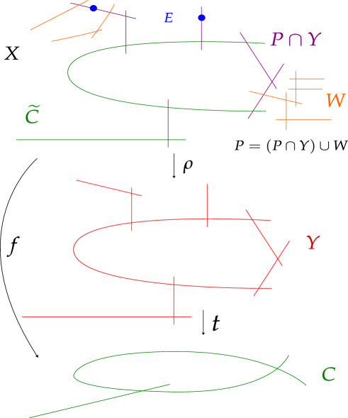
The following lemma was to make sense of B.2.4 above.
Lemma B.2.5.
Using notation for and as in B.2.4, we have . Moreover, is of the form , where and satisfy the following conditions:
-
(1)
is a partial normalization of at a finite set of its nodes,
-
(2)
is a genus semistable curve,
-
(3)
is contracted under the map , and
-
(4)
any connected component of is either contracted to a smooth point of , in which case it meets at a single smooth point, or the component is contracted to a node of , in which case it meets at both preimages of the node.
Proof.
We have that by the universal property of the coarse space . We now show satisfies the conditions as in the statement. Since has degree on each component of , it must be the union of a birational map with several contracted components, and hence must be of the form for a partial normalization of and the components which are contracted under the map. To conclude, we wish to show has properties and . First, since the genus of agrees with the genus of , each connected component of must have genus . Continuing to use that the genus of agrees with the genus of , if a connected component of is contracted to a node in , it must meet the two preimages of the node in nodally. Similarly, if a connected component is contracted to a smooth point, the only way has the same genus as is if that component of meets the preimage of that point in a single node, as claimed. ∎
Using the preceding notation, we are now ready to describe the relevant log structures on our twisted curves.
Notation B.2.6.
Using B.1.1, B.2.1, and B.2.2, let , denote the log stack whose underlying stack is with the log structure we describe next. For a scheme , suppose we have an point of , corresponding to a twisted stable map over . We endow with the log structure described in [Ols07, §3.10] obtained by viewing as an pointed twisted curve together with a degree divisor (so that, in particular, there is a copy of in over the marked gerbes and the degree marked gerbe on ). Similarly, has a canonical log structure from [Ols07, §3.10], and we endow with the pullback of this log structure along amalgamated with the log structure induced by the Cartier divisor (so in particular there is a copy of along the preimage of in ). We denote this log structure by .
In general may be different from when has more nodes than or has twisted nodes lying over the nodes of . If denotes the coarse space of with its log structure (including the points and degree divisor), and has log structure (including the degree divisor), then has the structure of a log map . We now describe the structure of this log map, see also [AMW14, Theorem B.6]. First, after replacing with an étale cover, so that factors as where is a composition of log blowups of and is a contraction of trees of rational curves lying over smooth unmarked points of . Using notation which restricts on geometric fibers to that in B.2.4 and Figure 7, is a sequence of log blowups of nodes and expansions of marked sections which contracts the chains of rational curves denoted and contracts the trees of rational curves denoted . Now is a morphism of log schemes by construction and is a morphism of log schemes since lies over the strict locus of and is an isomorphism away from . Thus the composition is a morphism of log schemes. Then, by composing the coarse space map with the above maps, we have a map of log stacks over .
Since the log structure on is pulled back from the log structure on , we obtain a corresponding commutative diagram
| (B.1) |
The points of , comprise all of the above data, with the log structure on for such an point given by .
The injective map of locally free log structures is not necessarily saturated due to the presence of twisted nodes in lying over nodes of . We let denote its saturation. Then is a simple extension (see, for example, [Ols07, Definition 1.5]) of locally free log structures.
B.3. Reducing to log smoothness
In this subsection we will show how log smoothness of the map implies our main result, Theorem B.1.1. We also deduce a generalization of Theorem B.1.1 where we allow the curve there to be nodal.
Proposition B.3.1.
With notation as in B.2.6, the log algebraic stack , is log smooth over .
We next record a version of Theorem B.1.1 for nodal curves. The reader may refer to B.2.1 and B.2.6 for notation used in the next statement. We say that a log smooth morphism is semistable if it is saturated and the source and target are regular with log structure given by a normal crossings divisors, see [IT14, Remark 3.6.6]. The reader may also wish to consult [AK00, Definition 0.1] and [ALT19, Subsection 4.2.1].
Theorem B.3.1.
is a normal crossings compactification of the locus of points corresponding to stable maps with smooth source and the log structure induced by the complementary divisor. Moreover, there is a factorization , where is semistable and is proper, quasifinite, log étale, and birational on each component of the source.
Remark B.3.2.
In the statement of Theorem B.3.1, is a union of components of the stack of simple extensions of log structures over as in [Ols07, Section 5.2] and it parameterizes certain twisted curves by the proof of [Ols07, Theorem 1.10].
Remark B.3.3.
We note that when , Theorem B.3.1 reduces to the well known statement that the forgetful map is semistable, where the moduli spaces of curves are equipped with their boundary log structures, parameterizing singular curves. The fiber over a geometric point representing a curve is a log smooth compactification of the configuration space of points on . This agrees with the Fulton-MacPherson compactification given in [FM94] when is smooth and .
B.3.2. Proof of Theorem B.1.1, Theorem B.3.1
We begin by explaining why Theorem B.1.1 and the first part of Theorem B.3.1 follow from B.3.1. Let denote either
-
(1)
the family from Theorem B.1.1 where is regular and has the trivial log structure or
-
(2)
the pullback of the universal family over along some strict map from a log scheme whose map of underlying stacks is étale.
We now verify that is log regular in the above two cases. Using [Ill02, 7.3(b)], the log scheme log regular in case . In case , note that with the trivial log structure is log regular by [Ill02, 7.3(b)]. Since is log smooth over , we obtain is also log smooth over . Hence is log regular by [Ill02, 7.3(c)].
We next show stable maps to such as above form a normal crossings compactification of the locus of such maps with smooth source. Using B.3.1, we find that is log smooth over . By [Ill02, 7.3(c)], is log regular. Note also that the log structure defined on coming from the divisor parameterizing singular covers is pulled back from that on , as follows from [Ols07, Theorem 1.10] and the proof of [Ols07, Lemma 5.1]. At a geometric point of , the characteristic monoid of the log structure described in [Ols07, §3.10] and the log structure on is described two lines before [Ols07, (3.6.6)]. This log structure is identified with , where is the number of nodes of the twisted curve corresponding to the point , so this log structure is locally free. Then, by [Ill02, 7.3(b)], we obtain that the log structure on is defined by a normal crossings divisor whose complement is the locus of triviality of the log structure and is regular. Since the open subset of triviality of the log structure on is precisely the locus of covers of curves with smooth source, we find that the above normal crossings divisor is that parameterizing the locus of covers where the source is singular. Finally, the fact that the locus of points in corresponding to stable maps with smooth source forms a dense open of follows from [Ill02, 7.3(d)]. This completes the proof of Theorem B.1.1 and the first part of Theorem B.3.1.
We conclude by now proving the second part of Theorem B.3.1. By the last paragraph of B.2.6, any -point of induces a simple extension where is the pullback of the log structure of along . Thus there is a map to a union of connected components of the stack of simple extensions of log structures ([Ols07, Section 5.2]) over , which we will denote by . Note that by representability of the map , the order of the simple extension is bounded by . Then is proper, quasi-finite, log étale, and birational on each component of the source by [Ols07, Lemma 5.3(ii)] and [Kat89, Proposition 3.4]. It follows that is a log smooth and saturated morphism where the source and target are regular with normal crossings log structures by the previous paragraph. This completes the proof. ∎
B.4. Verifying log smoothness
In the remainder of this section, we prove B.3.1, stating that is log smooth, which will also complete the proof of Theorem B.1.1.
We will approach B.3.1 via deformation theory. To begin understanding the deformation theory, we next describe the map on log cotangent sheaves associated to .
Remark B.4.1.
Given a geometric point of , using notation from B.2.4 and B.2.6, (where we use for what is called there,) there is an associated map . This induces a map which we now describe as a composition of three maps. First, recall that is a log curve over . Let denote the pullback of along . Then, the map factors through and the two versions of the relative logarithmic sheaf of differentials for these two log structures and are isomorphic. Hence, to describe we can endow with the log structure so that the map of log schemes is over the fixed base . First, there is a map , where is the log structure on from [Ols07, §3.10] obtained by forgetting the marked points and only remembering the degree divisor. Next, there is a map , for as in B.2.4 and the log structure on , including the degree divisor, but not including any of the marked points. And finally, we have a map . Note that . We can now identify the map as the composite map
| (B.2) |
where denotes the relative sheaf of logarithmic differentials associated to the log structure . Using [Kat00, Proposition 1.13], and the fact that the identification there is functorial for maps of log schemes, we can identify (B.2) with the sequence of maps
| (B.3) |
We denote the composite map in (B.3) by .
To better understand the deformation theory associated to a stable map, our first step will be to understand the map , whose pullback under is the first map in (B.3).
Lemma B.4.2.
For as in B.2.4, there is an isomorphism as well as an isomorphism .
Proof.
Write , for the union of components of not contained in , for as in B.2.4. For , we have an exact sequence
| (B.4) |
We can think of this sequence as expressing a local section of as a log differential on the normalization of with poles along and poles along the preimages of the nodes whose corresponding residues sum to zero. Observe that and . Hence, pushing forward (B.4) along , we get an exact sequence
| (B.5) |
Now, let . Note that is supported on , which is a disjoint union of points. By construction of , using B.2.5, each connected component of is a chain of ’s and consists of a degree two subscheme on each such connected component, with a degree point on each component on either end of the chain. Since the dualizing sheaf of has degree , this allows us to identify and hence is identified with . This is a skyscraper sheaf supported on , which we denote . Hence, the above sequence (B.5) becomes
| (B.6) |
We claim that this sequence expresses the condition that is the subsheaf of whose poles at preimages of a given node along the normalization map agree. Since also has this description, this will yield an identification . To verify our claim above, there are two cases. The easier case occurs in the neighborhood of a point of mapping to a smooth point of . Then, the map locally in a small neighborhood of such a point is identified with , and the kernel is , as claimed. The more difficult case is to compute the kernel at a nodal point of . Here, the fiber of is identified with a map given by . The first two copies of on the source correspond to the residues of the sheaf on the two preimages of the node in and the third copy of corresponds to the section on the contracted component of . Lying in the kernel of this map expresses the condition that the residues on each side of agree with the value on the contracted component of . Said another way, the values of the residues on each side of agree. This verifies our claim.
Finally, since we showed above the restriction of to any fiber of is the structure sheaf, the adjoint to our isomorphism restricts to an isomorphism on each contracted fiber of . Since also restricts to an isomorphism on , it is an isomorphism. ∎
We will see later that the log cotangent complex associated to a geometric point of as in B.2.4 can be identified with the two-term complex . The following lemma will therefore help us analyze the deformation theory of .
Proof.
We first describe the map , which was defined as a composition in B.4.1, in a more concrete fashion. Let denote the inclusion and the map contracting . The following statements can be obtained by unwinding the definitions of the maps induced on log differentials, used to define (B.3). The map in (B.3) is obtained as the pullback under of the isomorphism from B.4.2. The map in (B.3) is obtained from twisting the inclusion by . Finally, it remains to describe the map in (B.3). Since , There is an isomorphism which yields by adjunction a map . Define the map as that obtained via the inclusion . Then, and so the map is the composite of the maps
We now wish to identify the kernel of . First, the map is an isomorphism by B.4.2. The maps and are both injective maps of locally free sheaves by construction. Therefore, we can identify the kernel of with the kernel of . This map is an isomorphism away from , so we only need compute the kernel restricted to . On the map restricts to the map and so the kernel is indeed . Hence, the kernel of is , as claimed. ∎
We will see that the obstructions to deforming a point of as in B.2.4 lie in , for . Therefore, the next lemma will verify that deformations are unobstructed and hence be used to show is log smooth over .
Lemma B.4.4.
With notation as in B.2.4, let denote the two term complex on where the first term lies in degree and the second in degree . Then .
Proof.
First, we identify where , also in degrees . For the coarse space, and any line bundle on the adjunction map is an isomorphism, as can be verified locally using that is an isomorphism. Hence, because by [AB23, Proposition 3.11], we find . We also have
using that is étale, that by B.2.5, and that . The above observations yield the third isomorphism in the below chain of isomorphisms:
Therefore, it suffices to prove .
It follows from B.4.3 that sits in the following exact triangle
| (B.7) |
where the cokernel of the map . Applying to (B.7) and taking the long exact sequence yields the exact sequence
| (B.8) |
It is therefore enough to show that the first and third terms of (B.8) vanish. In general, by Serre duality, for a coherent sheaf on a Gorenstein curve , is dual to . From this, it follows that , as the st cohomology of any coherent sheaf vanishes.
To complete the proof, it remains only to show vanishes. Using Serre duality,
In the final step, we are using that each connected component of has arithmetic genus , since it is a union of irreducible components of the arithmetic genus curve , so . ∎
To prove B.3.1, we will discuss the deformation theory needed to deduce log smoothness of from the vanishing demonstrated in B.4.4. Note that parameterizes certain log structures on covers of curves, and we next introduce a stack parameterizing all fine log structures.
Notation B.4.5.
Using notation as in B.2.6 let denote the stack whose -points are tuples where is a fine log structure on , is a family of log twisted curves of type and is a log map such that is as in B.1.1. There is a map which sends an point of the source, thought of as a map with their log structures, as described in B.2.6, to the corresponding point of .
Combining the above lemmas with some deformation theory, we deduce B.3.1.
B.4.1. Proof of B.3.1
We note that is a proper algebraic stack by [AV02, Theorem 1.4.1], and hence is also a proper algebraic stack. To show is Deligne-Mumford, it suffices to show is Deligne-Mumford, which follows from [Ols07, Theorem 1.16].
To conclude the proof, we only need to verify that is log smooth over . Let denote a local Artin scheme over . Fix a point . Note that by B.2.6, has an induced log structure coming from pulling back the log structure from the associated map classifying , the coarse space of . Let denote a thickening of with . Suppose has residue field , maximal ideal , and assume . In order to verify formal smoothness, we wish to extend the above point to a point compatible with the above extension of log structure. First, we claim the obstruction to deforming our point above, viewed as a map of log stacks, lies in the hypercohomology group for in degrees . (We will soon show this is isomorphic to the complex as defined in B.4.4.) Indeed by [Ols05, Theorem 8.36(i)], there is a canonical obstruction in where is Gabber’s cotangent complex, as defined in [Ols05, Definition 8.5]. By [Ols05, Section 8.29] there is a transitivity triangle
and by [Ols05, Corollary 8.34 and Theorem 1.1(iii)], we can identify the map with ; here we use that log smooth curves are integral and that for a locally free sheaf. We next wish to show . There is an identification , where is the base change of along and is the base change of along , since is killed by . In order to show this vector space vanishes, we are free to base change to the algebraic closure of . Hence, for the remainder of the proof, we can assume is a geometric point as in B.2.4, and we aim to show .
To verify , we next claim we can identify and so that . By [Kat00, Proposition 1.13] we can identify . Then, by [AB23, Proposition 3.11], if denotes the coarse space map, . Arguing similarly, we also obtain . Therefore, the contangent complex is identified with . Now, note that , by B.4.4.
We are nearly done, and it only remains to explain why the vanishing of the obstruction space actually implies log smoothness of . To this end, let denote the algebraic stack classifying fine log schemes over , as defined in [Ols03, Section 5], and, in particular, [Ols03, Proposition 5.9]. Using B.4.5, the log structure on induces maps . The vanishing of implies the map above is formally smooth. The log structure from B.2.6 is the minimal log structure of the log map in the sense of [Wis16, p. 724] and so [Wis16, Theorem B.2] implies above is an open embedding. Therefore, the composite is formally smooth, hence smooth. It is shown in [Ols03, Theorem 4.6(ii) and (iii)] that if is a scheme with fine log structure then is log smooth if is smooth. From this, one can easily deduce the same holds in the case that is an algebraic stack with fine log structure by passing to a smooth cover of by a scheme. Hence, we obtain that is log smooth over , completing the proof. ∎
References
- [AB23] Kenneth Ascher and Dori Bejleri. Smoothability of relative stable maps to stacky curves. Épijournal Géom. Algébrique, 7:Art. 2, 22, 2023.
- [ACG11] Enrico Arbarello, Maurizio Cornalba, and Pillip A. Griffiths. Geometry of algebraic curves. Volume II, volume 268 of Grundlehren der Mathematischen Wissenschaften [Fundamental Principles of Mathematical Sciences]. Springer, Heidelberg, 2011. With a contribution by Joseph Daniel Harris.
- [ACGS20] Dan Abramovich, Qile Chen, Mark Gross, and Bernd Siebert. Punctured logarithmic maps. arXiv preprint arXiv:2009.07720v2, 2020.
- [Ach08] Jeffrey D. Achter. Results of Cohen-Lenstra type for quadratic function fields. In Computational arithmetic geometry, volume 463 of Contemp. Math., pages 1–7. Amer. Math. Soc., Providence, RI, 2008.
- [Ach23] Niven Achenjang. The average size of 2-selmer groups of elliptic curves in characteristic 2. arXiv preprint arXiv:2310.08493v2, 2023.
- [ACV03] Dan Abramovich, Alessio Corti, and Angelo Vistoli. Twisted bundles and admissible covers. volume 31, pages 3547–3618. 2003. Special issue in honor of Steven L. Kleiman.
- [AK00] D. Abramovich and K. Karu. Weak semistable reduction in characteristic 0. Invent. Math., 139(2):241–273, 2000.
- [ALT19] Karim Adiprasito, Gaku Liu, and Michael Temkin. Semistable reduction in characteristic 0, 2019.
- [AMW14] Dan Abramovich, Steffen Marcus, and Jonathan Wise. Comparison theorems for Gromov-Witten invariants of smooth pairs and of degenerations. Ann. Inst. Fourier (Grenoble), 64(4):1611–1667, 2014.
- [AV02] Dan Abramovich and Angelo Vistoli. Compactifying the space of stable maps. J. Amer. Math. Soc., 15(1):27–75, 2002.
- [BDPW23] Jonas Bergström, Adrian Diaconu, Dan Petersen, and Craig Westerland. Hyperelliptic curves, the scanning map, and moments of families of quadratic l-functions. arXiv preprint arXiv:2302.07664v2, 2023.
- [Bel04] Paolo Bellingeri. On presentations of surface braid groups. J. Algebra, 274(2):543–563, 2004.
- [Bis19] Matthew Bisatt. Explicit root numbers of abelian varieties. Trans. Amer. Math. Soc., 372(11):7889–7920, 2019.
- [BKL+15] Manjul Bhargava, Daniel M. Kane, Hendrik W. Lenstra, Jr., Bjorn Poonen, and Eric Rains. Modeling the distribution of ranks, Selmer groups, and Shafarevich-Tate groups of elliptic curves. Camb. J. Math., 3(3):275–321, 2015.
- [BKLOS19] Manjul Bhargava, Zev Klagsbrun, Robert J. Lemke Oliver, and Ari Shnidman. 3-isogeny Selmer groups and ranks of abelian varieties in quadratic twist families over a number field. Duke Math. J., 168(15):2951–2989, 2019.
- [BLR90] Siegfried Bosch, Werner Lütkebohmert, and Michel Raynaud. Néron models, volume 21 of Ergebnisse der Mathematik und ihrer Grenzgebiete (3) [Results in Mathematics and Related Areas (3)]. Springer-Verlag, Berlin, 1990.
- [BM23] Andrea Bianchi and Jeremy Miller. Polynomial stability of the homology of hurwitz spaces. arXiv preprint arXiv:2303.11194v1, 2023.
- [BS13a] Manjul Bhargava and Arul Shankar. The average number of elements in the 4-selmer groups of elliptic curves is 7. arXiv preprint arXiv:1312.7333v1, 2013.
- [BS13b] Manjul Bhargava and Arul Shankar. The average size of the 5-selmer group of elliptic curves is 6, and the average rank is less than 1. arXiv preprint arXiv:1312.7859v1, 2013.
- [BS15a] Manjul Bhargava and Arul Shankar. Binary quartic forms having bounded invariants, and the boundedness of the average rank of elliptic curves. Ann. of Math. (2), 181(1):191–242, 2015.
- [BS15b] Manjul Bhargava and Arul Shankar. Ternary cubic forms having bounded invariants, and the existence of a positive proportion of elliptic curves having rank 0. Ann. of Math. (2), 181(2):587–621, 2015.
- [BS23] Andrea Bianchi and Andreas Stavrou. Homology of configuration spaces of surfaces modulo an odd prime. arXiv preprint arXiv:2307.08664v1, 2023.
- [BSS21] Manjul Bhargava, Arul Shankar, and Ashvin Swaminathan. The second moment of the size of the -selmer group of elliptic curves. arXiv preprint arXiv:2110.09063v1, 2021.
- [BSW15] Manjul Bhargava, Arul Shankar, and Xiaoheng Wang. Geometry-of-numbers methods over global fields I: Prehomogeneous vector spaces. arXiv preprint arXiv:1512.03035v1, 2015.
- [Cad07] Charles Cadman. Using stacks to impose tangency conditions on curves. Amer. J. Math., 129(2):405–427, 2007.
- [Ces16] Kestutis Cesnavicius. Selmer groups as flat cohomology groups. J. Ramanujan Math. Soc., 31(1):31–61, 2016.
- [Cha97] Nick Chavdarov. The generic irreducibility of the numerator of the zeta function in a family of curves with large monodromy. Duke Math. J., 87(1):151–180, 1997.
- [Cha23] Kevin Chang. Hurwitz spaces, nichols algebras, and igusa zeta functions. arXiv preprint arXiv:2306.10446, 2023.
- [CLQR04] John Cremona, Joan-Carles Lario, Jordi Quer, and Kenneth Ribet, editors. Modular curves and abelian varieties, volume 224 of Progress in Mathematics. Birkhäuser Verlag, Basel, 2004. Papers from the conference held in Bellaterra, July 15–18, 2002.
- [Con14] Brian Conrad. Reductive group schemes. In Autour des schémas en groupes. Vol. I, volume 42/43 of Panor. Synthèses, pages 93–444. Soc. Math. France, Paris, 2014.
- [Det08] Michael Dettweiler. On the middle convolution of local systems. with an appendix by m. dettweiler and s. reiter. arXiv preprint arXiv:0810.3334v1, 2008.
- [dJ02] A. J. de Jong. Counting elliptic surfaces over finite fields. Mosc. Math. J., 2(2):281–311, 2002. Dedicated to Yuri I. Manin on the occasion of his 65th birthday.
- [DS23] Ariel Davis and Tomer M Schlank. The hilbert polynomial of quandles and colorings of random links. arXiv preprint arXiv:2304.08314v1, 2023.
- [ELS20] Jordan S. Ellenberg, Wanlin Li, and Mark Shusterman. Nonvanishing of hyperelliptic zeta functions over finite fields. Algebra Number Theory, 14(7):1895–1909, 2020.
- [ETW17] Jordan S Ellenberg, TriThang Tran, and Craig Westerland. Fox-neuwirth-fuks cells, quantum shuffle algebras, and malle’s conjecture for function fields. arXiv preprint arXiv:1701.04541v2, 2017.
- [EVW16] Jordan S. Ellenberg, Akshay Venkatesh, and Craig Westerland. Homological stability for Hurwitz spaces and the Cohen-Lenstra conjecture over function fields. Ann. of Math. (2), 183(3):729–786, 2016.
- [FGI+05] Barbara Fantechi, Lothar Göttsche, Luc Illusie, Steven L. Kleiman, Nitin Nitsure, and Angelo Vistoli. Fundamental algebraic geometry, volume 123 of Mathematical Surveys and Monographs. American Mathematical Society, Providence, RI, 2005. Grothendieck’s FGA explained.
- [FK88] Eberhard Freitag and Reinhardt Kiehl. Étale cohomology and the Weil conjecture, volume 13 of Ergebnisse der Mathematik und ihrer Grenzgebiete (3) [Results in Mathematics and Related Areas (3)]. Springer-Verlag, Berlin, 1988. Translated from the German by Betty S. Waterhouse and William C. Waterhouse, With an historical introduction by J. A. Dieudonné.
- [Fla90] Matthias Flach. A generalisation of the Cassels-Tate pairing. J. Reine Angew. Math., 412:113–127, 1990.
- [FLR23] Tony Feng, Aaron Landesman, and Eric M. Rains. The geometric distribution of Selmer groups of elliptic curves over function fields. Math. Ann., 387(1-2):615–687, 2023.
- [FM94] William Fulton and Robert MacPherson. A compactification of configuration spaces. Ann. of Math. (2), 139(1):183–225, 1994.
- [FS16] Jason Fulman and Dennis Stanton. On the distribution of the number of fixed vectors for the finite classical groups. Ann. Comb., 20(4):755–773, 2016.
- [Gol79] Dorian Goldfeld. Conjectures on elliptic curves over quadratic fields. In Number theory, Carbondale 1979 (Proc. Southern Illinois Conf., Southern Illinois Univ., Carbondale, Ill., 1979), volume 751 of Lecture Notes in Math, pages pp 108–118. Springer, Berlin, 1979.
- [Gre10] Aaron Greicius. Elliptic curves with surjective adelic Galois representations. Experiment. Math., 19(4):495–507, 2010.
- [Gro68] Alexander Grothendieck. Le groupe de Brauer. III. Exemples et compléments. In Dix exposés sur la cohomologie des schémas, volume 3 of Adv. Stud. Pure Math., pages 88–188. North-Holland, Amsterdam, 1968.
- [Gro23] Mark Gross. Remarks on gluing punctured logarithmic maps. arXiv preprint arXiv:2306.02661v1, 2023.
- [Hal08] Chris Hall. Big symplectic or orthogonal monodromy modulo . Duke Math. J., 141(1):179–203, 2008.
- [HB93] D. R. Heath-Brown. The size of Selmer groups for the congruent number problem. Invent. Math., 111(1):171–195, 1993.
- [HB94] D. R. Heath-Brown. The size of Selmer groups for the congruent number problem. II. Invent. Math., 118(2):331–370, 1994. With an appendix by P. Monsky.
- [HLHN14] Q. P. Hồ, V. B. Lê Hùng, and B. C. Ngô. Average size of 2-Selmer groups of elliptic curves over function fields. Math. Res. Lett., 21(6):1305–1339, 2014.
- [Hoa23] Anh Trong Nam Hoang. Fox-neuwirth cells, quantum shuffle algebras, and character sums of the resultant. arXiv preprint arXiv:2308.01410v1, 2023.
- [HS23] David Holmes and Pim Spelier. Logarithmic cohomological field theories. arXiv preprint arXiv:2308.01099v2, 2023.
- [HW10] Allen Hatcher and Nathalie Wahl. Stabilization for mapping class groups of 3-manifolds. Duke Math. J., 155(2):205–269, 2010.
- [Ill02] Luc Illusie. An overview of the work of K. Fujiwara, K. Kato, and C. Nakayama on logarithmic étale cohomology. Number 279, pages 271–322. 2002. Cohomologies -adiques et applications arithmétiques, II.
- [IT14] Luc Illusie and Michael Temkin. Exposé X. Gabber’s modification theorem (log smooth case). Number 363-364, pages 167–212. 2014. Travaux de Gabber sur l’uniformisation locale et la cohomologie étale des schémas quasi-excellents.
- [Kan13] Daniel Kane. On the ranks of the 2-Selmer groups of twists of a given elliptic curve. Algebra Number Theory, 7(5):1253–1279, 2013.
- [Kat89] K. Kato. Logarithmic structures of Fontaine-Illusie. In Algebraic analysis, geometry, and number theory (Baltimore, MD, 1988), pages 191–224. Johns Hopkins Univ. Press, Baltimore, MD, 1989.
- [Kat96] Nicholas M. Katz. Rigid local systems, volume 139 of Annals of Mathematics Studies. Princeton University Press, Princeton, NJ, 1996.
- [Kat00] Fumiharu Kato. Log smooth deformation and moduli of log smooth curves. Internat. J. Math., 11(2):215–232, 2000.
- [Kat02] Nicholas M. Katz. Twisted -functions and monodromy, volume 150 of Annals of Mathematics Studies. Princeton University Press, Princeton, NJ, 2002.
- [KMR13] Zev Klagsbrun, Barry Mazur, and Karl Rubin. Disparity in Selmer ranks of quadratic twists of elliptic curves. Ann. of Math. (2), 178(1):287–320, 2013.
- [Kow06] E. Kowalski. On the rank of quadratic twists of elliptic curves over function fields. Int. J. Number Theory, 2(2):267–288, 2006.
- [Lan21] Aaron Landesman. The geometric average size of Selmer groups over function fields. Algebra Number Theory, 15(3):673–709, 2021.
- [Lau81] G. Laumon. Semi-continuité du conducteur de Swan (d’après P. Deligne). In The Euler-Poincaré characteristic (French), volume 83 of Astérisque, pages 173–219. Soc. Math. France, Paris, 1981.
- [LPW09] David A. Levin, Yuval Peres, and Elizabeth L. Wilmer. Markov chains and mixing times. American Mathematical Society, Providence, RI, 2009. With a chapter by James G. Propp and David B. Wilson.
- [LST20] Michael Lipnowski, Will Sawin, and Jacob Tsimerman. Cohen-lenstra heuristics and bilinear pairings in the presence of roots of unity. arXiv preprint arXiv:2007.12533v1, 2020.
- [LT19] Michael Lipnowski and Jacob Tsimerman. Cohen-Lenstra heuristics for étale group schemes and symplectic pairings. Compos. Math., 155(4):758–775, 2019.
- [Mil80] James S. Milne. Étale cohomology, volume 33 of Princeton Mathematical Series. Princeton University Press, Princeton, N.J., 1980.
- [Moc95] Shinichi Mochizuki. The geometry of the compactification of the Hurwitz scheme. Publ. Res. Inst. Math. Sci., 31(3):355–441, 1995.
- [MPPRW24] Jeremy Miller, Peter Patzt, Dan Petersen, and Oscar Randal-Williams. Uniform twisted homological stability. arXiv preprint arXiv:2402.00354v1, 2024.
- [NW22] Hoi H Nguyen and Melanie Matchett Wood. Local and global universality of random matrix cokernels. arXiv preprint arXiv:2210.08526v1, 2022.
- [Ols03] Martin C. Olsson. Logarithmic geometry and algebraic stacks. Ann. Sci. École Norm. Sup. (4), 36(5):747–791, 2003.
- [Ols05] Martin C. Olsson. The logarithmic cotangent complex. Math. Ann., 333(4):859–931, 2005.
- [Ols07] Martin C. Olsson. (Log) twisted curves. Compos. Math., 143(2):476–494, 2007.
- [Par12] Brett Parker. Log geometry and exploded manifolds. Abh. Math. Semin. Univ. Hambg., 82(1):43–81, 2012.
- [PR12] Bjorn Poonen and Eric Rains. Random maximal isotropic subspaces and Selmer groups. J. Amer. Math. Soc., 25(1):245–269, 2012.
- [PW23] Sun Woo Park and Niudun Wang. On the Average of p-Selmer Ranks in Quadratic Twist Families of Elliptic Curves Over Global Function Fields. International Mathematics Research Notices, page rnad095, 05 2023.
- [Riz97] Ottavio Giulio Rizzo. On the variation of root numbers in families of elliptic curves. ProQuest LLC, Ann Arbor, MI, 1997. Thesis (Ph.D.)–Brown University.
- [Riz99] Ottavio G. Rizzo. Average root numbers in families of elliptic curves. Proc. Amer. Math. Soc., 127(6):1597–1603, 1999.
- [Riz03] Ottavio G. Rizzo. Average root numbers for a nonconstant family of elliptic curves. Compositio Math., 136(1):1–23, 2003.
- [RW20] Oscar Randal-Williams. Homology of Hurwitz spaces and the Cohen-Lenstra heuristic for function fields [after Ellenberg, Venkatesh, and Westerland]. Astérisque, (422):Exp. No. 1164, 469–497, 2020.
- [RWW17] Oscar Randal-Williams and Nathalie Wahl. Homological stability for automorphism groups. Adv. Math., 318:534–626, 2017.
- [Sab13] Maria Sabitova. Twisted root numbers and ranks of abelian varieties. J. Comb. Number Theory, 5(1):25–30, 2013.
- [Saw20] Will Sawin. Identifying measures on non-abelian groups and modules by their moments via reduction to a local problem. arXiv preprint arXiv:2006.04934v3, 2020.
- [SD08] Peter Swinnerton-Dyer. The effect of twisting on the 2-Selmer group. Math. Proc. Cambridge Philos. Soc., 145(3):513–526, 2008.
- [SGA72] Théorie des topos et cohomologie étale des schémas. Lecture Notes in Mathematics, Vol. 269. Springer-Verlag, Berlin, 1972. Séminaire de Géométrie Algébrique du Bois-Marie 1963–1964 (SGA 4), Dirigé par M. Artin, A. Grothendieck, et J. L. Verdier. Avec la collaboration de N. Bourbaki, P. Deligne et B. Saint-Donat.
- [Smi22] Alexander Smith. The distribution of -selmer groups in degree twist families i. arXiv preprint arXiv:2207.05674v2, 2022.
- [Sta] The Stacks Project Authors. Stacks Project. http://stacks.math.columbia.edu.
- [Sun12] Shenghao Sun. -series of Artin stacks over finite fields. Algebra Number Theory, 6(1):47–122, 2012.
- [SW23] Will Sawin and Melanie Matchett Wood. Conjectures for distributions of class groups of extensions of number fields containing roots of unity. arXiv preprint arXiv:2301.00791v1, 2023.
- [Tat63] John Tate. Duality theorems in Galois cohomology over number fields. In Proc. Internat. Congr. Mathematicians (Stockholm, 1962), pages 288–295. Inst. Mittag-Leffler, Djursholm, 1963.
- [Tay92] Donald E. Taylor. The geometry of the classical groups, volume 9 of Sigma Series in Pure Mathematics. Heldermann Verlag, Berlin, 1992.
- [Tho19] Jack A. Thorne. On the average number of 2-Selmer elements of elliptic curves over with two marked points. Doc. Math., 24:1179–1223, 2019.
- [TY14] Fabien Trihan and Seidai Yasuda. The -parity conjecture for abelian varieties over function fields of characteristic . Compos. Math., 150(4):507–522, 2014.
- [Vas03] A. Vasiu. Surjectivity criteria for -adic representations. I. Manuscripta Math., 112(3):325–355, 2003.
- [Ver67] J.-L Verdier. A duality theorem in the etale cohomology of schemes. In Proc. Conf. Local Fields (Driebergen, 1966), pages 184–198. Springer, Berlin, 1967.
- [Wew98] Stefan Wewers. Construction of Hurwitz spaces. Institut für Experimentelle Mathematik Essen, Ph.D. thesis, 1998.
- [Wew99] Stefan Wewers. Deformation of tame admissible covers of curves. In Aspects of Galois theory (Gainesville, FL, 1996), volume 256 of London Math. Soc. Lecture Note Ser., pages 239–282. Cambridge Univ. Press, Cambridge, 1999.
- [Wil09] Robert A. Wilson. The finite simple groups, volume 251 of Graduate Texts in Mathematics. Springer-Verlag London, Ltd., London, 2009.
- [Wis16] Jonathan Wise. Moduli of morphisms of logarithmic schemes. Algebra Number Theory, 10(4):695–735, 2016.
- [Woo17] Melanie Matchett Wood. The distribution of sandpile groups of random graphs. J. Amer. Math. Soc., 30(4):915–958, 2017.
- [Woo21] Melanie Matchett Wood. An algebraic lifting invariant of Ellenberg, Venkatesh, and Westerland. Res. Math. Sci., 8(2):Paper No. 21, 13, 2021.
- [Woo22] Melanie Matchett Wood. Probability theory for random groups arising in number theory. In Proc. Int. Cong. Math, volume 6, pages 4476–4508, 2022.
- [Zyw14] David Zywina. The inverse galois problem for orthogonal groups. arXiv preprint arXiv:1409.1151v1, 2014.