How Does GAN-based
Semi-supervised Learning Work?

First, we consider the optimal discriminator $D$ for any given generator $G$. Motivated by the proof of Proposition 1 in [4], this subsection proves that for fixed $G$, if the discriminator has infinite capacity, then regardless of whether the generator is perfect, i.e., $p_{G}=p$ or $p_{G}\neq p$, maximizing the above GAN-SSL objective $J_{D}$ is equivalent to maximizing the supervised learning objective $L_{D}$. We first introduce a basic Lemma 1 and give its proof.

Lemma 1 states that for any given generator and due to the infinite capacity of the discriminator, under the condition that the supervised objective remains unchanged, we can always increase the unsupervised objective until the extreme value is reached. Then, based on Lemma 1, we can present the theoretical results of the optimal discriminator $D$ for any given generator $G$.

Proposition 1 (1) and (2) jointly indicate that given a fixed generator, optimizing the discriminator of GAN-SSL is equivalent to optimizing that of supervised learning. Thus, the optimal discriminator in GAN-SSL is expected to be perfect on labeled data. We should note that Proposition $1$ of [4] gives a similar theoretical result, claiming only that the optimal discriminator of $L_{D}$ can lead to an optimal discriminator of GAN-SSL, i.e., the first claim of the above Proposition 1, but given the condition that $p_{G}=p$. Actually, our theoretical investigation instead shows that the condition $p_{G}=p$ is unnecessary and that the optimal discriminator of GAN-SSL is an optimal discriminator of supervised learning.

By carefully checking the statements in Proposition $1$ of [4] and comparing their results with ours, one may realize that their results are not rigorous. They claimed that good semi-supervised learning requires a bad generator because they observed that the semi-supervised objective shares the same generalization error with the supervised objective given a perfect generator. First, from our theoretical results, a perfect generator is not necessary for the observation, such that the requirement of a bad generator in their claim is unreasonable. Moreover, the fact that the semi-supervised objective shares the same generalization error with the supervised objective is insufficient for claiming that GAN-SSL will reduce the generalization ability of supervised learning. In addition, if we can claim only that the optimal discriminator of $L_{D}$ can lead to the optimal discriminator of GAN-SSL, one would not expect to obtain a perfect discriminator on labeled data by GAN-SSL such that the Assumption $1$ (1) of [4] is over-assumed. Our result, i.e., the Proposition 1 (2), can overcome their shortcoming, such that our later Assumption 1 (1) is indeed reasonable.

Next, for a fixed optimal discriminator, we discuss the behavior of the optimal generator of GAN-SSL. By the definition of the discriminator $D$, we have $P_{D}(K+1|x)={1}/{(1+\sum_{i=1}^{K}\exp(\omega_{i}^{T}f(x)))}$. Based on Proposition 1 (3), $P_{D}(K+1|x)={p_{G}(x)}/{(p(x)+p_{G}(x))}$. Namely,

implying that $\sum_{i=1}^{K}\exp(\omega_{i}^{T}f(x))=p(x)/p_{G}(x)$. Now, the objective of $G$ becomes $C(G)=L_{DG}+U_{G}$, with

The aim of the discriminator is to classify the labeled samples into the correct class, the unlabeled samples into the ”true” class (any of the first $K$ classes) and the generated samples into the ”fake” class, i.e., the $(K+1)$-th class. In this paper, the so-called perfect discriminator means that for any $(x,y)\in p(x,y)$, $P_{D}(y|x,y\leq K)>P_{D}(k|x,k\leq K,k\neq y)$, i.e., the discriminator can make a correct decision on labeled data. We say that the discriminator reaches its theoretical maximum given that $P_{D}(y|x,y\leq K)=1$ and, for any other class $k\neq y$, $P_{D}(k|x,k\leq K)=0$. Obviously, it is impossible to reach the theoretical maximum in practice, i.e., $P_{D}(y|x,y\leq K)$ can only be close to $1$, and for any other class $k\neq y$, $\exp(\omega_{k}^{T}f(x))\rightarrow 0$. That is, because the discriminator has an infinite capacity, we can expect that there exists $0<\epsilon\ll 1$ such that $(K-1)\exp(\omega_{k}^{T}f(x))\leq\epsilon$ for any other class $k\neq y$. Here, $\epsilon$ represents the error between the output of the perfect discriminator and its theoretical maximum. Now, we show the relationship between the true data distribution and the generator distribution in GAN-based semi-supervised tasks through the following Proposition 2.

Proposition 2 indicates that minimizing the generator objective $C(G)$ is equivalent to minimizing $JS(p||p_{G})$ and maximizing $KL(p||p-\epsilon p_{G})$ simultaneously. To minimize $JS(p||p_{G})$, we need to train $p_{G}$ close to $p$; however, to maximize $KL(p||p-\epsilon p_{G})$, we need to increase the difference between $p$ and $p-\epsilon p_{G}$. If the optimal solution $D$ of GAN-SSL for the supervised objective can reach the theoretical maximum, i.e., $\epsilon=0$, then minimizing $C(G)$ is equivalent to minimizing $JS(p||p_{G})$. Since the Jensen-Shannon divergence between two distributions is always non-negative and zero iff they are equal, then $C^{*}=-2\log 2$ is the global minimum of $C(G)$, and the only solution is $p_{G}=p$, i.e., the generator distribution perfectly replicates the true data distribution such that the optimal generator is perfect. Whereas, it is impossible to reach the theoretical maximum, then $\epsilon\neq 0$. If we assume that $\epsilon$ is sufficiently small, i.e., $0<\epsilon\ll 1$, the optimal generator $p_{G}$ will not be $p$. Otherwise, if $p_{G}=p$, $JS(p||p_{G})$ can reach its minimum, and $KL(p||p-\epsilon p_{G})=KL(p||p(1-\epsilon))$ becomes very small, which is in contrast to maximizing $KL(p||p-\epsilon p_{G})$ in the objective $C(G)$.

Different from the theoretical result of [4] that good semi-supervised learning requires a bad generator, Proposition 2 shows that the error of the optimal generator distribution relative to the true data distribution largely depends on the optimal discriminator. First, when the perfect discriminator for the supervised objective can reach its theoretical maximum, the global optimal generator of GAN-SSL is $p_{G}=p$, i.e., the optimal generator $G$ is perfect. However, since the theoretical maximum cannot be reached in practice, one cannot expect to learn a perfect generator, i.e., the optimal generator $G$ is imperfect. In addition, we note that although the optimal generator is imperfect in actual situations, it can be similar to the original data distribution. As shown in the work of [15], samples generated by the excellent GAN-SSL generator are not perfect but not completely different from the original data distribution, which is apparently inconsistent with the requirement of a ”bad” generator in [4].

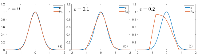
Case Study on Synthetic Data. To obtain a more intuitive understanding of Proposition 2, we conduct a case study based on a 1D synthetic dataset, where we can easily verify our theoretical analysis by visualizing the model behaviors. The training dataset is sampled from the Gaussian distribution $p=\mathcal{N}(0,0.4^{2})$. Based on Proposition 2, we study the relationship between the original data distribution $p$ and the generator distribution $p_{G}$ obtained by directly training the following generator objective function $C(G)=-KL(p||p-\epsilon p_{G})+2JS(p||p_{G})$. We use the generator architecture of a fully connected neural network with ReLU activations: 1-100-100-1. We give the results of comparing $p$ and $p_{G}$ when $\epsilon=0$, $\epsilon=0.1$ and $\epsilon=0.2$ in Figure 1, respectively. As theoretically analyzed above, for a constant $\epsilon=0$, minimizing $C(G)$ is equivalent to minimizing $JS(p||p_{G})$, and the optimal solution is $p_{G}=p$ (as shown in Figure 1 (a)). As shown in Figure 1 (b) and (c), when $\epsilon\neq 0$, $p_{G}$ is imperfect and the greater $\epsilon$ is, the larger the gap between $p_{G}$ and $p$. Although there is a certain gap between the generator distribution and the data distribution, $p_{G}$ is similar to $p$, and most of their supports overlap. Therefore, in this case, different from GANs, the optimal generator cannot be used to generate samples.

Finally, to study the behavior of the optimal discriminator of GAN-SSL on unlabeled data, we first present the assumption on the convergence conditions of the optimal discriminator and generator and the manifold conditions on the dataset. Let $\Omega_{\mathcal{L}}$ be the set of labeled data. Let $\Omega$, $\Omega_{\mathcal{G}}$ be the data manifold and generated data manifold, respectively. Obviously, we have $\Omega_{\mathcal{L}}\subset\Omega$, and the unlabeled data should be sampled from $\Omega\setminus\Omega_{\mathcal{L}}$. Denote $\Omega=\cup_{k=1}^{K}\Omega^{k}$, where $\Omega^{k}$ is the data manifold of class $k$. Denote $\Omega^{k}=\cup_{l}\Omega^{kl}$, where $\Omega^{kl}$ is a connected subdomain.

The Reasonableness of Assumption 1 (1). According to the theoretical analysis for the optimal discriminator (Proposition 1), we found that optimizing the discriminator of GAN-SSL is equivalent to optimizing that of supervised learning. Because $D$ is an optimal solution of the GAN-SSL objective, $D$ is an optimal solution of the supervised learning objective. Naturally, Assumption 1 (1) holds, i.e., the discriminator has a correct decision boundary for labeled data given that the discriminator has infinite capacity.

The Reasonableness of Assumption 1 (2). Proposition 2 implies that the optimal generator we obtain in practice is not a perfect generator such that we assume $\Omega_{\mathcal{G}}\setminus\bar{\Omega}\neq\emptyset$. We ignore the case of $\Omega_{\mathcal{G}}\subset\Omega,\Omega\setminus\bar{\Omega}_{\mathcal{G}}\neq\emptyset$ since it is almost impossible to ensure that our optimal generator can output only true data but with different probabilities in practice, unless we obtain the worst model with model collapse. Similar to [4], we also make a strong assumption regarding the true-fake correctness of the true data ($\Omega$) and fake data ($\Omega_{\mathcal{G}}\setminus\bar{\Omega}$). In other words, we assume that the sampling of unlabeled data is good enough to achieve the best generalization ability on the true data manifold.

The Reasonableness of Assumption 1 (3). Intuitively, one cannot expect to achieve a good classification performance on a connected subdomain with no label information, since we can optionally set this connected subdomain to any class but with no influence on the objective.

The Reasonableness of Assumption 1 (4). Apparently, Assumption 1 (3) is a sufficient condition for this assumption. In addition, since the optimal generator is imperfect and we need only its existence, one can expect to be able to achieve this condition.

Now, based on Assumption 1, we give the main result of this subsection.

We remark that the proof of Proposition 3 is similar to that in [4] but with different conditions; see the supplementary material for more details. Proposition 3 guarantees that given the convergence conditions of the optimal discriminator and generator, which are induced by Proposition 1 and 2, respectively, if the labeled data can traverse all subdomains of the data manifold, then the discriminator $D$ will be perfect on the data manifold, i.e., it can also learn correct decision boundaries for all unlabeled data. Now, we discuss the difference between our Assumption 1 and Assumption $1$ in [4].

1. 1.

   As discussed above in subsection $3.1$, the first Assumption $1$ (1) in [4] is over-assumed, since they cannot expect to obtain a perfect discriminator by optimizing the GAN-SSL objective. However, our Proposition 1 can support our Assumption 1 (1).

2. 2.

   Their Assumption $1$ (2) and Assumption $1$ (3) correspond to our Assumption 1 (2). We all assume that the optimal $D$ can result in a perfect decision regarding true-fake correctness. However, since our optimal $G$ is not a bad one, as a result of Proposition 2, we assume only that the data in $\Omega_{\mathcal{G}}\setminus\bar{\Omega}$ are fake.

3. 3.

   Unlike [4], we additionally give a reasonable assumption on the data manifold, i.e, Assumption 1 (3). By a careful check, one can find that the authors of [4] ignore this assumption because they implicitly assume that after embedding $f$, the feature space of each class is a connected domain. Otherwise, the proof of their Proposition $2$ is not correct, since one can set a connected subdomain of the feature space $F_{k}$ without label information to any class by a similar contradiction proof.

4. 4.

   Similar to our Assumption 1 (4), [4] make a stronger assumption before the definition of their Assumption $1$ by setting $G$ as a complement generator. Given a complement generator, our Assumption 1 (4) can clearly be satisfied. Note that under their definition, if the optimal generator $G$ is a complementary one, the feature space of the generated data will fill the complement set of the feature space of the true data. In other words, they hope that the ”bad” generator can not only generate fake data but also generate all the existing fake data. Apparently, this assumption is too strong and requires the generator to offer a high representation ability, since our true data manifold is always low-dimensional. However, we need only the existence of a generated fake data point such that its feature can be linearly represented by that of two true data points with at least one labeled data point. This existence has a high probability to be satisfied given only a connected subdomain $\Omega^{jl}$ and an imperfect generator. Here, we actually release the requirement for a complement generator.

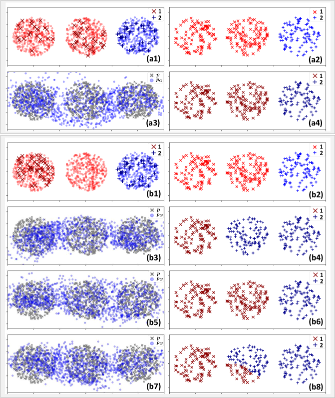
The Reasonableness of Assumption 1 (3) on Synthetic Data. We design a binary classification problem with $\Omega=\Omega^{1}\cup\Omega^{2}$, where $\Omega^{1}=\Omega^{11}\cup\Omega^{12}$ and $\Omega^{11}$, $\Omega^{12}$ and $\Omega^{2}$ are three bounded 2D circles with no interaction. The unlabeled data are uniformly sampled from $\Omega$. If Assumption 1 (3) is satisfied, each connected domain contains at least one labeled data point, as shown in Figure 2 (a1). Then, as shown in Figure 2 (a4), we can easily train the discriminator to learn the correct decision boundary. However, if Assumption 1 (3) is not satisfied, for the data in class $1$, we sample only the labeled data in subdomain $\Omega^{11}$, as shown in Figure 2 (b1). At this time, it is difficult for the discriminator to learn a correct decision boundary. As shown in Figure 2 (b4), (b6), and (b8), we choose three kinds of results under several training processes. For the unlabeled data in subdomain $\Omega^{12}$, the classification results are uncertain. Hence, a comparison between Figure 2 (a4), (b4), (b6), and (b8) can show that the condition of Assumption 1 (3) is necessary to obtain a perfect discriminator on unlabeled data. Furthermore, as shown in Figure 2 (a3), (b3), (b5) and (b7), a comparison of the generated samples shows that there is indeed a certain gap between the generator distribution and the data distribution, while the optimal generator is not a complementary one, as claimed in [4].

References

- [1] Sanjeev Arora, Rong Ge, Yingyu Liang, Tengyu Ma, and Yi Zhang. Generalization and equilibrium in generative adversarial nets (GANs). In International Conference on Machine Learning, pages 224–232, 2017.
- [2] Yu Bai, Tengyu Ma, and Andrej Risteski. Approximability of discriminators implies diversity in GANs. In International Conference on Learning Representations, 2019.
- [3] David Berthelot, Nicholas Carlini, Ian Goodfellow, Nicolas Papernot, Avital Oliver, and Colin A Raffel. MixMatch: A holistic approach to semi-supervised learning. In Neural Information Processing Systems, pages 5049–5059, 2019.
- [4] Zihang Dai, Zhilin Yang, Fan Yang, William W. Cohen, and Ruslan Salakhutdinov. Good semi-supervised learning that requires a bad GAN. In Neural Information Processing Systems, 2017.
- [5] Jinhao Dong and Tong Lin. MarginGAN: Adversarial training in semi-supervised learning. In Neural Information Processing Systems, pages 10440–10449, 2019.
- [6] Zhe Gan, Liqun Chen, Weiyao Wang, Yuchen Pu, Yizhe Zhang, Hao Liu, Chunyuan Li, and Lawrence Carin. Triangle generative adversarial networks. In Neural Information Processing Systems, pages 5247–5256, 2017.
- [7] Ian Goodfellow, Jean Pouget-Abadie, Mehdi Mirza, Bing Xu, David Warde-Farley, Sherjil Ozair, Aaron Courville, and Yoshua Bengio. Generative adversarial nets. In Neural Information Processing Systems, pages 2672–2680, 2014.
- [8] Diederik P. Kingma, Danilo J. Rezende, Shakir Mohamed, and Max Welling. Semi-supervised learning with deep generative models. In Neural Information Processing Systems, pages 3581–3589, 2014.
- [9] Diederik P Kingma and Max Welling. Auto-encoding variational bayes. In International Conference on Learning Representations, 2014.
- [10] Thomas N. Kipf and Max Welling. Semi-supervised classification with graph convolutional networks. In International Conference on Learning Representations, 2017.
- [11] Samuli Laine and Timo Aila. Temporal ensembling for semi-supervised learning. In International Conference on Learning Representations, 2017.
- [12] Bruno Lecouat, Chuan Sheng Foo, Houssam Zenati, and Vijay Chandrasekhar. Manifold regularization with GANs for semi-supervised learning. arXiv preprint arXiv:1807.04307, 2018.
- [13] Chongxuan Li, Taufik Xu, Jun Zhu, and Bo Zhang. Triple generative adversarial nets. In Neural Information Processing Systems, pages 4088–4098, 2017.
- [14] Lars Mescheder, Andreas Geiger, and Sebastian Nowozin. Which training methods for GANs do actually converge? International Conference on Machine Learning, 2018.
- [15] Tim Salimans, Ian Goodfellow, Wojciech Zaremba, Vicki Cheung, Alec Radford, and Chen Xi. Improved techniques for training GANs. In Neural Information Processing Systems, 2016.
- [16] Tim Salimans, Han Zhang, Alec Radford, and Dimitris Metaxas. Improving GANs using optimal transport. In International Conference on Learning Representations, 2018.
- [17] Jost Tobias Springenberg. Unsupervised and semi-supervised learning with categorical generative adversarial networks. In International Conference on Learning Representations, 2016.
- [18] Aäron van den Oord, Sander Dieleman, Heiga Zen, Karen Simonyan, Oriol Vinyals, Alexander Graves, Nal Kalchbrenner, Andrew Senior, and Koray Kavukcuoglu. Wavenet: A generative model for raw audio. SSW, page 125, 2016.
- [19] Qizhe Xie, Zihang Dai, Eduard Hovy, Minh-Thang Luong, and Quoc V. Le. Unsupervised data augmentation for consistency training. arXiv preprint arXiv:1904.12848, 2019.
Appendix
Proof of Proposition
Proof.
Proof of Proposition (1). Similar to the proof of Lemma , given an optimal solution of the supervised objective , due to the discriminator has infinite capacity, there exists such that for all and ,