How many classifiers do we need?
Abstract
As performance gains through scaling data and/or model size experience diminishing returns, it is becoming increasingly popular to turn to ensembling, where the predictions of multiple models are combined to improve accuracy. In this paper, we provide a detailed analysis of how the disagreement and the polarization (a notion we introduce and define in this paper) among classifiers relate to the performance gain achieved by aggregating individual classifiers, for majority vote strategies in classification tasks. We address these questions in the following ways. (1) An upper bound for polarization is derived, and we propose what we call a neural polarization law: most interpolating neural network models are 4/3-polarized. Our empirical results not only support this conjecture but also show that polarization is nearly constant for a dataset, regardless of hyperparameters or architectures of classifiers. (2) The error of the majority vote classifier is considered under restricted entropy conditions, and we present a tight upper bound that indicates that the disagreement is linearly correlated with the target, and that the slope is linear in the polarization. (3) We prove results for the asymptotic behavior of the disagreement in terms of the number of classifiers, which we show can help in predicting the performance for a larger number of classifiers from that of a smaller number. Our theories and claims are supported by empirical results on several image classification tasks with various types of neural networks.
1 Introduction
As performance gains through scaling data and/or model size experience diminishing returns, it is becoming increasingly popular to turn to ensembling, where the predictions of multiple models are combined, both to improve accuracy and to form more robust conclusions than any individual model alone can provide. In some cases, ensembling can produce substantial benefits, particularly when increasing model size becomes prohibitive. In particular, for large neural network models, deep ensembles LPB (17) are especially popular. These ensembles consist of independently trained models on the same dataset, often using the same hyperparameters, but starting from different initializations.
The cost of producing new classifiers can be steep, and it is often unclear whether the additional performance gains are worth the cost. Assuming that constructing two or three classifiers is relatively cheap, procedures capable of deciding whether to continue producing more classifiers are needed. To do so requires a precise understanding of how to predict ensemble performance. Of particular interest are majority vote strategies in classification tasks, noting that regression tasks can also be formulated in this way by clustering outputs. In this case, one of the most effective avenues for predicting performance is the disagreement JNBK (22); BJRK (22): measuring the degree to which classifiers provide different conclusions over a given dataset. Disagreement is concrete, easy to compute, and strongly linearly correlated with majority vote prediction accuracy, leading to its use in many applications. However, a priori, the precise linear relationship between disagreement and accuracy is unclear, preventing the use of disagreement for predicting ensemble performance.
Our goal in this paper is to go beyond disagreement-based analysis to provide a more quantitative understanding of the number of classifiers one should use to achieve a desired level of performance in modern practical applications, in particular for neural network models. In more detail, our contributions are as follows.
-
(i)
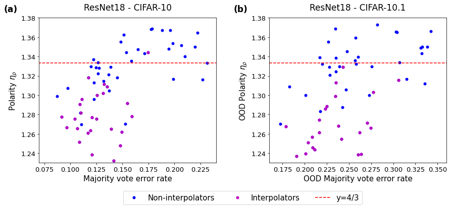
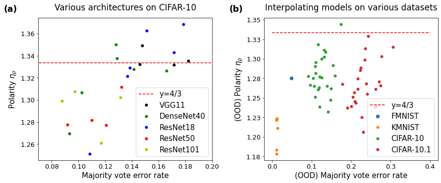
We introduce and define the concept of polarization, a notion that measures the higher-order dispersity of the error rates at each data point, and which indicates how polarized the ensemble is from the ground truth. We state and prove an upper bound for polarization (Theorem 1). Inspired by the theorem, we propose what we call a neural polarization law (Conjecture 1): most interpolating (Definition 2) neural network models are 4/3-polarized. We provide empirical results supporting the conjecture (Figures 1 and 2).
-
(ii)
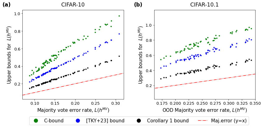
Using the notion of polarization, we develop a refined set of bounds on the majority vote test error rate. For one, we provide a sharpened bound for any ensembles with a finite number of classifiers (Corollary 1). For the other, we offer a tighter-than-ever bound under an additional condition on the entropy of the ensemble (Theorem 4). We provide empirical results that demonstrate our new bounds perform significantly better than the existing bounds on the majority vote test error (Figure 3).
-
(iii)
The asymptotic behavior of the majority vote error rate is determined as the number of classifiers increases (Theorem 5). Consequently, we show that we can predict the performance for a larger number of classifiers from that of a smaller number. We provide empirical results that show such predictions are considerably accurate across various pairs of model architecture and dataset (Figure 4).
In Section 2, we define the notations that will be used throughout the paper, and we introduce upper bounds for the error rate of the majority vote from previous work. The next three sections are the main part of the paper. In Section 3, we introduce the notion of polarization, , which plays a fundamental role in relating the majority vote error rate to average error rate and disagreement. We explore the properties of the polarization and present empirical results that corroborate our claims. In Section 4, we present tight upper bounds for the error rate of the majority vote for ensembles that satisfy certain conditions; and in Section 5, we prove how disagreement behaves in terms of the number of classifiers. All of these ingredients are put together to estimate the error rate of the majority vote for a large number of classifiers using information from only three sampled classifiers. In Section 6, we provide a brief discussion and conclusion. Additional material is presented in the appendices.
2 Preliminaries
In this section, we introduce notation that we use throughout the paper, and we summarise previous work on the performance of the majority vote error rate.
2.1 Notations
We focus on -class classification problems, with features , labels and feature-label pairs . A classifier is a function that maps a feature to a label. We define the error rate of a single classifier , and the disagreement and the tandem loss MLIS (20) between two classifiers, and , as the following:
| Error rate : | |||
| Disagreement : | |||
| Tandem loss : |
where the expectation is used to denote . Next, we consider a distribution of classifiers, , which may be viewed as an ensemble of classifiers. This distribution can represent a variety of different cases. Examples include: (1) a discrete distribution over finite number of , e.g., a weighted sum of ; and (2) a distribution over a parametric family , e.g., a distribution of classifiers resulting from one or multiple trained neural networks. Given the ensemble , the (weighted) majority vote is defined as
Again, denotes , and we use for , respectively, throughout the paper. In this sense, represents the average error rate under a distribution of classifiers and represents the average disagreement between classifiers under . Hereafter, we refer to , , and as the average error rate, the disagreement, and the majority vote error rate, respectively, with
Lastly, we define the point-wise error rate, , which will serve a very important role in this paper (for clarity, we will denote by unless otherwise necessary):
| (1) |
2.2 Bounds on the majority vote error rate
The simplest relationship between the majority vote error and the average error rate was introduced in McA (98). It states that the error in the majority vote classifier cannot exceed twice the average error rate:
| (2) |
A simple proof for this relationship can be found in MLIS (20) using Markov’s inequality. Although (2) does not provide useful information in practice, it is worth noting that this bound is, in fact, tight. There exist pathological examples where exhibits twice the average error rate (see Appendix C in TKY+ (24)). This suggests that we can hardly obtain a useful or tighter bound by relying on only the “first-order” term, .
Accordingly, more recent work constructed bounds in terms of “second-order” quantities, and . In particular, LMRR (17) and MLIS (20) designed a so-called C-bound using the Chebyshev-Cantelli inequality, establishing that, if , then
| (3) |
As an alternative approach, MLIS (20) incorporated the disagreement into the bound as well, albeit restricted to the binary classification problem, to obtain:
| (4) |
While (3) and (4) may be tighter in some cases, once again, there do exist pathological examples where this bound is as uninformative as the first-order bound (2). Motivated by these weak results, TKY+ (24) take a new approach by restricting to be a “good ensemble,” and introducing the competence condition (see Definition 3 in our Appendix A). Informally, competent ensembles are those where it is more likely—in average across the data—that more classifiers are correct than not. Based on this notion, TKY+ (24) prove that competent ensembles are guaranteed to have weighted majority vote error smaller than the weighted average error of individual classifiers:
| (5) |
That is, the majority vote classifier is always beneficial. Moreover, TKY+ (24) proves that any competent ensemble of -class classifiers satisfy the following inequality.
| (6) |
We defer further discussion of competence to Appendix A, where we introduce simple cases for which competence does not hold. In these cases, we show how one can overcome this issue so that the bounds (5) and (6) still hold. In particular, in Appendix A.3, we provide an example to show the bound (6) is tight.
3 The Polarization of an Ensemble
In this section, we introduce a new quantity, , which we refer to as the polarization of an ensemble . First, we provide examples as to what this quantity represents and draw a connection to previous studies. Then, we present theoretical and empirical results that show this quantity plays a fundamental role in relating the majority vote error rate to average error rate and disagreement. In Theorem 1, we prove an upper bound for the polarization , which highlights a fundamental relationship between the polarization and the constant . Inspired from the theorem, we propose Conjecture 1 which we call a neural polarization law. Figures 1 and 2 present empirical results on an image recognition task that corroborates the conjecture.
We start by defining the polarization of an ensemble. In essence, the polarization is an improved (smaller) coefficient on the Markov’s inequality on , where is the point-wise error rate defined as equation (1). It measures how much the ensemble is “polarized” from the truth, with consideration of the distribution of .
Definition 1 (Polarization).
An ensemble is -polarized if
| (7) |
The polarization of an ensemble is
| (8) |
which is the smallest value of satisfies inequality (7).
Note that the polarization always takes a value in , due to the positivity constraint and Markov’s inequality. Also note that ensemble with polarization is -polarized for any .
To understand better what this quantity represents, consider the following examples. The first example demonstrates that polarization increases as the majority vote becomes more polarized from the truth, while the second example demonstrates how polarization increases when the constituent classifiers are more evenly split.
Example 1.
Consider an ensemble where 75% of classifiers output Label 1 with probability one, and the other 25% classifiers output Label 2 with probability one.
-
-
Case 1. The true label is Label 1 for the whole data.
In this case, the majority vote in results in zero error rate. The point-wise error rate is on the entire dataset, and thus . The polarization is . -
-
Case 2. The true label is Label 1 for half of the data and is Label 2 for the other half.
In this case, the majority vote is only correct for half of the data. The point-wise error rate is for this half, and is for the other half. The polarization is . -
-
Case 3. The true label is Label 2 for the whole data.
In this case, the majority vote in is wrong on every data point. The point-wise error rate is on the entire dataset and thus . The polarization is .
Example 2.
Now consider an ensemble of which 51% of classifiers always output Label 1, and the other 49% classifiers always output Label 2.
-
-
Case 1. The polarization is now , the same as in Example 1.
-
-
Case 2. The polarization is , which is larger than in Example 1.
-
-
Case 3. The polarization is now , which is larger than in Example 1.
In addition, the following proposition draws a connection between polarization and the competence condition mentioned in Section 2.2. It states that the polarization of competent ensembles cannot be very large. The proof is deferred to Appendix A.2.
Proposition 1.
Competent ensembles are -polarized.
Now we delve more into this new quantity. We introduce Theorem 1, which establishes (by means of concentration inequalities) an upper bound on the polarization . The proof of Theorem 1 is deferred to Appendix B.1.
Theorem 1.
Let be independent and identically distributed samples from that are independent of an ensemble . Then the polarization of the ensemble, , satisfies
| (9) |
with probability at least , where and .
Surprisingly, in practice, appears to be a good choice for a wide variety of cases. See Figure 1 and Figure 2, which show the polarization obtained from VGG11 SZ (14), DenseNet40 HLVDMW (17), ResNet18, ResNet50 and ResNet101 HZRS (16) trained on CIFAR-10 Kri (09) with various hyperparameters choices. The trend does not deviate even when evaluated on an out-of-distribution dataset, CIFAR-10.1 RRSS (18); TFF (08). For more details on these empirical results, see Appendix C.
Remark.
We emphasize that values for that are larger than does not contradict Theorem 1. This happens when the non-constant second term in (9) is larger than , which is often the case for classifiers which are not interpolating (or, indeed, that underfit or perform poorly).
Definition 2 (Interpolating, BHMM (19)).
A classifier is interpolating if it achieves an accuracy of 100% on the training data.
Putting Theorem 1 and the consistent empirical trend shown in Figure 2(b) together, we propose the following conjecture.
Conjecture 1 (Neural Polarization Law).
The polarization of ensembles comprised of independently trained interpolating neural networks is smaller than .
4 Entropy-Restricted Ensembles
In this section, we first present an upper bound on the majority vote error rate, , in Theorem 2, using our notion of polarization which we introduced and defined in the previous section. Then, we present Theorems 3 and 4 which are the main elements in obtaining tighter upper bounds on . Figure 3 shows our proposed bound offers a significant improvement over state-of-the-art results. The new upper bounds are inspired from the fact that classifier prediction probabilities tend to concentrate on a small number of labels, rather than be uniformly spread over all the possible labels. This is analogous to the phenomenon of neural collapse Kot (22). As an example, in the context of a computer vision model, when presented with a photo of a dog, one might expect that a large portion of reasonable models might classify the photo as an animal other than a dog, but not as a car or an airplane.
We start by stating an upper bound on the majority vote error, as a function of polarization . This upper bound is tighter (smaller) than the previous bound in inequality (6) when the polarization is lower than , which is the case for competent ensembles. The proof is deferred to Appendix B.2.
Theorem 2.
For an ensemble of -class classifiers,
where is the polarization of the ensemble .
Based on the upper bound stated in Theorem 2, we add a restriction on the entropy of constituent classifiers to obtain Theorem 3. The theorem provides a tighter scalable bound that does not have explicit dependency on the total number of labels, with a small cost in terms of the entropy of constituent classifiers. The proof of Theorem 3 is deferred to Appendix B.3.
Theorem 3.
Let be any -polarized ensemble of -class classifiers that satisfies , where and , for all data points . Then, we have
While Theorem 3 might provide a tighter bound than prior work, coming up with pairs that satisfy the constraint is not an easy task. This is not an issue for a discrete ensemble, however. If is a discrete distribution of classifiers, then we observe that the assumption of Theorem 3 must always hold with . We state this as the following corollary.
Corollary 1 (Finite Ensemble).
For an ensemble that is a weighted sum of classifiers, we have
| (10) |
where is the polarization of the ensemble .
.
See Figure 3, which provides empirical results that compare the bound in Corollary 1 with the C-bound in inequality (3), and with inequality (6) proposed in TKY+ (24). We can observe that the new bound in Corollary 1 is strictly tighter than the others. For more details on these empirical results, see Appendix C.
Although the bound in Corollary 1 is tighter than the bounds from previous studies, it’s still not tight enough to use it as an estimator for . In the following theorem, we use a stronger condition on the entropy of an ensemble to obtain a tighter bound. The proof is deferred to Appendix B.4.
Theorem 4.
For any -polarized ensemble that satisfies
| (11) |
we have
The condition (11) can be rephrased as follows: compared to the error , the entropy of the distribution of wrong predictions is small, and it is concentrated on a small number of labels. A potential problem is that one must know or estimate the smallest possible value of in advance. At least, we can prove that always satisfies the condition (11) for an ensemble of -class classifiers. The proof is deferred to Appendix B.4.
Corollary 2.
For any -polarized ensemble of K-class classifiers, we have
Naturally, this is not good enough for our goal. We discuss more on how to estimate the smallest possible value of in the following section.
5 A Universal Law for Ensembling
In this section, our goal is to predict the majority vote error rate of an ensemble with large number of classifiers by just using information we can obtain from an ensemble with a small number, e.g., three, of classifiers. Among the elements in the bound in Theorem 4,
we plug in as a result of Theorem 1; and since is invariant to the number of classifiers, it remains to predict the behavior of and the smallest possible value of , . Since the denominator is invariant to the number of classifiers, and the numerator resembles the disagreement between classifiers, is expected to follow a similar pattern as . Note that the numerator of has the same form as the disagreement, differing by only one less label. Both are -statistics that can be expressed as a multiple of a -statistic, as shown in equation (5). In the next theorem, we show that the disagreement for a finite number of classifiers can be expressed as the sum of a hyperbolic curve and an unbiased random walk. Here, denotes the greatest integer less than or equal to and is the Skorokhod space on (see Appendix B.5).
Theorem 5.
Let denote an empirical distribution of independent classifiers sampled from a distribution and . Then, there exists such that
where , and converges weakly to a standard Wiener process in as .
Proof.
Let . We observe that
| (12) |
which is a -statistic with the kernel function . Let .
The invariance principle of -statistics (Theorem 7 in Appendix B.5) states that the process , defined by and , converges weakly to a standard Wiener process in as , since . Therefore, converges in probability as to .
Letting , we can express as , with and . Since , it follows by Slutsky’s Theorem that converges weakly to a standard Wiener process in as . ∎
Theorem 5 suggests that the disagreement within classifiers, , can be approximated as . From the disagreement within classifiers, can be approximated as , and therefore we get
| (13) |
Assume that we have three classifiers sampled from . We denote the average error rate, the disagreement, and the from these three classifiers by , , and , respectively. Then, from Theorem 4 and approximation (13) (which applies to both disagreement and ), we estimate the majority vote error rate of classifiers from as the following:
| (14) |
Alternatively, we can use the polarization measured from three classifiers, , instead of , to obtain:
| (15) |
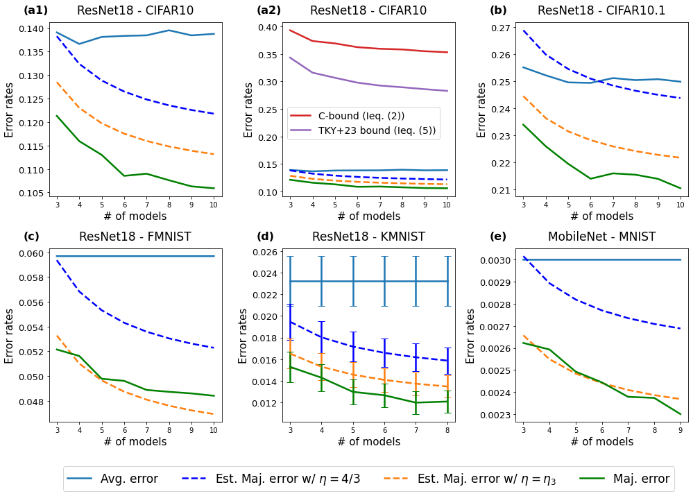
Figure 4 presents empirical results that compare the estimated (extrapolated) majority vote error rates in equations (5) and (15) with the true majority vote error for each number of classifiers. ResNet18 models are tested on four different dataset: CIFAR-10, CIFAR-10.1, Fashion-MNIST XRV (17) and Kuzushiji-MNIST CBIK+ (18) where the models are trained on the corresponding train data. MobileNet How (17) is trained and tested on the MNIST Den (12) dataset. Not only do the estimators show significant improvement compared to the bounds introduced in Section 2.2, we observe that the estimators are very close to the actual majority vote error rate; and thus the estimators have practical usages, unlike the bounds from previous studies. In Figure 4(a2), existing bounds (3) and (6) are much larger compared to the average error rate. This is also the case for (architecture, dataset) pairs of other subplots.
6 Discussion and Conclusion
This work addresses the question: how does the majority vote error rate change according to the number of classifiers? While this is an age-old question, it is one that has received renewed interest in recent years. On the journey to answering the question, we introduce several new ideas of independent interest. (1) We introduced the polarization , of an ensemble of classifiers. This notion plays an important role throughout this paper and appears in every upper bound presented. Although Theorem 1 gives some insight into polarization, our conjectured neural polarization law (Conjecture 1) is yet to be proved or disproved, and it provides an exciting avenue for future work. (2) We proposed two classes of ensembles whose entropy is restricted in different ways. Without these constraints, there will always be examples that saturate even the least useful majority vote error bounds. We believe that accurately describing how models behave in terms of the entropy of their output is key to precisely characterizing the behavior of majority vote, and likely other ensembling methods.
Throughout this paper, we have theoretically and empirically demonstrated that polarization is fairly invariant to the hyperparameters and architecture of classifiers. We also proved a tight bound for majority vote error, under an assumption with another quantity , and we presented how the components of this tight bound behave according to the number of classifiers. Altogether, we have sharpened bounds on the majority vote error to the extent that we are able to identify the trend of majority vote error rate in terms of number of classifiers.
We close with one final remark regarding the metrics used to evaluate an ensemble. Majority vote error rate is the most common and popular metric used to measure the performance of an ensemble. However, it seems unlikely that a practitioner would consider an ensemble to have performed adequately if the majority vote conclusion was correct, but was only reached by a relatively small fraction of the classifiers. With the advent of large language models, it is worth considering whether the majority vote error rate is still as valuable. The natural alternative in this regard is the probability , that is, the probability that at least half of the classifiers agree on the correct answer. This quantity is especially well-behaved, and it frequently appears in our proofs. (Indeed, every bound presented in this work serves as an upper bound for .) We conjecture that this quantity is useful much more generally.
Acknowledgements.
We would like to thank the DOE, IARPA, NSF, and ONR for providing partial support of this work.
References
- BHMM [19] Mikhail Belkin, Daniel Hsu, Siyuan Ma, and Soumik Mandal. Reconciling modern machine-learning practice and the classical bias–variance trade-off. Proceedings of the National Academy of Sciences, 116(32):15849–15854, 2019.
- Bil [13] Patrick Billingsley. Convergence of probability measures. John Wiley & Sons, 2nd edition, 2013.
- BJRK [22] Christina Baek, Yiding Jiang, Aditi Raghunathan, and Zico Kolter. Agreement-on-the-line: Predicting the performance of neural networks under distribution shift. Advances in Neural Information Processing Systems, 35:19274–19289, 2022.
- CBIK+ [18] Tarin Clanuwat, Mikel Bober-Irizar, Asanobu Kitamoto, Alex Lamb, Kazuaki Yamamoto, and David Ha. Deep learning for classical japanese literature. arXiv preprint arXiv:1812.01718, 2018.
- Den [12] Li Deng. The MNIST database of handwritten digit images for machine learning research. IEEE Signal Processing Magazine, 29(6):141–142, 2012.
- HLVDMW [17] Gao Huang, Zhuang Liu, Laurens Van Der Maaten, and Kilian Q Weinberger. Densely connected convolutional networks. In Proceedings of the IEEE Conference on Computer Vision and Pattern Recognition, pages 4700–4708, 2017.
- How [17] Andrew G Howard. Mobilenets: Efficient convolutional neural networks for mobile vision applications. arXiv preprint arXiv:1704.04861, 2017.
- HZRS [16] Kaiming He, Xiangyu Zhang, Shaoqing Ren, and Jian Sun. Deep residual learning for image recognition. In Proceedings of the IEEE Conference on Computer Vision and Pattern Recognition, pages 770–778, 2016.
- JNBK [22] Yiding Jiang, Vaishnavh Nagarajan, Christina Baek, and J Zico Kolter. Assessing generalization of SGD via disagreement. In International Conference on Learning Representations, 2022.
- Kal [21] Olav Kallenberg. Foundations of modern probability. Springer, 3rd edition, 2021.
- KB [13] Vladimir S. Korolyuk and Yu V. Borovskich. Theory of -statistics. Springer Science & Business Media, 2013.
- Kot [22] Vignesh Kothapalli. Neural collapse: A review on modelling principles and generalization. arXiv preprint arXiv:2206.04041, 2022.
- Kri [09] Alex Krizhevsky. Learning multiple layers of features from tiny images. Technical report, University of Toronto, 2009.
- LMRR [17] François Laviolette, Emilie Morvant, Liva Ralaivola, and Jean-Francis Roy. Risk upper bounds for general ensemble methods with an application to multiclass classification. Neurocomputing, 219:15–25, 2017.
- LPB [17] Balaji Lakshminarayanan, Alexander Pritzel, and Charles Blundell. Simple and scalable predictive uncertainty estimation using deep ensembles. Advances in Neural Information Processing Systems, 30, 2017.
- McA [98] David A. McAllester. Some PAC-Bayesian theorems. In Proceedings of the eleventh annual conference on Computational Learning Theory, pages 230–234, 1998.
- MLIS [20] Andrés Masegosa, Stephan Lorenzen, Christian Igel, and Yevgeny Seldin. Second order PAC-Bayesian bounds for the weighted majority vote. Advances in Neural Information Processing Systems, 33:5263–5273, 2020.
- RRSS [18] Benjamin Recht, Rebecca Roelofs, Ludwig Schmidt, and Vaishaal Shankar. Do CIFAR-10 classifiers generalize to CIFAR-10? arXiv preprint arXiv:1806.00451, 2018.
- SZ [14] Karen Simonyan and Andrew Zisserman. Very deep convolutional networks for large-scale image recognition. arXiv preprint arXiv:1409.1556, 2014.
- TFF [08] Antonio Torralba, Rob Fergus, and William T Freeman. 80 million tiny images: A large data set for nonparametric object and scene recognition. IEEE transactions on Pattern Analysis and Machine Intelligence, 30(11):1958–1970, 2008.
- TKY+ [24] Ryan Theisen, Hyunsuk Kim, Yaoqing Yang, Liam Hodgkinson, and Michael W. Mahoney. When are ensembles really effective? Advances in Neural Information Processing Systems, 36, 2024.
- XRV [17] Han Xiao, Kashif Rasul, and Roland Vollgraf. Fashion-MNIST: a novel image dataset for benchmarking machine learning algorithms. arXiv preprint arXiv:1708.07747, 2017.
Appendix A More discussion on competence
In this section, we delve more into the competence condition that was introduced in [21]. We explore in which cases the competence condition might not work and how to overcome these issues. We discuss a few milder versions of competence that are enough for bounds (5) and (6) to hold. Then we discuss how to check whether these weaker competence conditions hold in practice, with or without a separate validation set. We start by formally stating the original competence condition.
Definition 3 (Competence, [21]).
The ensemble is competent if for every ,
| (16) |
A.1 Cases when competence fails
One tricky part in the definition of competence is that it requires inequality (16) to hold for every . In case , the inequality becomes
This is not a significant issue in the case that is a continuous distribution over classifiers, e.g., a Bayes posterior or a distribution over a parametric family , as would be a measure-zero set. In the case that is a discrete distribution over finite number of classifiers, however, is likely to be a positive quantity, in which case it can violate the competence condition.
That being said, represent tricky data points that deserves separate attention. This event can be divided into two cases: 1) all the classifiers that incorrectly made a prediction output the same label; or 2) incorrect predictions consist of multiple labels so that the majority vote outputs the true label. Among these two possibilities, the first case is troublesome. We denote such data points by :
In this case, the true label and an incorrect label are chosen by exactly the same weights of classifiers. An easy way to resolve this issue is to slightly tweak the weights. For instance, if is an equally weighted sum of two classifiers, we can change each of their weights to be , instead of . This change may seem manipulative, but it corresponds to a deterministic tie-breaking rule which prioritizes one classifier over the other, which is a commonly used tie-breaking rule.
Definition 4 (Tie-free ensemble).
An ensemble is tie-free if .
Proposition 2.
An ensemble with a deterministic tie-breaking rule is tie-free.
With such tweak to make the set to be an empty set or a measure-zero set, we present a slightly milder condition that is enough for the bounds (5) and (6) to still hold.
Definition 5 (Semi-competence).
The ensemble is semi-competent if for every ,
| (17) |
Note that inequality (17) is a strictly weaker condition than inequality (16), and hence competence implies semi-competence. The converse is not true. An ensemble is semi-competent even if the point-wise error on every data points, but such an ensemble is not competent.
Theorem 6.
For a tie-free ensemble and semi-competent ensemble , and
holds in -class classification setting.
We provide the proof as a separate subsection below.
A.2 Proof of Theorem 6 and Proposition 1
We start with the following lemma, which is a semi-competence version of Lemma 2 from [21].
Lemma 1.
For a semi-competent ensemble and any increasing function satisfying ,
where .
Proof.
For every , it holds that
From the definition of semi-competence, this implies that for every . Using the fact that for any increasing function with , we obtain
Putting these together with a well-known equality for a non-negative random variable proves the lemma. ∎
Proof of Theorem 6.
We also state the following proof of Proposition 1 for completeness.
A.3 Example that the bound (6) is tight
Here, we provide a combination of of which is arbitrarily close to the bound.
Consider, for each feature , that exactly fraction of classifiers predict the correct label, and that the remaining fraction of classifiers predict a wrong label. In this case, , , and . Hence, the upper bound (6) is , which can be arbitrarily close to .
Appendix B Proofs of our main results
In this section, we provide proofs for our main results.
B.1 Proof of Theorem 1
We start with the following lemma which shows the concentration of a linear combination of and .
Lemma 2.
For sampled data points , define and . The ensemble is -polarized with probability at least if
| (20) |
Proof.
Let and . Observe that always takes a value between since . This implies that s are i.i.d. sub-Gaussian random variable with parameter .
By letting and using the Hoeffding’s inequality, we obtain
with probability at least .
Therefore, is -polarized with probability at least if
∎
Proof of Theorem 1.
Observe that , , and thus . For , the lower bound in Lemma 2 is simply , and the inequality (20) can be viewed as a quadratic inequality in terms of . From quadratic formula, we know that
Putting this together with Lemma 2 proves the theorem:
| (21) | ||||
and thus the polarization , the smallest such that is -polarized, is upper bounded by the right hand side of inequality (21). ∎
B.2 Proof of Theorem 2
We start by proving the following lemma which relates the error rate of the majority vote, , with the point-wise error rate, , using Markov’s inequality. In general, is true for any ensemble . We prove a tighter version of this. The difference between the two can be non-negligible when dealing with an ensemble with finite number of classifiers. Refer to Appendix A.1 and Definition 4 for more details regarding this difference and tie-free ensembles.
Lemma 3.
For a tie-free ensemble , we have the inequality
Proof.
For given feature , implies that more than or exactly weighted half of the classifiers outputs the true label. Since the ensemble is tie-free, outputs the true label if . Therefore, . Applying on the both sides proves the lemma. ∎
The following lemma appears as Lemma 2 in [17]. This lemma draws the connection between the point-wise error rate, and the tandem loss, .
Lemma 4.
The equality holds.
The next lemma appears as Lemma 4 in [21]. This lemma provides an upper bound on the tandem loss, , in terms of the average error rate, , and the average disagreement, .
Lemma 5.
For the -class problem,
Now we use these results to prove Theorem 2.
B.3 Proof of Theorem 3
We start with a lemma which is a corollary of Newton’s inequality.
Lemma 6.
For any collection of probabilities , the following inequality holds.
Proof.
Newton’s inequality states that
Rearranging the terms gives the lemma. ∎
Now we use this and the previous lemmas to prove Theorem 3.
Proof of Theorem 3.
From Lemma 3, Lemma 4, and the definition of -polarized ensemble, we have the following relationship between and :
| (22) |
From this, it suffices to prove that is smaller than the upper bound in the theorem. First, observe the following decomposition of :
| (23) |
For any predictor mapping into classes, let denote the true label for an input . Now we derive a lower bound of using the following decomposition of :
where . We let and apply Lemma 6 to the last two terms:
B.4 Proof of Theorem 4 and Corollary 2
First, we prove Theorem 4 by decomposing the point-wise disagreement between constituent classifiers.
B.5 Invariance principle of -statistics
In this subsection, we state the invariance principle of -statistics, which plays a main role in the proof of Theorem 5. We note that this is a special case of an approximation of random walks (Theorem 23.14 in [10]) combined with functional central limit theorem (Donsker’s theorem). Here, is the Skorokhod space on , which is the space of all real-valued right-continuous functions on equipped with the Skorokhod metric/topology (see Section 14 in [2]).
Theorem 7 (Theorem 5.2.1 in [11]).
Define a -statistic , the expectation of the kernel as and the first-coordinate variance , where . Let , where
and , with denoting the greatest integer less than or equal to . Then, converges weakly in to a standard Wiener process as .
Appendix C Details on our empirical results
In this section, we provide additional details on our empirical results.
C.1 Trained classifiers
On CIFAR-10 [13] train set with size , the following models were trained with 100 epochs, learning rate starting with . For models trained with learning rate decay, we used learning rate after epoch , and used after epoch . For following models, 5 classifiers are trained for each hyperparameter combination. Five classifiers differ in weight initialization and vary due to the randomized batches used during training.
-
•
ResNet18, every combination (width, batch size) of
-
-
Width:
-
-
Batch size: , with learning rate decay
Additional batch size of for without learning rate decay
-
-
-
•
ResNet50, ResNet101, every combination (width, batch size) of
-
-
Width:
-
-
Batch size: , without learning rate decay
-
-
-
•
VGG11, every combination (width, batch size) of
-
-
Width:
-
-
Batch size: , without learning rate decay
-
-
-
•
DenseNet40, every combination (width, batch size) of
-
-
Width:
-
-
Batch size: , without learning rate decay
-
-
For models in Figure 4, more than classifiers were trained. The classifiers differ in weight initialization and vary due to the randomized batches used during training.
-
•
ResNet18 on CIFAR-10, width and batch size without learning rate decay ( classifiers)
The models below are trained with learning rate , momentum and weight decay e-
with cosine annealing. -
•
MobileNet on MNIST, batch size ( classifiers)
-
•
ResNet18 on FMNIST, width and batch size ( classifiers)
-
•
ResNet18 on KMNIST, every combination of widths and batch sizes below ( classifiers each)
-
-
Width:
-
-
Batch size:
-
-
C.2 Majority vote and tie-free
For an ensemble with classifiers, we generated uniformly-distributed random numbers . Then used after normalization as weights for each classifier. This guarantees the ensemble to be tie-free.