How to sample and when to stop sampling: The generalized Wald problem and minimax policies
Abstract.
The aim of this paper is to develop techniques for incorporating the cost of information into experimental design. Specifically, we study sequential experiments where sampling is costly and a decision-maker aims to determine the best treatment for full scale implementation by (1) adaptively allocating units to two possible treatments, and (2) stopping the experiment when the expected welfare (inclusive of sampling costs) from implementing the chosen treatment is maximized. Working under the diffusion limit, we describe the optimal policies under the minimax regret criterion. Under small cost asymptotics, the same policies are also optimal under parametric and non-parametric distributions of outcomes. The minimax optimal sampling rule is just the Neyman allocation; it is independent of sampling costs and does not adapt to previous outcomes. The decision-maker stops sampling when the average difference between the treatment outcomes, multiplied by the number of observations collected until that point, exceeds a specific threshold. The results derived here also apply to best arm identification with two arms.
The paper subsumes an unpublished note previously circulated as “Neyman allocation is minimax optimal for best arm identification with two arms” on ArXiv at the following link: https://arxiv.org/abs/2204.05527.
I would like to thank Tim Armstrong, Federico Bugni, David Childers, Pepe Montiel-Olea, Chao Qin, Azeem Shaikh, Tim Vogelsang and seminar participants at various universities and conferences for helpful comments.
†Department of Economics, University of Pennsylvania
1. Introduction
Acquiring information is expensive. Experimenters need to carefully choose how many units of each treatment to sample and when to stop sampling. This paper seeks to develop techniques for incorporating the cost of information into experimental design. Specifically, we focus our analysis of costly experimentation within the context of comparative trials where the aim is to determine the best of two treatments.
In the computer science literature, such experiments are referred to as A/B tests. Technology companies like Amazon, Google and Microsoft routinely run hundreds of A/B tests a week to evaluate product changes, such as a tweak to a website layout or an update to a search algorithm. However, experimentation is expensive, especially if the changes being tested are very small and require evaluation on large amounts of data; e.g., Deng et al. (2013) state that even hundreds millions of users were considered insufficient at Google to detect the treatment effects they were interested in. Clinical or randomized trials are another example of A/B tests. Even here, reducing experimentation costs is a key goal. For instance, this has been a major objective for the FDA since 2004 when it introduced the ‘Critical Path Initiative’ for streamlining drug development; this in turn led the FDA to promote sequential designs in clinical trials (see, e.g., US Food and Drug Admin., 2018, for the current guidance, which was influenced by the need to reduce experimentation costs). For this reason, many of the recent clinical trials, such as the ones used to test the effectiveness of Covid vaccines (e.g., Zaks, 2020), now use multi-stage designs where the experiment can be terminated early if a particularly positive or negative effect is seen in early stages.
In practice, the cost of experimentation directly or indirectly enters the researchers’ experimental design when they choose an implicit or explicit stopping time (note that we use stopping time interchangeably with the number of observations in the experiment). For instance, in testing the efficacy of vaccines, experimenters stop after a pre-determined number of infections. In other cases, a power analysis may be used to determine sample size before the start of the experiment. But if the aim is to maximize welfare (or profits), neither of these procedures is optimal.111See, e.g., Manski and Tetenov (2016) for a critique on the common use of power analysis for determining the sample size in randomized control trials.
In this paper, we develop optimal experimentation designs that maximize social welfare (or profits) while also taking into account the cost of information. In particular, we study optimal sampling and stopping rules in sequential experiments where sampling is costly and the decision maker (DM) aims to determine the best of two treatments by: (1) adaptively allocating units to one of these treatments, and (2) stopping the experiment when the expected welfare, inclusive of sampling costs, is maximized. We term this the generalized Wald problem, and use minimax regret (Manski, 2021), a natural choice criterion under ambiguity aversion, to determine the optimal decision rule.222We do not consider the minimax risk criterion as it leads to a trivial decision: the DM should never experiment and always apply the status quo treatment.
We first derive the optimal decision rule in continuous time, under the diffusion regime (Wager and Xu, 2021; Fan and Glynn, 2021). Then, we show that analogues of this decision rule are also asymptotically optimal under parametric and non-parametric distributions of outcomes. The asymptotics, which appear to be novel, involve taking the marginal cost of experimentation to at a specific rate. Section 4 delves into the rationale behind these ‘small cost asymptotics’, and argues that they are practically quite relevant. It is important to clarify here that ‘small costs’ need not literally imply the monetary costs of experimentation are close to . Rather, it denotes that these costs are small compared to the benefit of choosing the best treatment for full-scale implementation.
The optimal decision rule has a number of interesting, and perhaps, surprising properties. First, the optimal sampling rule is history independent and also independent of sampling costs. In fact, it is just the Neyman allocation, which is well known in the RCT literature as the (fixed) sampling strategy that minimizes estimation variance; our results state that one cannot better this even when allowing for adaptive strategies. Second, it is optimal to stop when the difference in average outcomes between the treatments, multiplied by the number of observations collected up to that point, exceeds a specific threshold. The threshold depends on sampling costs and the standard deviation of the treatment outcomes. Finally, at the conclusion of the experiment, the DM chooses the treatment with the highest average outcomes. The decision rule therefore has a simple form that makes it attractive for applications.
Our results also apply to the best arm identification problem with two arms.333The results for best arm identification were previously circulated in an unpublished note by the author, accessible from ArXiV at https://arxiv.org/abs/2204.05527. The current paper subsumes these results. Best arm identification shares the same aim of determining the best treatment but the number of observations is now exogenously specified, even as the sampling strategy is allowed to be adaptive. Despite this difference, we find Neyman allocation to be the minimax-regret optimal sampling rule in this context as well. However, by not not stopping adaptively, we lose on experimentation costs. Compared to best arm identification, we show that the use of an optimal stopping time allows us to attain the same regret, exclusive of sampling costs, with fewer observations on average (under the least favorable prior); this is independent of model parameters such as sampling costs and outcome variances.
For the most part, this paper focuses on constant sampling costs (i.e., constant per observation). This has been a standard assumption since the classic work of Wald (1947), see also Arrow et al. (1949) and Fudenberg et al. (2018), among others. In fact, many online marketplaces for running experiments, e.g., Amazon Mechanical Turk, charge a fixed cost per query/observation. Note also that the costs may be indirect: for online platforms like Google or Microsoft that routinely run thousands of A/B tests, these could correspond to how much experimentation hurts user experience. Still, one may wonder whether and how our results change under other cost functions and modeling choices, e.g., when data is collected in batches, or, when we measure regret in terms of nonlinear or quantile welfare. We asses this in Section 6. Almost all our results still go through under these variations. We also identify a broader class of cost functions, nesting the constant case, in which the form of the optimal decision stays the same.
1.1. Related literature
The question of when to stop sampling has a rich history in economics and statistics. It was first studied by Wald (1947) and Arrow et al. (1949) with the goal being hypothesis testing, specifically, optimizing the trade-off between type I and type II errors, instead of welfare maximization. Still, one can place these results into the present framework by imagining that the distributions of outcomes under both treatments are known, but it is unknown which distribution corresponds to which treatment. This paper generalizes these results by allowing the distributions to be unknown. For this reason, we term the question studied here the generalized Wald problem.
Chernoff (1959) studied the sequential hypothesis testing problem under multiple hypotheses, using large deviation methods. The asymptotics there involve taking the sampling costs to 0, even as there is a fixed reward gap between the treatments. More recently, the stopping rules of Chernoff (1959) were incorporated into the -PAC (Probably Approximately Correct) algorithms devised by Garivier and Kaufmann (2016) and Qin et al. (2017) for best arm identification with a fixed confidence. The aim in these studies is to minimize the amount of time needed to attain a pre-specified probability, , of selecting the optimal arm. However, these algorithms do not directly minimize a welfare criterion, and the constraint of pre-specifying a could be misplaced, if, e.g., there is very little difference between the first and second best treatments. In fact, under the least favorable prior, our minimax decision rule mis-identifies the best treatment about 23% of the time. Qin and Russo (2022) study the costly sampling problem under fixed reward gap asymptotics using large deviation methods. The present paper differs in using local asymptotics and in appealing to a minimax regret criterion. However, unlike the papers cited above, we only study binary treatments.
A number of papers (Colton, 1963; Lai et al., 1980; Chernoff and Petkau, 1981) have studied sequential trials in which there is a population of units, and at each period, the DM randomly selects two individuals from this population, and assigns them to the two treatments. The DM is allowed to stop experimenting at any point and apply a single treatment on the remainder of the population. The setup in these papers is intermediate between our own and two-armed bandits: while the aim, as in here, is to minimize regret, acquiring samples is not by itself expensive and the outcomes in the experimentation phase matter for welfare. This literature also does not consider optimal sampling rules.
The paper is also closely related to the growing literature on information acquisition and design, see, Hébert and Woodford (2017); Fudenberg et al. (2018); Morris and Strack (2019); Liang et al. (2022), among others. Fudenberg et al. (2018) study the question of optimal stopping when there are two treatments and the goal is to maximize Bayes welfare (which is equivalent to minimizing Bayes regret) under normal priors and costly sampling. While the sampling rule in Fudenberg et al. (2018) is exogenously specified, Liang et al. (2022) study a more general version of this problem that allows for selecting this. In fact, for constant sampling costs, the setup in Liang et al. (2022) is similar to ours but the welfare criterion is different. The authors study a Bayesian version of the problem with normal priors, with the resulting decision rules having very different qualitative and quantitative properties from ours; see Section 3.2 for a detailed comparison. These differences arise because the minimax regret criterion corresponds to a least favorable prior with a specific two-point support. Thus, our results highlight the important role played by the prior in determining even the qualitative properties of the optimal decisions. This motivates the need for robust decision rules, and the minimax regret criterion provides one way to obtain them.
Our results also speak to the literature on drift-diffusion models (DDMs), which are widely used in neuroscience and psychology to study choice processes (Luce et al., 1986; Ratcliff and McKoon, 2008; Fehr and Rangel, 2011). DDMs are based on the classic binary state hypothesis testing problem of Wald (1947). Fudenberg et al. (2018) extend this model to allow for continuous states, using Gaussian priors, and show that the resulting optimal decision rules are very different, even qualitatively, from the predictions of DDM. In this paper, we show that if the DM is ambiguity averse and uses the minimax regret criterion, then the predictions of the DDM model are recovered even under continuous states. In other words, decision making under ignorance brings us back to DDM.
Finally, the results in this paper are unique in regards to all the above strands of literature in showing that any discrete time parametric and non-parametric version of the problem can be reduced to the diffusion limit under small cost asymptotics. Diffusion asymptotics were introduced by Wager and Xu (2021) and Fan and Glynn (2021) to study the properties of Thompson sampling in bandit experiments. The techniques for showing asymptotic equivalence to the limit experiment build on, and extend, previous work on sequential experiments by Adusumilli (2021). Relative to that paper, the novelty here is two-fold: first, we derive a sharp characterization of the minimax optimal decision rule for the Wald problem. Second, we introduce ‘small cost asymptotics’ that may be of independent interest in other, related problems where there is a ‘local-to-zero’ cost of continuing an experiment.
2. Setup under incremental learning
Following Fudenberg et al. (2018) and Liang et al. (2022), we start by describing the problem under a stylized setting where time is continuous and information arrives gradually in the form of Gaussian increments. In statistics and econometrics, this framework is also known as diffusion asymptotics (Adusumilli, 2021; Wager and Xu, 2021; Fan and Glynn, 2021). The benefit of the continuous time analysis is that it enables us to provide a sharp characterization of the minimax optimal decision rule; this is otherwise obscured by the discrete nature of the observations in a standard analysis. Section 4 describes how these asymptotics naturally arise under a limit of experiments perspective when we employ scaling for the treatment effect.
The setup is as follows. There are two treatments corresponding to unknown mean rewards and known variances . The aim of the decision maker (DM) is to determine which treatment to implement on the population. To guide her choice, the DM is allowed to conduct a sequential experiment, while paying a flow cost as long as the experiment is in progress. At each moment in time, the DM chooses which treatment to sample according to the sampling rule , which specifies the probability of selecting treatment given some filtration . The DM then observes signals, from each of the treatments, as well as the fraction of times, each treatment was sampled so far:
| (2.1) | ||||
| (2.2) |
Here, are independent one-dimensional Weiner processes. The experiment ends in accordance with an -adapted stopping time, . At the conclusion of the experiment, the DM chooses an measurable implementation rule, , specifying which treatment to implement on the population. The DM’s decision thus consists of the triple .
Denote and take to be the filtration generated by the state variables until time .444As in Liang et al. (2022), we restrict attention to sampling rules for which a weak solution to the functional SDEs (2.1), (2.2) exists. This is true if either is continuous, see Karatzas and Shreve (2012, Section 5.4), or, if it is any deterministic function of . Let denote the expectation under a decision rule , given some value of . We evaluate decision rules under the minimax regret criterion, where the maximum regret is defined as
| (2.3) |
We refer to as the frequentist regret, i.e., the expected regret of given . Recall that regret is the difference in utilities, , generated by the oracle decision rule , and a given decision rule .
2.1. Best arm identification
The best arm identification problem is a special case of the generalized Wald problem where the stopping time is fixed beforehand and set to without loss of generality. This is equivalent to choosing the number of observations before the start of the experiment; in fact, we show in Section 4 that a unit time interval corresponds to observations (the precise definition of is also given there). Thus, decisions now consist only of , but is still allowed to be adaptive. If we further restrict to be fixed (i.e., non-adaptive), we get back back to the typical setting of Randomized Control Trials (RCTs).
Despite these differences, we show in Section 3 that the minimax-regret optimal sampling and implementation rules are the same in all cases; the optimal sampling rule is the Neyman allocation , while the optimal implementation rule is to choose the treatment with the higher average outcomes. Somewhat surprisingly, then, there is no difference in the optimal strategy between best arm identification and standard RCTs (under minimax regret). The presence of , however, makes the generalized Wald problem fundamentally different from the other two. We provide a relative comparison of the benefit of optimal stopping in Section 3.3.
2.2. Bayesian formulation
It is convenient to first describe minimal regret under a Bayesian approach. Suppose the DM places a prior on . Bayes regret,
provides one way to evaluate the decision rules . In the next section, we characterize minimax regret as Bayes regret under a least-favorable prior.
Let denote the posterior density of given state . By standard results in stochastic filtering, (here, and in what follows, denotes equality up to a normalization constant)
where is the normal density with mean and variance , and the second proportionality follows from the fact are independent Weiner processes.
Define as the minimal expected Bayes regret, given state , i.e.,
where is the set of all decision rules that satisfy the measurability conditions set out previously. In principle, one could characterize as a HJB Variational Inequality (HJB-VI; Øksendal, 2003, Chapter 10), compute it numerically and characterize the optimal Bayes decision rules. However, this can be computationally expensive, and moreover, does not provide a closed form characterization of the optimal decisions. Analytical expressions can be obtained under two types of priors:
2.2.1. Gaussian priors
2.2.2. Two-point priors
Two point priors are closely related to hypothesis testing and the sequential likelihood ratio procedures of Wald (1947) and Arrow et al. (1949). More importantly for us, the least favorable prior for minimax regret, described in the next section, has a two point support.
Suppose the prior is supported on the two points . Let denote the state when nature chooses , and the state when nature chooses . Also let denote the relevant probability space given a (possibly) randomized policy , where is the filtration defined previously. Set to be the probability measures and for any .
Clearly, the likelihood ratio process is a sufficient statistic for the DM. An application of the Girsanov theorem, noting that are independent of each other, gives (see also Shiryaev, 2007, Section 4.2.1)
| (2.4) |
Let denote the prior probability that . Additionally, given a sampling rule , let denote the belief process describing the posterior probability that . Following Shiryaev (2007, Section 4.2.1), can be related to as
The Bayes optimal implementation rule at the end of the experiment is
| (2.5) |
The super-script on highlights that the above implementation rule is conditional on a given choice of . Relatedly, the Bayes regret at the end of the experiment (from employing the optimal implementation rule) is
| (2.6) |
Hence, for a given sampling rule , the Bayes optimal stopping time , can be obtained as the solution to the optimal stopping problem
| (2.7) |
where is the set of all measurable stopping times, and denotes the expectation under the sampling rule .
3. Minimax regret and optimal decision rules
Following Wald (1945), we characterize minimax regret as the value of a zero-sum game played between nature and the DM. Nature’s action consists of choosing a prior, , over , while the DM chooses the decision rule . The minimax regret can then be written as
| (3.1) |
The equilibrium action of nature is termed the least-favorable prior, and that of the DM, the minimax decision rule.
The following is the main result of this section: Denote , , , and .
Theorem 1.
The zero-sum two player game (3.1) has a Nash equilibrium with a unique minimax-regret value. The minimax-regret optimal decision rule is , where for ,
and . Furthermore, the least favorable prior is a symmetric two-point distribution supported on .
Theorem 1 makes no claim as to the uniqueness of the Nash equilibrium.555In fact, this would depend on the topology defined over and . Even if multiple equilibria were to exist, however, the value of the game would be unique, and would still be minimax-regret optimal.
The optimal strategies under best-arm identification can be derived in the same manner as Theorem 1, but the proof is simpler as it does not involve a stopping rule. Let denote the CDF of the standard normal distribution.
Corollary 1.
The minimax-regret optimal decision rule for best-arm identification is , where are defined in Theorem 1. The corresponding least-favorable prior is a symmetric two-point distribution supported on , where .
3.1. Proof sketch of Theorem 1
We start by describing the best responses of the DM and nature to specific classes of actions on their opponents’ part. For the actions of nature, we consider the set of ‘indifference priors’ indexed by . These are two-point priors, supported on ) with a prior probability of at each support point. For the DM, we consider decision rules of the form , where
The DM’s response to .
The term ‘indifference priors’ indicates that these priors make the DM indifferent between any sampling rule . The argument is as follows: let denote the state when and the state when . Then, (2.4) implies
| (3.2) |
| (3.3) |
where is a one dimensional Weiner process, being a linear combination of two independent Weiner processes with . Plugging the above into (3.2) gives
In a similar manner, we can show under that In either case, the choice of does not affect the evolution of the likelihood-ratio process , and consequently, has no bearing on the evolution of the beliefs .
As the likelihood-ratio and belief processes, are independent of , the Bayes optimal stopping time in (2.7) is also independent of for indifference priors (standard results in optimal stopping, see e.g., Øksendal, 2003, Chapter 10, imply that the optimal stopping time in (2.7) is a function only of which is now independent of ). In fact, it has the same form as the optimal stopping time in the Bayesian hypothesis testing problem of Arrow et al. (1949), analyzed in continuous time by Shiryaev (2007, Section 4.2.1) and Morris and Strack (2019). An adaptation of their results (see, Lemma 1 in Appendix A) shows that the Bayes optimal stopping time corresponding to is
| (3.4) |
where is defined in Lemma 1. By (2.5) and (3.2), the corresponding Bayes optimal implementation rule is
and is independent of . Hence, the decision rule is a best response of the DM to nature’s choice of .
Nature’s response to .
Next, consider nature’s response to the DM choosing . Lemma 2 in Appendix A shows that the frequentist regret , given some , depends only on . So, is maximized at , where is some function of . The best response of nature to is then to pick any prior that is supported on . Therefore, the two-point prior is a best response to .
Nash equilibrium.
3.2. Discussion
3.2.1. Sampling rule
Perhaps the most striking aspect of the sampling rule is that it is just the Neyman allocation. It is not adaptive, and is also independent of sampling costs. In fact, Corollary 1 shows that the sampling and implementation rules are exactly the same as in the best arm identification problem.
The Neyman allocation is also well known as the sampling rule that minimizes the variance for the estimation of treatment effects . Armstrong (2022) shows that for optimal estimation of , the Neyman allocation cannot be bettered even if we allow the sampling strategy to be adaptive. However, the result of Armstrong (2022) does not apply to best-arm identification. Here we show that Neyman allocation does retain its optimality even in this instance. As a practical matter then, practitioners should continue employing the same randomization designs as those employed for standard (i.e., non-sequential) experiments.
By way of comparison, the optimal assignment rule under normal priors is also non-stochastic, but varies deterministically with time (Liang et al., 2022).
3.2.2. Stopping time
The stopping time is adaptive, but it is stationary and has a simple form: Define
| (3.5) |
where is standard one-dimensional Brownian motion. Our decision rule states that the DM should end the experiment when exceeds . The threshold is decreasing in and increasing in . Let denote the sample average of outcomes from treatment at time . Since under , we can rewrite the optimal stopping rule as ; note that time, , is a measure of the number of observations collected so far. From the form of and , we can also infer that earlier stopping is indicative of larger reward gaps , with the average length of the experiment being longest when .
The stationarity of is in sharp contrast to the properties of the optimal stopping time under Bayes regret with normal priors. There, the optimal stopping time is time dependent (Fudenberg et al., 2018; Liang et al., 2022). The following intuition, adapted from Fudenberg et al. (2018), helps understand the difference: Suppose that for some large . Under a normal prior, this is likely because is close to , in which case there is no significant difference between the treatments and the DM should terminate the experiment straightaway. On the other hand, the least favorable prior under minimax regret has a two point support, and under this prior, would be interpreted as noise, so the DM should proceed henceforth as if starting the experiment from scratch. Thus, the qualitative properties of the stopping time are very different depending on the prior. The above intuition also suggests that the relation between and stopping times is more complicated under normal priors, and not monotone as is the case under minimax regret.
The stopping time, , induces a specific probability of mis-identification of the optimal treatment under the least favorable prior. By Lemmas 2 and 3, this probability is
| (3.6) |
Interestingly, is independent of the model parameters . This is because the least favorable prior adjusts the reward gap in response to these quantities.
Another remarkable property, following from Fudenberg et al. (2018, Theorem 1), is that the probability of mis-identification is independent of the stopping time for any given value of , i.e., . This is again different from the setting with normal priors, where earlier stopping is indicative of higher probability of selecting the best treatment.
3.3. Benefit of adaptive experimentation
In best arm identification and standard RCTs, the number of units of experimentation is specified beforehand. As we have seen previously, the Neyman allocation is minimax optimal under both adaptive and non-adaptive experiments. The benefit of the decision rule, , however, is that it enables one to stop the experiment early, thus saving on experimental costs. To quantify this benefit, fix some values of , and suppose that nature chooses the least favorable prior, , for the generalized Wald problem. Note that is in general different from the least favorable prior for the best arm identification problem. However, the two coincide if the parameter values are such that , where are universal constants defined in the contexts of Theorem 1 and Corollary 1.
Let
denote the Bayes regret, under , of the minimax decision rule net of sampling costs. In fact, by symmetry, the above is also the frequentist regret of under both the support points of . Now, let denote the duration of time required in a non-adaptive experiment to achieve the same Bayes regret (also under the least-favorable prior and net of sampling costs). Then, making use of some results from Shiryaev (2007, Section 4.2.5), we show in Appendix B.1 that
| (3.7) |
In other words, the use of an adaptive stopping time enables us to attain the same regret with fewer observations on average. Interestingly, the above result is independent of , though the values of and do depend on these quantities (it is only the ratio that is constant). Admittedly, (3.7) does not quantify the welfare gain from using an adaptive experiment - this will depend on the sampling costs - but it is nevertheless useful as an informal measure of how much the amount of experimentation can be reduced.
4. Parametric regimes and small cost asymptotics
We now turn to the analysis of parametric models in discrete time. As before, the DM is tasked with selecting a treatment for implementation on the population. To this end, the DM experiments sequentially in periods after paying an ‘effective sampling cost’ per period. Let denote the time difference between successive time periods. To analyze asymptotic behavior in this setting, we introduce small cost asymptotics, wherein for some , and .666The rationale behind the normalization is the same as that in time series models with linear drift terms. The author is grateful to Tim Vogelsang for pointing this out.
Are small cost asymptotics realistic? We contend they are, as is not the actual cost of experimentation, but rather characterizes the tradeoff between these costs and the benefit accruing from full-scale implementation following the experiment. Indeed, one way to motivate our asymptotic regime is to imagine that there are population units in the implementation phase (so that the benefit of implementing treatment on the population is ), is the cost of sampling an additional unit of observation, and time, , is measured in units of . This formalizes the intuition that, in practice, the cost of sampling is relatively small compared to the population size; this is particularly true for online platforms (Deng et al., 2013) and clinical trials. The scaling also suggests that if the population size is , we should aim to experiment on a sample size of the order to achieve optimal welfare.
In each period, the DM assigns a treatment to a single unit of observation according to some sampling rule . The treatment assignment is a random draw . This results in an outcome , with denoting the population distribution of outcomes under treatment . In this section, we assume that this distribution is known up to some unknown . It is without loss of generality to assume are mutually independent (conditional on ) as we only ever observe the outcomes from one treatment anyway. After observing the outcome, the DM can decide either to stop sampling, or call up the next unit. At the end of the experiment, the DM prescribes a treatment to apply on the population.
We use the ‘stack-of-rewards-representation’ for the outcomes from each arm (Lattimore and Szepesvári, 2020, Section 4.6). Specifically, denotes the outcome for -th data point corresponding to treatment . Also, denotes the sequence of outcomes after observations from treatment . We can imagine that prior to the experiment, nature draws an infinite stack of outcomes, , corresponding to each treatment , and at each period , if , the DM observes the outcome at the top of the stack (this outcome is then removed from the stack corresponding to that treatment).
Recall that is the number of periods elapsed divided by . Let , and take to be the -algebra generated by
the set of all actions and rewards until period . The sequence of -algebras, , where , constitutes a filtration. We require to be measurable, the stopping time, , to be measurable, and the implementation rule, , to be measurable. The set of all decision rules satisfying these requirements is denoted by . As unbounded stopping times pose technical challenges, we generally work with , the set of all decision rules with stopping times bounded by some arbitrarily large, but finite, .
The mean outcomes under a parameter are denoted by . Following Hirano and Porter (2009), for each , we consider local perturbations of the form , with unknown, around a reference parameter . As in that paper, is chosen such that for each ; the last equality, which sets the quantities to , is not necessary and is simply a convenient re-centering. This choice of defines the hardest instance of the generalized Wald problem, with
for each , where . When , determining the best treatment is trivial under large , and many decision rules, including the one we propose here (in Section 4.3), would achieve zero asymptotic regret.
Let and take to be its corresponding expectation. We assume is differentiable in quadratic mean around with score functions and information matrices . To reduce some notational overhead, we set , and also suppose that for all . In fact, the latter is always true asymptotically. Both simplifications can be easily dispensed with (at the expense of some additional notation). We emphasize that our results do not fundamentally require to be the same or even have the same dimension.
4.1. Bayes and minimax regret under fixed
Let denote the joint probability over - the largest possible (under ) iid sequence of outcomes that can be observed from treatment - when . Define , take to be the joint probability , and its corresponding expectation. The frequentist regret of decision rule is defined as
where the multiplication by in the second line of the above equation is a normalization ensuring converges to a non-trivial quantity.
Let denote a dominating measure over , and define . Also, take to be some prior over over , and its density with respect to some other dominating measure . By Adusumilli (2021), the posterior density (wrt ), , of depends only on for . Hence,
| (4.1) |
The fixed Bayes regret of a decision is given by .
Let denote the terminal state. From the form of , it is clear that the Bayes optimal implementation rule is , and the resulting Bayes regret at the terminal state is
| (4.2) |
where and . We can thus associate each combination, , of sampling rules and stopping times with the distribution that they induce over . Thus,
For any given , the minimal Bayes regret in the fixed setting is therefore
While our interest is in minimax regret, , the minimal Bayes regret is a useful theoretical device as it provides a lower bound, for any prior .
4.2. Lower bound on minimax regret
We impose the following assumptions:
Assumption 1.
(i) The class is differentiable in quadratic mean around for each .
(ii) for .
(iii) There exist and s.t for each and .
The assumptions are standard, with the only onerous requirement being Assumption 1(ii), which requires score function to have bounded exponential moments. This is needed due to the proof techniques, which are adapted from Adusumilli (2021).
Let denote the asymptotic minimax regret, defined as the value of the minimax problem in (3.1).
Theorem 2.
Suppose Assumptions 1(i)-(iii) hold. Then,
where the outer supremum is taken over all finite subsets of .
The proof proceeds as follows: Let ,
and take to be the symmetric two-prior supported on and ). This is the parametric counterpart to the least favorable prior described in Theorem 1. Clearly, there exist subsets such that
In Appendix A, we show
| (4.3) |
To prove (4.3), we build on previous work in Adusumilli (2021). Standard techniques, such as asymptotic representation theorems (Van der Vaart, 2000), are not easily applicable here due to the continuous time nature of the problem. We instead employ a three step approach: First, we replace with a simpler family of measures whose likelihood ratios (under different values of ) are the same as those under Gaussian distributions. Then, for this family, we write down a HJB-Variational Inequality (HJB-VI) to characterize the optimal value function under fixed . PDE approximation arguments then let us approximate the fixed value function with that under continuous time. The latter is shown to be .
The definition of asymptotic minimax risk used in Theorem 1 is standard, see, e.g., Van der Vaart (2000, Theorem 8.11), apart from the operation. The theorem asserts that is a lower bound on minimax regret under any bounded stopping time. The bound can be arbitrarily large. Our proof techniques require bounded stopping times as our approximation results, e.g., the SLAN property (see, equation (5.2) in Appendix A), are only valid when the experiment is of bounded duration.777For any given , the dominated convergence theorem implies . However, to allow in Theorem 1, we need to show that this equality holds uniformly over . In specific instances, e.g., when the parametric family is Gaussian, this is indeed the case, but we are not aware of any general results in this direction. Nevertheless, we conjecture that in practice there is no loss in setting .
It is straightforward to extend Theorem 1 to best arm identification. We omit the formal statement for brevity.
4.3. Attaining the bound
We now describe a decision rule that is asymptotically minimax optimal. Let for each and
Note that is the efficient influence function process for estimation of . We assume are known; but in practice, they should be replaced with consistent estimates (from a vanishingly small initial sample) so that they do not require knowledge of the reference parameter . This can be done without affecting the asymptotic results, see Section 6.3.
Take to be any sampling rule such that
| (4.4) |
for some and . To simplify matters, we suppose that is deterministic, e.g., . Fully randomized rules, , do not satisfy the ‘fine-balance’ condition (4.4) and we indeed found them to perform poorly in practice. We further employ
as the stopping time, and as the implementation rule, set .
Intuitively, is the finite sample counterpart of the minimax optimal decision rule from Section 3. The following theorem shows that it is asymptotically minimax optimal in that it attains the lower bound of Theorem 2.
Theorem 3.
Suppose Assumptions 1(i)-(iii) hold. Then,
where the outer supremum is taken over all finite subsets of .
An important implication of Theorem 3 is that the minimax optimal decision rule only involves one state variable, . This is even though the state space in principle includes all the past observations until period , for a total of at least variables. The theorem thus provides a major reduction in dimension.
5. The non-parametric setting
We now turn to the non-parametric setting where there is no a-priori information about the distributions of and Let denote the class of probability measures with bounded variance, and dominated by some measure . We fix some reference probability distribution , and then, following Van der Vaart (2000), surround it with smooth one-dimensional sub-models of the form for some , where is a measurable function satisfying
| (5.1) |
By Van der Vaart (2000), (5.1) implies and . The set of all such candidate is termed the tangent space . This is a subset of the Hilbert space , endowed with the inner product and norm .
For any , let denote the joint probability measure over , when each is an iid draw from . Also, denote , where each , and take to be the joint probability , with being its corresponding expectation. An important implication of (5.1) is the SLAN property that for all ,
| (5.2) |
See Adusumilli (2021, Lemma 2) for the proof.
The mean rewards under are given by . To obtain non-trivial regret bounds, we focus on the case where for . Let and . Then, is the efficient influence function corresponding to estimation of , in the sense that under some mild assumptions on ,
| (5.3) |
The above implies . This is just the right scaling for diffusion asymptotics. In what follows, we shall set .
It is possible to select in such a manner that is a set of orthonormal basis functions for the closure of ; the division by in the first component ensures . We can also choose these bases so they lie in , i.e., for all . By the Hilbert space isometry, each is then associated with an element from the space of square integrable sequences, , where and for all .
As in the previous sections, to derive the properties of minimax regret, it is convenient to first define a notion of Bayes regret. To this end, we follow Adusumilli (2021) and define Bayes regret in terms of priors on the tangent space , or equivalently, in terms of priors on . Let denote some permutation of . For the purposes of deriving our theoretical results, we may restrict attention to priors, , that are supported on a finite dimensional sub-space,
of , or isometrically, on a subset of of finite dimension . Note that the first component of is always included in the prior; this is proportional to , the inner product with the efficient influence function.
In analogy with Section 4, the frequentist expected regret of decision rule is defined as
The corresponding Bayes regret is
5.1. Lower bounds
The following assumptions are similar to Assumption 1:
Assumption 2.
(i) The sub-models satisfy (5.1) for each .
(ii) for .
(iii) There exists s.t for each and .
We then have the following lower bound:
Theorem 4.
Suppose Assumptions 2(i)-(iii) hold. Then,
where the outer supremum is taken over all possible finite dimensional subspaces, , of .
As with Theorem 2, the proof involves lower bounding minimax regret with Bayes regret under a suitable prior. Denote and take to be the symmetric two-prior supported on and . Here, is a probability distribution on the space . Then, there exist sub-spaces such that
We can then show
The proof of the above uses the same arguments as that of Theorem 2, and is therefore omitted.
5.2. Attaining the bound
As in Section 4.3, take to be any deterministic sampling rule that satisfies (4.4). Let
| (5.4) |
Note that , which is the scaled sum of outcomes from each treatment, is again the efficient influence function process for estimation of in the non-parametric setting. We choose as the stopping time,
and as the implementation rule, set .
The following theorem shows that the triple attains the minimax lower bound in the non-parametric regime.
Theorem 5.
Suppose Assumptions 2(i)-(iii) hold. Then,
where the outer supremum is taken over all possible finite dimensional subspaces, , of .
6. Variations and extensions
We now consider various modifications of the basic setup and analyze if, and how, the optimal decisions change.
6.1. Batching
In practice, it may be that data is collected in batches instead of one at a time, and the DM can only make decisions after processing each batch. Let denote the number of observations considered in each batch. In the context of Section 4, this corresponds to a time duration of . An analysis of the proof of Theorem 2 shows that it continues to hold as long as . Thus, remains asymptotically minimax optimal in this scenario.
Even for , the optimal decision rules remain broadly unchanged. Asymptotically, we have equivalence to Gaussian experiments, so we can analyze batched experiments under the diffusion framework by imagining that the stopping time is only allowed to take on discrete values . It is then clear from the discussion in Section 3.1 that the optimal sampling and implementation rules remain unchanged. The discrete nature of the setting makes determining the optimal stopping rule difficult, but it is easy to show that the decision rule , where
while not being exactly optimal, has a minimax regret that is arbitrarily close to for large enough (note that no batched experiment can attain a minimax regret that is lower than ).
6.2. Alternative cost functions
All our results so far were derived under constant sampling costs. The same techniques apply to other types of flow costs as long as these depend only on . In particular, suppose that the frequentist regret is given by
where is the flow cost of experimentation when . We require to be (i) positive, (ii) bounded away from , i.e., , and (iii) symmetric, i.e., . By (3.5), is an estimate of the treatment effect , so the above allows for situations in which sampling costs depend on the magnitude of the estimated treatment effects. While we are not aware of any real world examples of such costs, they could arise if there is feedback between the observations and sampling costs, e.g., if it is harder to find subjects for experimentation when the treatment effect estimates are higher. When there are only two states, the ‘ex-ante’ entropy cost of Sims (2003) is also equivalent to a specific flow cost of the form above, see Morris and Strack (2019).888However, we are not aware of any extension of this result to continuous states.
For the above class of cost functions, we show in Appendix B.3 that the minimax optimal decision rule, , and the least-favorable prior, , have the same form as in Theorem 1, but the values of are different and need to be calculated by solving the minimax problem
where
Beyond this class of sampling costs, however, it is easy to conceive of scenarios in which the optimal decision rule differs markedly from the one we obtain here. For instance, Neyman allocation would no longer be the optimal sampling rule if the costs for sampling each treatment were different. Alternatively, if were to depend on , the optimal stopping time could be non-stationary. The analysis of these cost functions is not covered by the present techniques.
6.3. Unknown variances
Replacing unknown variances (and other population quantities) with consistent estimates has no effect on asymptotic regret. We suggest two approaches to attain the minimax lower bounds when the variances are unknown.
The first approach uses ‘forced exploration’ (see, e.g., Lattimore and Szepesvári, 2020, Chapter 33, Note 7): we set , for the first observations, where . This corresponds to a time duration of . We use the data from these periods to obtain consistent estimates, of . From onwards, we apply the minimax optimal decision after plugging-in in place of . This strategy is asymptotically minimax optimal for any . Determining the optimal in finite samples requires going beyond an asymptotic analysis, and is outside the scope of this paper (in fact, this is also an open question in the computer science literature).
Our second suggestion is to place a prior on , and continuously update their values using posterior means. As a default, we suggest employing an inverse-gamma prior and computing the posterior by treating the outcomes as Gaussian (this is of course justified in the limit). This approach has the advantage of not requiring any tuning parameters.
6.4. Other regret measures
Instead of defining regret, , using the mean values of , we can use other functionals of the outcome/welfare distribution in the implementation phase, e.g., could be a quantile function. Note, however, that we still require costs to be linear and additively separable. Let denote the efficient influence function corresponding to estimation of . Then, a straightforward extension of the results in Section 5 shows that Theorems 4 and 5 continue to hold, with in (5.4) replaced with the efficient influence function process , and with . See Appendix B.4 for more details.
7. Numerical illustration
A/B testing is commonly used in online platforms for optimizing websites. Consequently, to assess the finite sample performance of our proposed policies, we run a Monte-Carlo simulation calibrated to a realistic example of such an A/B test. Suppose there are two candidate website layouts, with exit rates , and we want to run an A/B test to determine the one with the lowest exit rate.999The exit rate is defined as the fraction of viewers of a webpage who exit from the website it is part of (i.e., without viewing other pages in that website). The outcomes are binary, . This is a parametric setting with score functions . We calibrate , which is a typical value for an exit rate. The cost of experimentation is normalized to and we consider various values of , corresponding to different ‘population sizes’ (recall that the benefit during implementation is scaled as ). We then set , and describe the results under varying . We believe local asymptotics provide a good approximation in practice, as the raw performance gains are known to be generally small - typically, is of the order 0.05 or less (see, e.g., Deng et al., 2013) - but they can translate to large profits when applied at scale, i.e., when is large.
Since is unknown, we employ ‘forced sampling’ with , i.e., using about 5% of the sample, to estimate . Note that the asymptotically optimal sampling rule is always in the Bernoulli setting, so forced sampling is in fact asymptotically costless. We also experimented with a beta prior to continuously update , but found the results to be somewhat inferior (see Appendix B.5 for details). Figure 7.1, Panel A plots the finite sample frequentist regret profile of our policy rules, (with ), for various values of , along with that of the minimax optimal policy, , under the diffusion regime; the regret profile of the latter is derived analytically in Lemma 3. It is seen that diffusion asymptotics provide a very good approximation to the finite sample properties of , even for such relatively small values of as . In practice, A/B tests are run with tens, even hundreds, of thousands of observations. We also see that the max-regret of is very close to the asymptotic lower bound (the max-regret of ).
Figure 7.1, Panel B displays some summary statistics for the Bayes regret of under the least favorable prior, . The regret distribution is positively skewed and heavy tailed. The finite sample Bayes regret is again very close to .
Appendix B.5 reports additional simulation results using Gaussian outcomes.
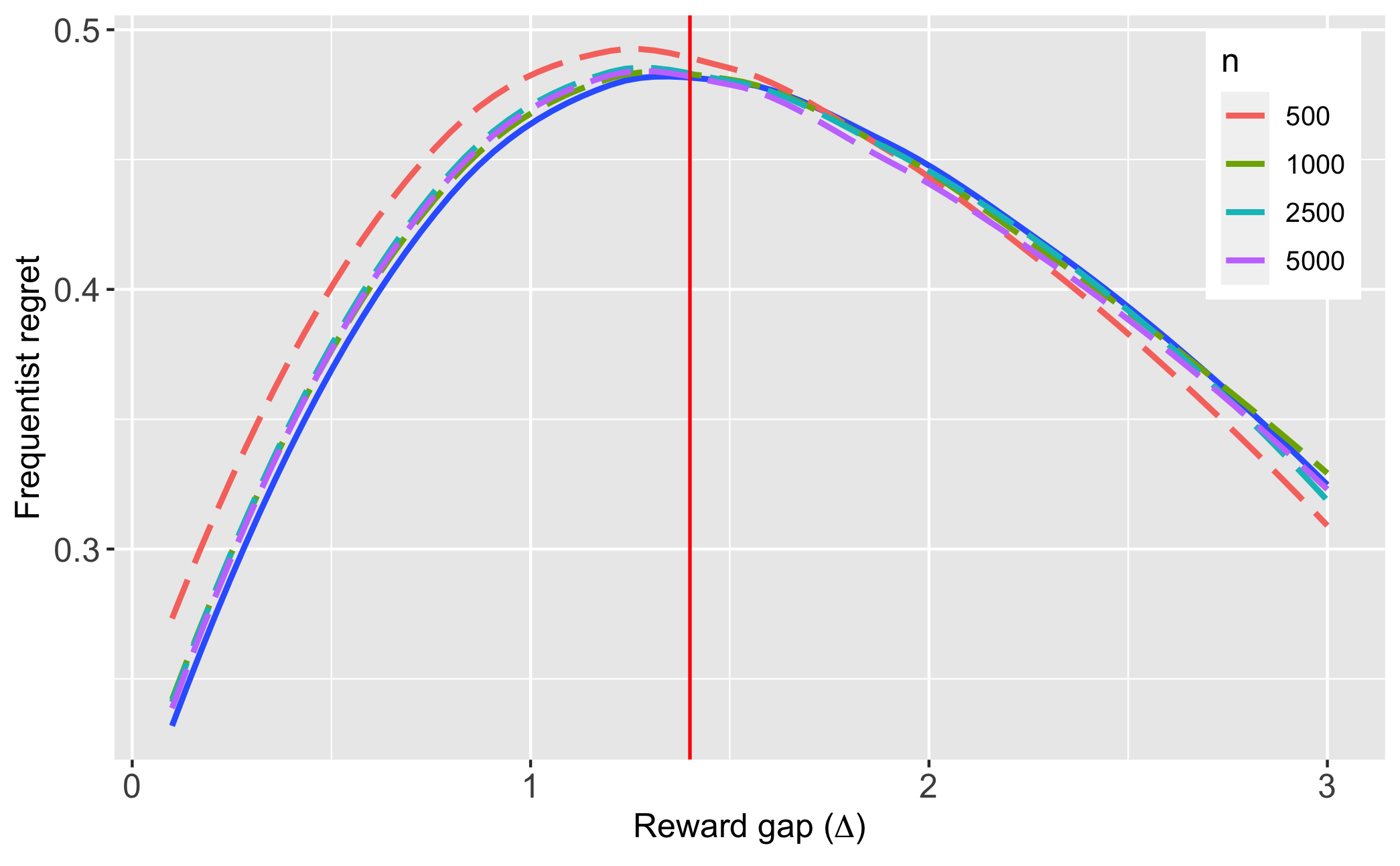
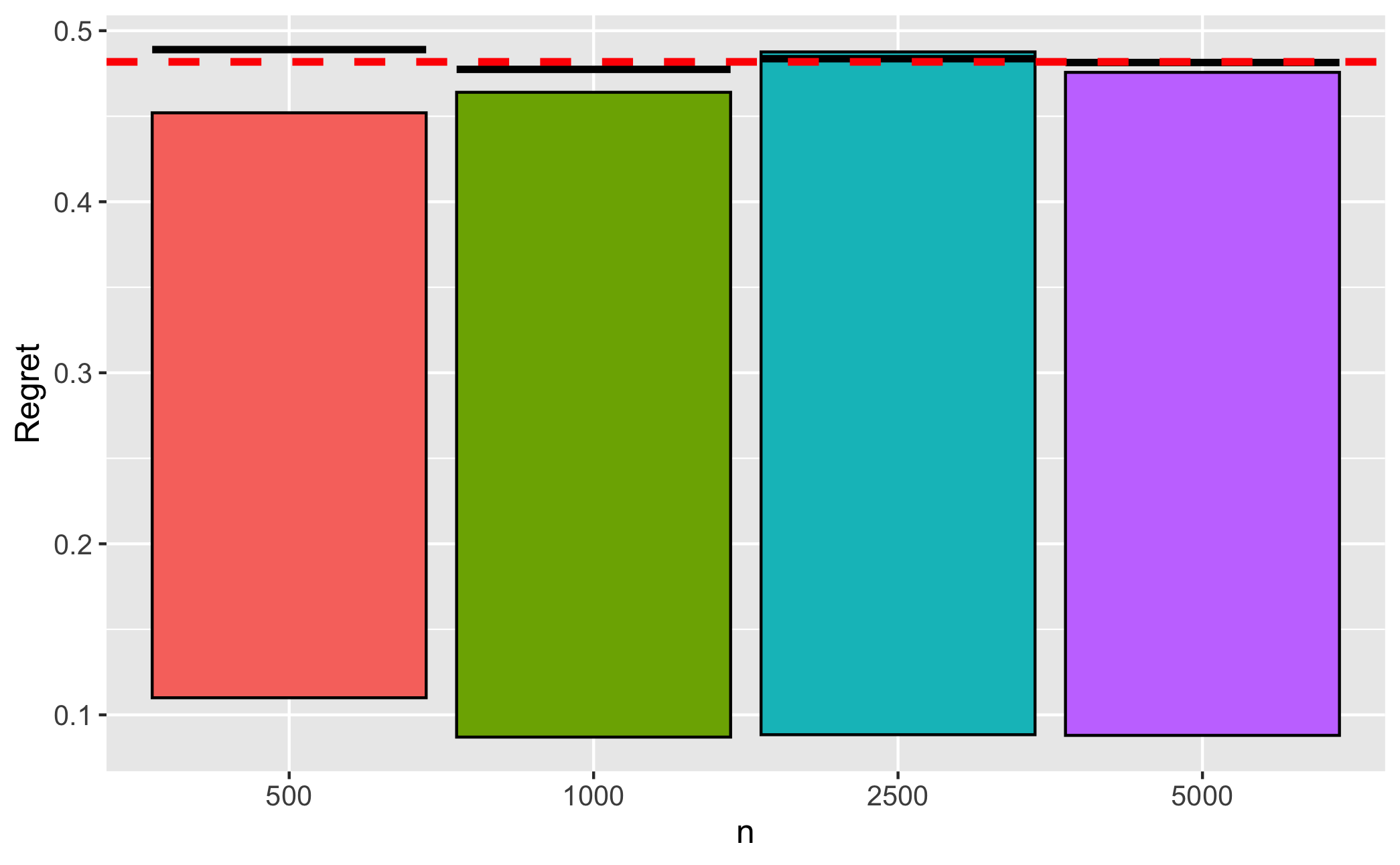
| A: Frequentist regret profiles | B: Performance under least-favorable prior |
Note: The solid curve in Panel A is the regret profile of ; the vertical red line denotes . We only plot the results for as the values are close to symmetric. The dashed red line in Panel B is , the asymptotic minimax regret. Black lines within the bars denote the Bayes regret in finite samples, under the least favorable prior. The bars describe the interquartile range of regret.
8. Conclusion
This paper proposes a minimax optimal procedure for determining the best treatment when sampling is costly. The optimal sampling rule is just the Neyman allocation, while the optimal stopping rule is time-stationary and advises that the experiment be terminated when the average difference in outcomes multiplies by the number of observations exceeds a specific threshold. While these rules were derived under diffusion asymptotics, it is shown that finite sample counterparts of these rules remain optimal under both parametric and non-parametric regimes. The form of these rules is robust to a number of different variations of the original problem, e.g., under batching, different cost functions etc. Given the simple nature of these rules, and the potential for large sample efficiency gains (requiring, on average, 40% fewer observations than standard approaches), we believe they hold a lot of promise for practical use.
The paper also raises a number of avenues for future research. While our results were derived for binary treatments, multiple treatments are common in practice, and it would be useful to derive the optimal decision rules in this setting. We do expect, however, that in this case the optimal sampling rule would no longer be fixed, but history dependent. As noted previously, our setting also does not cover discounting and asymmetric cost functions. It is hoped that the techniques developed in this paper could help answer some of these outstanding questions.
References
- Adusumilli (2021) K. Adusumilli, “Risk and optimal policies in bandit experiments,” arXiv preprint arXiv:2112.06363, 2021.
- Armstrong (2022) T. B. Armstrong, “Asymptotic efficiency bounds for a class of experimental designs,” arXiv preprint arXiv:2205.02726, 2022.
- Arrow et al. (1949) K. J. Arrow, D. Blackwell, and M. A. Girshick, “Bayes and minimax solutions of sequential decision problems,” Econometrica, pp. 213–244, 1949.
- Barles and Souganidis (1991) G. Barles and P. E. Souganidis, “Convergence of approximation schemes for fully nonlinear second order equations,” Asymptotic analysis, vol. 4, no. 3, pp. 271–283, 1991.
- Berger (2013) J. O. Berger, Statistical decision theory and Bayesian analysis. Springer Science & Business Media, 2013.
- Bertsekas (2012) D. Bertsekas, Dynamic programming and optimal control: Volume II. Athena scientific, 2012, vol. 1.
- Chernoff (1959) H. Chernoff, “Sequential design of experiments,” The Annals of Mathematical Statistics, vol. 30, no. 3, pp. 755–770, 1959.
- Chernoff and Petkau (1981) H. Chernoff and A. J. Petkau, “Sequential medical trials involving paired data,” Biometrika, vol. 68, no. 1, pp. 119–132, 1981.
- Colton (1963) T. Colton, “A model for selecting one of two medical treatments,” Journal of the American Statistical Association, vol. 58, no. 302, pp. 388–400, 1963.
- Deng et al. (2013) A. Deng, Y. Xu, R. Kohavi, and T. Walker, “Improving the sensitivity of online controlled experiments by utilizing pre-experiment data,” in Proceedings of the sixth ACM international conference on Web search and data mining, 2013, pp. 123–132.
- Fan and Glynn (2021) L. Fan and P. W. Glynn, “Diffusion approximations for thompson sampling,” arXiv preprint arXiv:2105.09232, 2021.
- Fehr and Rangel (2011) E. Fehr and A. Rangel, “Neuroeconomic foundations of economic choice–recent advances,” Journal of Economic Perspectives, vol. 25, no. 4, pp. 3–30, 2011.
- Fudenberg et al. (2018) D. Fudenberg, P. Strack, and T. Strzalecki, “Speed, accuracy, and the optimal timing of choices,” American Economic Review, vol. 108, no. 12, pp. 3651–84, 2018.
- Garivier and Kaufmann (2016) A. Garivier and E. Kaufmann, “Optimal best arm identification with fixed confidence,” in Conference on Learning Theory. PMLR, 2016, pp. 998–1027.
- Hébert and Woodford (2017) B. Hébert and M. Woodford, “Rational inattention and sequential information sampling,” National Bureau of Economic Research, Tech. Rep., 2017.
- Hirano and Porter (2009) K. Hirano and J. R. Porter, “Asymptotics for statistical treatment rules,” Econometrica, vol. 77, no. 5, pp. 1683–1701, 2009.
- Karatzas and Shreve (2012) I. Karatzas and S. Shreve, Brownian motion and stochastic calculus. Springer Science & Business Media, 2012, vol. 113.
- Lai et al. (1980) T. Lai, B. Levin, H. Robbins, and D. Siegmund, “Sequential medical trials,” Proc. Natl. Acad. Sci. U.S.A., vol. 77, no. 6, pp. 3135–3138, 1980.
- Lattimore and Szepesvári (2020) T. Lattimore and C. Szepesvári, Bandit algorithms. Cambridge University Press, 2020.
- Le Cam and Yang (2000) L. Le Cam and G. L. Yang, Asymptotics in statistics: some basic concepts. Springer Science & Business Media, 2000.
- Liang et al. (2022) A. Liang, X. Mu, and V. Syrgkanis, “Dynamically aggregating diverse information,” Econometrica, vol. 90, no. 1, pp. 47–80, 2022.
- Luce et al. (1986) R. D. Luce et al., Response times: Their role in inferring elementary mental organization. Oxford University Press on Demand, 1986, no. 8.
- Manski (2021) C. F. Manski, “Econometrics for decision making: Building foundations sketched by haavelmo and wald,” Econometrica, vol. 89, no. 6, pp. 2827–2853, 2021.
- Manski and Tetenov (2016) C. F. Manski and A. Tetenov, “Sufficient trial size to inform clinical practice,” Proc. Natl. Acad. Sci. U.S.A., vol. 113, no. 38, pp. 10 518–10 523, 2016.
- Morris and Strack (2019) S. Morris and P. Strack, “The wald problem and the relation of sequential sampling and ex-ante information costs,” Available at SSRN 2991567, 2019.
- Øksendal (2003) B. Øksendal, “Stochastic differential equations,” in Stochastic differential equations. Springer, 2003, pp. 65–84.
- Qin and Russo (2022) C. Qin and D. Russo, “Adaptivity and confounding in multi-armed bandit experiments,” arXiv preprint arXiv:2202.09036, 2022.
- Qin et al. (2017) C. Qin, D. Klabjan, and D. Russo, “Improving the expected improvement algorithm,” Advances in Neural Information Processing Systems, vol. 30, 2017.
- Ratcliff and McKoon (2008) R. Ratcliff and G. McKoon, “The diffusion decision model: theory and data for two-choice decision tasks,” Neural computation, vol. 20, no. 4, pp. 873–922, 2008.
- Reikvam (1998) K. Reikvam, “Viscosity solutions of optimal stopping problems,” Stochastics and Stochastic Reports, vol. 62, no. 3-4, pp. 285–301, 1998.
- Shiryaev (2007) A. N. Shiryaev, Optimal stopping rules. Springer Science & Business Media, 2007.
- Sims (2003) C. A. Sims, “Implications of rational inattention,” Journal of monetary Economics, vol. 50, no. 3, pp. 665–690, 2003.
- Sion (1958) M. Sion, “On general minimax theorems.” Pacific Journal of mathematics, vol. 8, no. 1, pp. 171–176, 1958.
- US Food and Drug Admin. (2018) US Food and Drug Admin., “FDA In Brief: FDA launches new pilot to advance innovative clinical trial designs as part agency’s broader program to modernize drug development and promote innovation in drugs targeted to unmet needs,” 2018. [Online]. Available: "https://www.fda.gov/news-events/fda-brief/fda-brief-fda-modernizes-clinical-trial-designs-and-approaches-drug-development-proposing-new"
- Van der Vaart (2000) A. W. Van der Vaart, Asymptotic statistics. Cambridge university press, 2000.
- Van Der Vaart and Wellner (1996) A. W. Van Der Vaart and J. Wellner, Weak convergence and empirical processes: with applications to statistics. Springer Science & Business Media, 1996.
- Wager and Xu (2021) S. Wager and K. Xu, “Diffusion asymptotics for sequential experiments,” arXiv preprint arXiv:2101.09855, 2021.
- Wald (1945) A. Wald, “Statistical decision functions which minimize the maximum risk,” Annals of Mathematics, pp. 265–280, 1945.
- Wald (1947) ——, “Sequential analysis,” Tech. Rep., 1947.
- Zaks (2020) T. Zaks, “A phase 3, randomized, stratified, observer-blind, placebo-controlled study to evaluate the efficacy, safety, and immunogenicity of mrna-1273 sars-cov-2 vaccine in adults aged 18 years and older,” Protocol Number mRNA-1273-P301. ModernaTX (20 August 2020) https://www. modernatx. com/sites/default/files/mRNA-1273-P301-Protocol. pdf, 2020.
Appendix A Proofs
A.1. Proof of Theorem 1
The proof makes use of the following lemmas:
Lemma 1.
Suppose nature sets to be a symmetric two-point prior supported on ). Then the decision , where is defined in (A.3), is a best response by the DM.
Proof.
The prior is an indifference-inducing one, so by the argument given in Section 3.1, the DM is indifferent between any sampling rule . Thus, is a best-response to this prior. Also, the prior is symmetric with , so by (2.5), the Bayes optimal implementation rule is
It remains to compute the Bayes optimal stopping time. Let denote the state when the prior is , with otherwise. The discussion in Section 3.1 implies that, conditional on , the likelihood ratio process does not depend on and evolves as
where is one-dimensional Brownian motion. By a similar argument as in Shiryaev (2007, Section 4.2.1), this in turn implies that the posterior probability is also independent of and evolves as
Therefore, by (2.7) the optimal stopping time also does not depend on and is given by
| (A.1) | ||||
| (A.2) |
Inspection of the objective function in (A.1) shows that this is exactly the same objective as in the Bayesian hypothesis testing problem, analyzed previously by Arrow et al. (1949) and Morris and Strack (2019). We follow the analysis of the latter paper. Morris and Strack (2019) show that instead of choosing the stopping time , it is equivalent to imagine that the DM chooses a probability distribution over the posterior beliefs at an ‘ex-ante’ cost
subject to the constraint . Under the distribution , the expected regret, exclusive of sampling costs, for the DM is
Hence, the stopping time, , that solves (A.1) is the one that induces the distribution , defined as
where
Clearly, . Hence, setting
it is easy to see that is a two-point distribution, supported on with equal probability . By Shiryaev (2007, Section 4.2.1), this distribution is induced by the stopping time , where
| (A.3) |
Hence, this stopping time is the best response to nature’s prior. ∎
Lemma 2.
Suppose is such that . Then, for any ,
Thus, the frequentist regret of depends on only through .
Proof.
Suppose that . Define
Note that under and ,
where is one-dimensional Brownian motion. Hence We can write the stopping time in terms of as
and the implementation rule as
Now, noting the form of , we can apply similar arguments as in Shiryaev (2007, Section 4.2, Lemma 5), to show that
Furthermore, following Shiryaev (2007, Section 4.2, Lemma 4), we also have
Hence, the frequentist regret is given by
While the above was shown under , an analogous argument under gives the same expression for . ∎
Lemma 3.
Consider a two-player zero-sum game in which nature chooses a symmetric two-point prior supported on and for some and the DM chooses for some . There exists a unique Nash equilibrium to this game at and , where are defined in Section 3.
Proof.
Let be the symmetric two-point prior supported on and . By Lemma 2, the frequentist regret under a given choice of and is given by , where
Lemma 2 further implies that the frequentist regret depends on only through . Therefore, the frequentist regret under both support points of must be the same. Hence, the Bayes regret, , is the same as the frequentist regret at each support point, i.e.,
| (A.4) |
We aim to find a Nash equilibrium in a two-player game in which natures chooses , equivalently , to maximize , while the DM chooses , equivalently , to minimize .
For , the unique Nash equilibrium to this game is given by and . We start by first demonstrating the existence of a unique Nash equilibrium. This is guaranteed by Sion’s minimax theorem (Sion, 1958) as long as is continuous in both arguments (which is easily verified), and ‘convex quasi-concave’ on .101010In fact, convexity can be replaced with quasi-convexity for the theorem. To show convexity in the first argument, write where
Now, for any fixed , it is easy to verify that and are convex over the domain . Since the composition of convex functions is also convex, this proves convexity of . To prove is quasi-concave, write , where
Now, and are concave over , so is also concave over for any fixed . Concavity implies the level set is a closed interval in for any . But is positive and strictly decreasing, so for a fixed ,
is also a closed interval in , and therefore, convex, for any . This proves quasi-concavity of whenever . At the same time, when ; hence, is in fact quasi-concave for any . We thus conclude by Sion’s theorem that the Nash equilibrium exists and is unique. It is then routine to numerically compute though first-order conditions; we skip these calculations, which are straightforward. Figure A.1 provides a graphical illustration of the Nash equilibrium.
It remains to determine the Nash equilibrium under general . By the form of , if is a best response to for , then is a best response to for general . Similarly, if is a best response to for , then is a best response to for general . This proves and is a Nash equilibrium in the general case. ∎
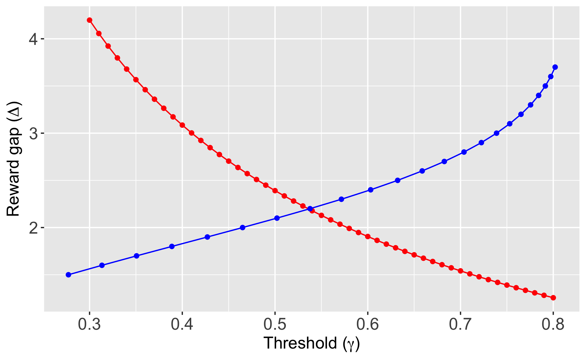
Note: The red curve describes the best response of to a given , while the blue curve describes the best response of to a given . The point of intersection is the Nash equilibrium. This is for .
We now complete the proof of Theorem 1: By Lemma 1, is the optimal Bayes decision corresponding to . We now show
| (A.5) |
which implies is minimax optimal according to the verification theorem in Berger (2013, Theorem 17). To this end, recall from Lemma 2 that the frequentist regret depends on only through . Furthermore, by Lemma 3, is the best response of nature to . These results imply
A.2. Proof of Corollary 1
We employ the same strategy as in the proof of Theorem 1. Suppose nature employs the indifference prior , for any . Then by similar arguments as earlier, the DM is indifferent between any sampling rule , and the optimal implementation rule is
We now determine Nature’s best response to the DM choosing , where is the Neyman allocation. Consider an arbitrary such that . Suppose . Under ,
where is the standard Weiner process, so the expected regret under is
| (A.6) |
An analogous argument shows that the same expression holds when as well. Consequently, nature’s optimal choice of is to set to , but is otherwise indifferent between any such that . Thus, is a best response by nature to the DM’s choice of .
We have thereby shown form a Nash equilibrium. That is minimax optimal then follows by similar arguments as in the proof of Theorem 1.
A.3. Proof of Theorem 2
Our aim is to show (4.3). The outline of the proof is as follows: First, as in Adusumilli (2021), we replace the true marginal and posterior distributions with suitable approximations. Next, we apply dynamic programming arguments and viscosity solution techniques to obtain a HJB-variational inequality (HJB-VI) for the value function in the experiment. Finally, the HJB-VI is connected to the problem of determining the optimal stopping time under diffusion asymptotics.
Step 0 (Definitions and preliminary observations)
Under , let denote the state and the state . Also, let denote the stacked representation of outcomes from the first observations corresponding to treatment , and for any , take to be the distribution corresponding to the joint density , where
Also, define as the marginal distribution of , i.e., it is the probability measure whose density, with respect to the dominating measure , is
Due to the two-point support of , the posterior density can be associated with a scalar,
That the posterior depends on only via is an immediate consequence of Adusumilli (2021, Lemma 1). Recalling the definition of in (4.2), we have , where, for any ,
The first equation above always holds, while the second holds under the simplification described in Section 4.
Let
| (A.7) |
denote the (standardized) score process. Under quadratic mean differentiability - Assumption 1(i) - the following SLAN property holds for both treatments:
| (A.8) |
See Adusumilli (2021, Lemma 2) for the proof.111111It should be noted that the score process in that paper is defined slightly differently, as under the present notation.
As in Adusumilli (2021), we now define approximate versions of the true marginal and posterior by replacing the actual likelihood with
| (A.9) |
In other words, we approximate the true likelihood with the first two terms in the SLAN expansion (A.8).
(Approximate marginal:) Denote by the measure whose density is , and take to be its marginal over given the prior . Note that the density (wrt ) of is
| (A.10) |
Also, define . Then, approximates the true marginal .
(Approximate posterior:) Next, let be the approximate likelihood ratio
where
| (A.11) |
Based on the above, an approximation to the true posterior is given by121212Formally, this follows by the disintegration of measure, see, e.g., Adusumilli (2021, p.17).
| (A.12) |
where for . When , the approximate posterior in turn implies an approximate posterior, , over that takes the value with probability and with probability .
Step 1 (Posterior and probability approximations)
Set . Using dynamic programming arguments, it is straightforward to show that there exists a non-randomized sampling rule and stopping time that minimizes for any prior . We therefore restrict to the set of all deterministic rules, . Under deterministic policies, the sampling rules , states and stopping times are all deterministic functions of . Recall that are the stacked vector of outcomes under observations of each treatment. It is useful to think of as quantities mapping to realizations of regret.131313Note that still need to satisfy the measurability restrictions, and some components of may not be observed as both treatments cannot be sampled times. Taking to be the expectation under , we then have
for any deterministic .
Step 2 (Recursive formula for )
We now employ dynamic programming arguments to obtain a recursion for . This requires a bit of care since is not a probability, even though it does integrate to 1 asymptotically.
Recall that is the probability measure on that assigns probability to and probability to . Define
| (A.14) |
where . In words, is the approximate probability density over the future values of the stacked rewards given the current state . Note that, is the normalization constant of .
By Lemma 8 in Appendix B.6, , where solves the recursion
| (A.15) |
for , and
The function accounts for the fact is not a probability.
Now, Lemma 9 in Appendix B.6 shows that
| (A.16) |
for some and any . Furthermore, by Assumption 1(iii),
| (A.17) |
where . Since is uniformly bounded, it follows from (A.17) that is also uniformly bounded. Then, (A.16) and (A.17) imply
where is defined as the solution to the recursion
| (A.18) | ||||
We can drop the state variables in as they enter the definition of only via , which was shown in (A.16) to be uniformly close to 1.
Step 3 (PDE approximation and relationship to optimal stopping)
For any , let
Lemma 10 in Appendix B.6 shows that converges locally uniformly to , the unique viscosity solution of the HJB-VI
| (A.19) |
Note that the sampling rule does not enter the HJB-VI. This is a consequence of the choice of the prior, .
There is a well known connection between HJB-VIs and the problem of optimal stopping that goes by the name of smooth-pasting or the high contact principle, see Øksendal (2003, Chapter 10) for an overview. In the present context, letting denote one-dimensional Brownian motion, it follows by Reikvam (1998) that
and is the set of all stopping times adapted to the filtration generated by .
Step 4 (Taking )
Through steps 1-3, we have shown
We now argue that
Suppose not: Then, there exists , and some stopping time such that for all (note that we always have by definition). Now, is uniformly bounded, so by the dominated convergence theorem, . Hence,
This is a contradiction.
A.4. Proof of Theorem 3
For any , let denote the joint distribution with density . Take to be the corresponding expectation. We can write as
Define , and . In addition, we also define .
Step 1 (Weak convergence of )
Denote By the SLAN property (A.8), independence of given , and the central limit theorem,
| (A.20) | ||||
| (A.21) |
Therefore, by Le Cam’s first lemma, and are mutually contiguous.
We now determine the distribution of . We start by showing
| (A.22) |
uniformly over . Choose any . For , we must have , so (A.22) follows from Assumption 1(ii), which implies
| (A.23) |
As for the other values of , by (4.4) and (A.23),
uniformly over .
Now, (A.22) implies
| (A.24) |
By Donsker’s theorem, and recalling that ,
where can be taken to be independent Weiner processes due to the independence of under . Combined with (A.24), we conclude
| (A.25) |
where is another Weiner process.
Let denote the normal random variable in (A.21). Equations (A.21) and (A.25) imply that are asymptotically tight, and therefore, the joint is also asymptotically tight under Furthermore, for any , it can be shown using (A.24) and (A.20) that
Based on the above, an application of Le Cam’s third lemma as in Van Der Vaart and Wellner (1996, Theorem 3.10.12) then gives
| (A.26) |
Step 2 (Weak convergence of )
Let denote the metric space of all functions from to equipped with the sup norm. For any element , define and .
Now, under , is the Weiner process, whose sample paths take values (with probability 1) in , the set of all continuous functions such that are regular points (i.e., if , changes sign infinitely often in any time interval , ; a similar property holds under ). The latter is a well known property of Brownian motion, see Karatzas and Shreve (2012, Problem 2.7.18), and it implies must ‘cross’ the boundary within an arbitrarily small time interval after hitting or . It is then easy to verify that if with for all and , then and . By construction, and , so by (A.25) and the extended continuous mapping theorem (Van Der Vaart and Wellner, 1996, Theorem 1.11.1)
where and .
For general , is distributed as in (A.26). By the Girsanov theorem, the probability law induced on by the process is absolutely continuous with respect to the probability law induced by . Hence, with probability 1, the sample paths of again lie in . Then, by similar arguments as in the case with , but now using (A.26), we conclude
| (A.27) |
Step 3 (Convergence of )
From (3.5) and the discussion in Section 3.1, it is clear that the distribution of is the same as that of in the diffusion regime. Thus, the joint distribution, , of , defined in Step 2, is the same as the joint distribution of
in the diffusion regime, when the optimal sampling rule is used. Therefore, defining and to be the expectation under , we obtain
where denotes the frequentist regret of in the diffusion regime. Now, recall that by the definitions stated early on in this proof,
Since are bounded and by Assumption 1(iii), it follows from (A.27) that for each ,
| (A.28) |
For any given and , a dominated convergence argument as in Step 4 of the proof of Theorem 2 shows that there exists large enough such that
| (A.29) |
for all . Fix a finite subset of and define Then, (A.28) and (A.29) imply
for all . Since the above is true for any and ,
The inequality can be made an equality due to Theorem 2. We have thereby proved Theorem 3.
ONLINE APPENDIX
Appendix B Supplementary results
B.1. Proof of equation (3.7)
We exploit the fact that the least favorable prior has a two point support, and that the reward gap is the same under both support points. Fix some values of . Recall the definition of as the probability of mis-identification error from (3.6), and observe that . Furthermore, by Lemma 2,
where the second equality follows from the expression for in (3.6).
Let denote the state when and the state when . Because of the nature of the prior, we can think of a non-sequential experiment as choosing a set of mis-identification probabilities under the two states (e.g., is the probability of choosing treatment 0 under ), along with a duration (i.e., a sample size), . To achieve a Bayes regret of , we would need . For any , let denote the minimum duration of time needed to achieve these mis-identification probabilities. Following Shiryaev (2007, Section 4.2.5), we have
Hence,
It can be seen that the minimum is reached when , and we thus obtain
Therefore,
B.2. Proof sketch of Theorem 5
For any , , let denote the joint distribution . Take to be the corresponding expectation. As in Section 5, we can associate each with an element from the space of square integrable sequences . In what follows, we write , and define and .
We only rework the first step of the proof of Theorem 3 as the remaining steps can be applied with minor changes.
Denote . By the SLAN property (5.2), independence of given , and the central limit theorem,
| (B.1) |
Therefore, by Le Cam’s first lemma, and are mutually contiguous. Next, define
By similar arguments as in the proof of Theorem 3,
| (B.2) |
Then, by Donsker’s theorem, and recalling that , we obtain
where can be taken to be independent Weiner processes due to the independence of under . Combined with (B.2), we conclude
| (B.3) |
where is another Weiner process.
Equations (B.1) and (B.3) imply that are asymptotically tight, and therefore, the joint is also asymptotically tight under It remains to determine the point-wise distributional limit of for each . By our representation of , we have , where is orthogonal to the influence function . This implies , and therefore, after some straightforward algebra exploiting the fact that are independent iid sequences, we obtain
Combining the above with (B.2) and the first line of (B.1), we find
for each , where the last step makes use of the independence of and . Based on the above, an application of Le Cam’s third lemma as in Van Der Vaart and Wellner (1996, Theorem 3.10.12) then gives
| (B.4) |
B.3. Alternative cost functions
We follow the basic outline of Section 3.1 and Lemmas 1-3. Our ansatz is that the least favorable prior should be within the class of indifference priors, , and the minimax decision rule should lie within the class .
The DM’s response to .
Suppose nature employs the indifference prior . Then it is clear from the discussion in Section 3.1, and the symmetry of the sampling costs that the DM is indifferent between any sampling rule, and the Bayes optimal implementation rule is . To determine the Bayes optimal stopping rule, we employ a similar analysis as in Lemma 1. Define
Note that is the sampling cost in terms of the posterior probability , as . Let denote the expectation over given the prior and sampling rule . By Morris and Strack (2019, Proposition 2),
where is the distribution induced over by the stopping time . Hence, as in Lemma 1, we can suppose that instead of choosing , the DM chooses a probability distribution over the posterior beliefs at an ‘ex-ante’ cost
subject to the constraint . Hence, the Bayes optimal stopping time is the one that induces the distribution , defined as
As , cannot be minimized at . Consider, then, for . In this region, , where by the assumption . This proves is convex in . Also, , and under the assumption , it is easy to see that as , with monotonically decreasing on . Taken together, these results imply has a unique minimum in . Denote By the symmetry of sampling costs, , and so the global minima of are . Given the constraint , we conclude that is a two-point distribution, supported on with equal probability . By Shiryaev (2007, Section 4.2.1), this distribution is induced by the stopping time , where
This stopping time is the best response to nature’s prior .
Nature’s response to .
We will determine nature’s best response to the DM choosing by obtaining a formula for the frequentist regret . Denote , and take to be the solution of the ODE
It is easy to show that the solution is
In what follows we write .
We now claim that for any stopping time, ,
| (B.5) |
To prove the above, we start by recalling from (3.5) that
where is a one-dimensional Weiner process. Then, for any bounded stopping time , Ito’s lemma implies
where the last step follows from the definition of . This proves (B.5) for bounded stopping times. The extension to unbounded stopping times follows by a similar argument as in the proof of Proposition 2 in Morris and Strack (2019).
Nash equilibrium.
By similar arguments as in the proof of Theorem 1, the Nash equilibrium is given by where is the solution to the minimax problem
B.4. Analysis of other regret measures
Following the discussion in Section 6.4, suppose that we measure regret in the implementation phase using some nonlinear functional of the outcome distributions . We assume that is a regular functional of the data, i.e., for each , there is a such that
| (B.8) |
for each of the sub-models introduced in Section 5.141414Following Van der Vaart (2000, Section 25.3), we may restrict attention to those for which the Hadamard derivative of , as given by (B.8), exists. The function is termed the efficient influence function.
Define . It is possible to select in such a manner that is a set of orthonormal basis functions for the closure of . We can also choose these bases so they lie in , i.e., for all . By the Hilbert space isometry, each is then associated with an element from the space of square integrable sequences, , where and for all .
Note that the above setup closely mirrors the discussion in Section 5. Indeed, when is the mean functional, the efficient influence function is just , as defined in that section. It is then easy to verify that the derivation of the minimax lower bound in Theorem 4, and the discussion preceding it, goes through unchanged even for general functionals.
For decision rules that attain the lower bound, consider , as defined in Section 4.3, but with in (5.4) now representing the efficient influence function process for treatment , i.e.,
and . By the same method of proof as in Section B.2, it is easy to see that attains the lower bound and Theorem 5 thereby applies to general functionals as well.
B.5. Additional simulations
B.5.1. Updating using a prior
As noted in Section 6.3, instead of using forced sampling to estimate the values of , we could instead employ a prior and continuously update these parameter values. Here, we report simulation results from using this approach in the context of the numerical illustration from Section 7.
Since the outcome model is Bernoulli, we employ a beta prior over the unknown quantities . The prior parameters are taken to be ; these imply that the prior is centered around . We then apply our proposed policies while continuously updating the values of using the posterior means of . We experimented with alternative prior parameters, but they did not change the results substantively.
Figure B.2, Panel A plots the finite sample frequentist regret profile of (i.e., with ) for various values of , along with that of under diffusion asymptotics. The approach of using the prior performs substantially worse than forced sampling (as can be seen by comparing the figure to Figure 7.1), with the performance being worse for higher values of . It appears that continuously updating the prior results in more variability, leading to higher expected regret than that under the minimax policy (for large ). However, the minimax regret itself is actually close to the asymptotic value, as can be seen by comparing the maximum values of the regret profiles; in particular, the difference is less than 3%. Nevertheless, we recommend employing forced sampling in practice, at-least for Bernoulli outcomes, as it has a strong theoretical justification.
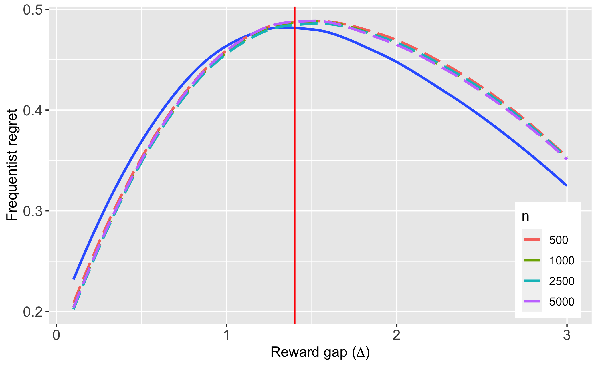
Note: The solid curve is the regret profile of ; the vertical red line denotes . We only plot the results for as the values are close to symmetric.
B.5.2. Simulations using Gaussian outcomes
To assess the finite sample performance of the proposed policies under continuous outcomes, we ran additional Monte-Carlo simulations assuming Gaussian outcomes for each treatment. This is a parametric setting in which has the form
Figure B.2, Panel A plots the finite sample frequentist regret profile of (i.e., with ) for various values of , along with that of under diffusion asymptotics. The parameter values are and . Given these parameter values, each corresponds to a sampling cost of . It is seen that diffusion asymptotics provide a very good approximation to the finite sample properties of , even for such relatively small values of as . Furthermore, can be seen to attain the lower bound for minimax regret. Panel B of the same figure displays some summary statistics for Bayes regret under when nature chooses the least favorable prior, . The finite sample expected regret is very close to , the value of minimax regret under diffusion asymptotics. We can also infer that the distribution of regret under is positively skewed and heavy tailed.
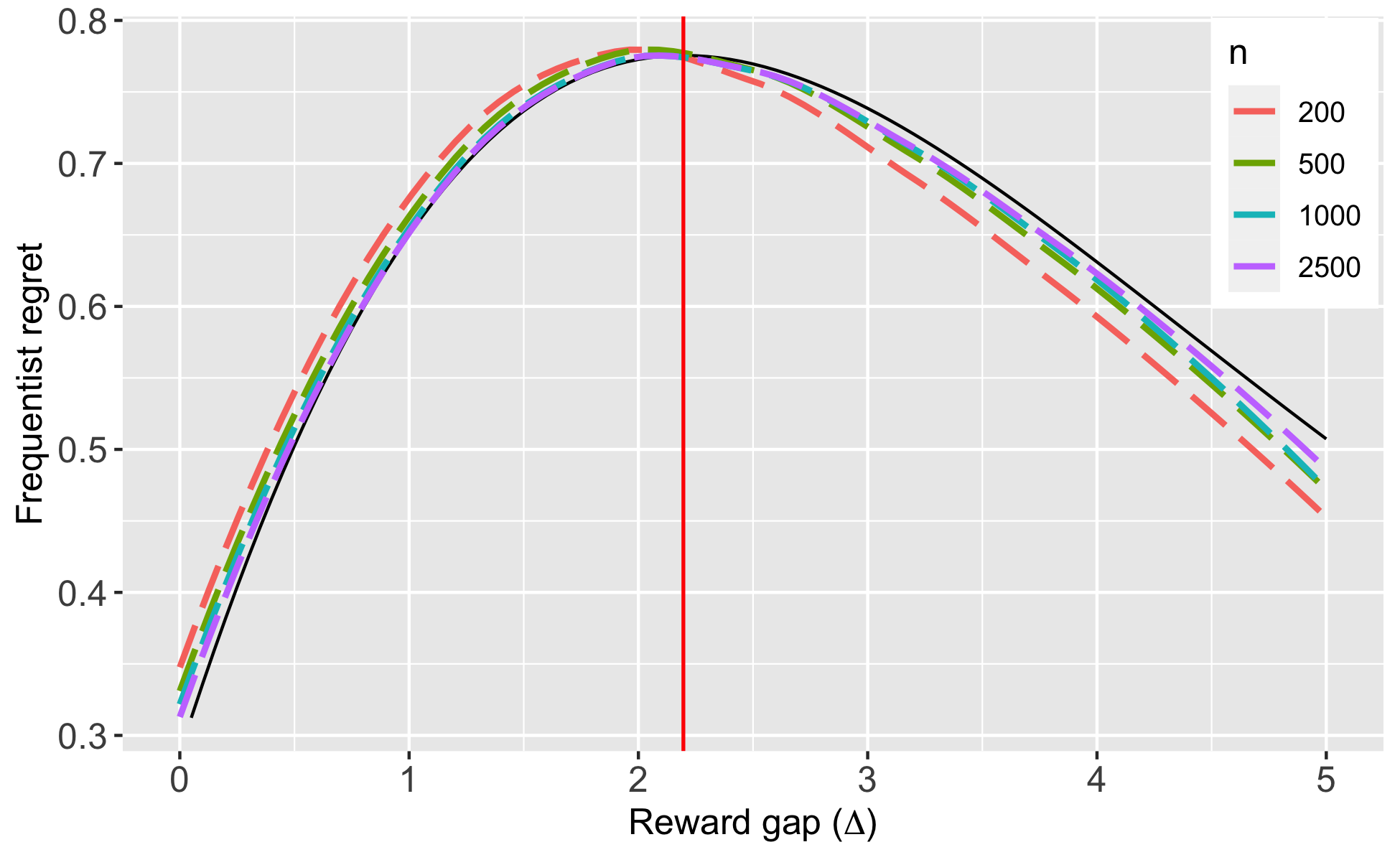
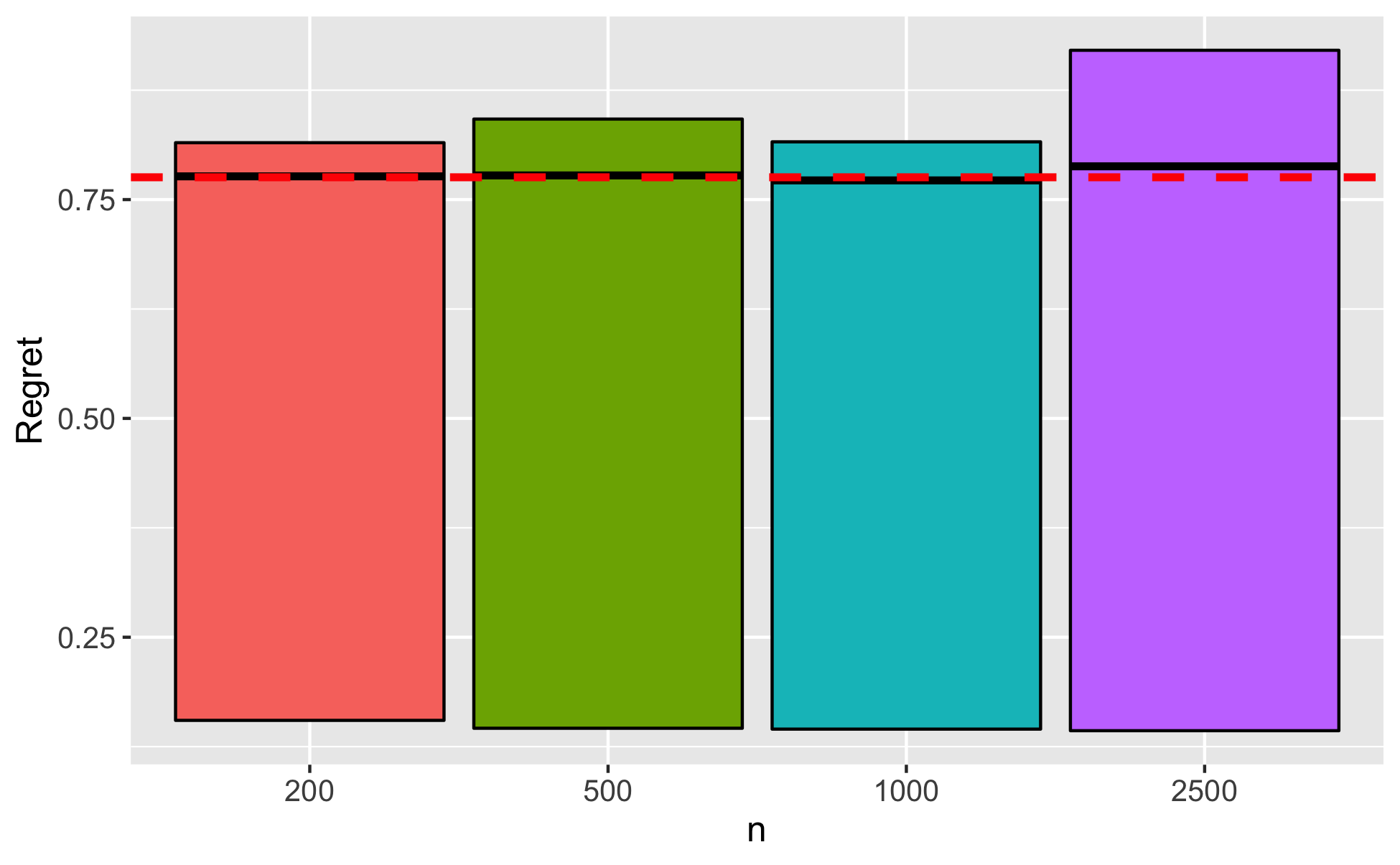
| A: Frequentist regret profiles | B: Performance under least-favorable prior |
Note: The solid curve in Panel A is the regret profile of ; the vertical red line denotes . We only plot the results for as the values are close to symmetric. The dashed red line in Panel B is , the asymptotic minimax regret. Black lines within the bars denote the Bayes regret in finite samples, under the least favorable prior. The bars describe the interquartile range of regret. Parameter values are , .
B.6. Supporting lemmas for the proof of Theorem 2
We suppose that Assumption 1 holds for all the results in this section. We also make heavy use of the notation defined in Appendix A.3. Additionally, for some , define
Lemma 4.
For any , there exist such that and implies . Furthermore, letting denote the expectation under ,
Proof.
The proof follows the same outline as in Adusumilli (2021, Lemma 3). Set
Note that is a partial sum process with mean under . By Kolmogorov’s maximal inequality and Assumption 1(ii), for each ,
Since are independent, it follows that for any . But by (A.8) and standard arguments involving Le Cam’s first lemma, is contiguous to for all . This implies is also contiguous to (this can be shown using the dominated convergence theorem; see also, Le Cam and Yang, p.138). Consequently, for any . The first claim is a straightforward consequence of this.
We now prove the second claim: For any , recall that denotes the probability measure over defined as
Now, by similar arguments as in Adusumilli (2021, Lemma 3), is contiguous to for any and deterministic sequence converging to some . Due to the independence of for any , it then follows that is contiguous to .
Now, let denote quantities such that
for some arbitrarily small (this is always possible by the definition of the supremum). Without loss of generality, we may assume converges to some ; otherwise we can employ a subsequence argument since lie in a bounded set. Define
The claim follows if we show . By Lemma A.8 and the definition of ,
where under for each . Since
is bounded for any fixed by the definition of , this implies under . Next, we argue is uniformly integrable. The first term
in the definition of is bounded, and therefore uniformly integrable, for any . It remains to prove uniform integrability of
For any ,
But,
so the contiguity of with respect to implies we can choose and large enough such that
for any arbitrarily small . These results demonstrate uniform integrability of under . Since convergence in probability implies convergence in expectation for uniformly integrable random variables, we have thus shown , which concludes the proof. ∎
Lemma 5.
For any measure , define as the restriction of to the set . Then, , where denotes the total-variation metric.
Proof.
Denote . By the properties of the total variation metric, contiguity of with respect to (shown in the proof of Lemma 4) and the absolute continuity of with respect to (by construction),
In the last expression, denote the term within the brackets by . By Lemma 4, for each . Since is a two-point prior, this proves the desired claim. ∎
Lemma 6.
.
Proof.
Define
We can then write
Recall the definition of in (A.12) and note that is bounded under the set . Then, by the SLAN property (A.8) and some straightforward algebra,
Due to the continuous mapping theorem, the above in turn implies
But it was shown in the proof of Lemma 4 that is contiguous with respect to ; hence,
Since both , the claim follows from the dominated convergence theorem. ∎
Lemma 7.
Proof.
We prove the claim by bounding each term in the following expansion:
| (B.9) |
First, observe that by Assumption 1(iii),
| (B.10) |
where . Since is uniformly bounded, it follows from (B.10) that is also uniformly bounded. Furthermore, is also bounded. We thus conclude that and are uniformly bounded by some (suitably large) constant . The first two quantities in (B.9) are therefore bounded by and .
By Lemma 4, can be made arbitrarily small by choosing a suitably large in the definition of . Hence the first term in (B.9) converges to as .
Lemma 8.
Proof.
In what follows, we define .
Step 1 (Disintegration of ). We start by presenting a disintegration result for ; this will turn out to be convenient when applying a dynamic programming argument on . Recall the definitions of and from Step 0 of the proof of Theorem 2. Also, let
denote the joint probability density (wrt ) over and take to be the corresponding probability measure. By the disintegration theorem and the definition of , we have
| (B.11) |
Note that in the above is a function of - it is defined in (A.11) - but we have elected to suppress this dependence.
Now, can be written as
| (B.12) |
Hence, for any ,
where the first equality is a consequence of (B.12) and the definition of , and the second equality follows from (B.11). Integrating with respect to the dominating measure, , on both sides of the expression then gives (the quantity is defined in A.14)151515Recall that is some dominating measure for the prior . Here, it can be taken to be the counting measure on and .
| (B.13) |
Step 2 (Relating successive values of ). The quantity specifies the density of the unobserved elements, , of when the current state is . In this step, we aim to characterize the density of the remaining elements of , if starting from the state , we assign treatment and observe the first element, , of .
We start by noting that (B.11), (B.13) are valid for any , as long as . Suppose treatment is employed when the current state . Then, it is easily verified that
where the last equality follows from (B.11). Integrating with respect to on both sides then gives161616The quantity is defined in Step 2 of the proof of Theorem 2.
| (B.14) |
Applying (B.13) twice, with the values and , and making use of (B.14) together with the definition of from (A.11), we conclude
| (B.15) |
where . Analogously,
| (B.16) |
with now being .
Step 3 (Recursive expression for ). Let denote the value of at period . Suppose that at period of the experiment, the state is . The posterior, provides the density of the remaining elements of the vector . By extension, we may define as the density induced over paths given the knowledge of . This density consists of a point mass for , with the rest of the components of the vector distributed as .
Let and take to be the set of all possible decision rules starting from period with the usual measurability restrictions, i.e., is measurable, the stopping time is sequentially measurable, and the implementation rule is measurable. Recalling that , define
| (B.17) |
with the convention that at ,
The quantity is akin to the value function at period . Note also that the quantities in (B.17) are functions of .
Clearly, by definition, so the claim follows if we show: (i) , i.e., it is function only of ; and (ii) it satisfies the recursion (A.15). To show this, we adopt the usual approach in dynamic programming of using backward induction.
First, we argue that the induction hypothesis holds at (corresponding to ). Indeed,
and we can therefore write as a function only of .
Now suppose that the induction hypothesis holds for the periods . Consider the various possibilities at period . If the experiment is stopped right away, the continuation value of this choice is
On the other hand, if the experiment is continued and treatment 1 is sampled, the resulting continuation value is
where and . The first equality follows from (B.15), the second follows from a suitable measurable selection theorem (see, e.g., Bertsekas, 2012, Proposition A.5), the third from the definition of , and the last equality from the induction hypothesis. In a similar vein, if treatment were sampled, we would have
Now,
| (B.18) |
We have shown above that each of the three terms within the minimum in (B.18) are functions only of . Hence, . Furthermore, by the expressions for these quantities, it is clear that (B.18) is none other than (A.15). This proves the induction hypothesis for period . The claim follows. ∎
Lemma 9.
There exist non-random constants, and such that .
Proof.
Denote
and taken to be the expectation corresponding to . Then, writing the inner integral (within the brackets) in (B.19) as , we find
| (B.20) |
Since is the score function at , and . Using these results, and noting that the support of is only with due to the form of the prior, some straightforward algebra implies
Here, denotes the minimum eigenvalue of . Next, we can expand as:
| (B.21) |
Since and , the first term in (B.21) is bounded by over . Furthermore, for large enough , the second term in (B.21) is bounded by for any . Hence, setting gives . Combining the above, we conclude there exists some non-random such that
Substituting the above bound on into (B.19) gives
for some . Since we can choose any , it follows and the claim follows. ∎
Lemma 10.
Proof.
The proof consists of two steps. In the first step, we derive some preliminary results for expectations under the posterior . Then, we use the abstract convergence result of Barles and Souganidis (1991) to show that converges locally uniformly to the viscosity solution of (A.19).
Step 1 (Some results on moments of ). Let denote the expectation under . In this step, we show that there exists independent of and such that
| (B.22) | ||||
| (B.23) |
Furthermore,
| (B.24) |
Start with (B.22). Suppose . By the definition of ,
Hence,
Now, for each , define
Then,
Now, and . Hence, the first term in the above expression equals . As for the second term,
| (B.25) |
Since with , and , the first term in in (B.25) is bounded by . The second term in (B.25) is bounded by for any . Hence, setting gives
Combining the above results, we obtain
where , and the last equality follows from the definition of . In a similar manner, we can show for that
This proves (B.22).
Step 2 (Convergence to the HJB-VI). We now make the time change . Let and . Also, denote the state variables by and take to the domain of . Finally, let denote the set of all infinitely differentiable functions such that for some (such functions are also known as test functions).
Following the time change, we can alternatively represent the solution, , to (A.18) as solving the approximation scheme171717This alternative representation does not follow from an algebraic manipulation, but can be verified by checking that the relevant inequalities are preserved, e.g., implies , etc.
| (B.26) |
where for any and ,
Here, refers to the fact that it is a functional argument. Define
as the left-hand side of HJB-VI (A.19) after the time change. By Barles and Souganidis (1991), the solution, , of (B.26) converges to the solution, , of with the boundary condition if the scheme satisfies the properties of monotonicity, stability and consistency.
Monotonicity requires for all , and . This is clearly satisfied.
Stability requires (B.26) to have a unique solution, , that is uniformly bounded. That a unique solution exists follows from backward induction. An upper bound on is given by .
Finally, the consistency requirement has two parts: for all , and such that , we require
| (B.27) | ||||
| (B.28) |
For boundary values, , the consistency requirements are (see, Barles and Souganidis, 1991)
| (B.29) | ||||
| (B.30) |
Using (B.22)-(B.24), it is straightforward to show (B.27) and (B.28) by a third order Taylor expansion, see Adusumilli (2021) for an illustration. For the boundary values, we can show (B.29) as follows (the proof of (B.30) is similar): Let denote some sequence converging to . By the definition of , for every sequence , there exists a sub-sequence such that either or
In the first instance, by the continuity of , while the second instance gives rise to the same expression for as being in the interior, so that by similar arguments as that used to show (B.27). Thus, in all cases, the limit along subsequences is smaller than the right hand side of (B.29). ∎