Human mobility patterns at the smallest scales
Abstract
We present a study on human mobility at small spatial scales. Differently from large scale mobility, recently studied through dollar-bill tracking and mobile phone data sets within one big country or continent, we report Brownian features of human mobility at smaller scales. In particular, the scaling exponents found at the smallest scales is typically close to one-half, differently from the larger values for the exponent characterizing mobility at larger scales. We carefully analyze -month data of the Eduroam database within the Portuguese university of Minho. A full procedure is introduced with the aim of properly characterizing the human mobility within the network of access points composing the wireless system of the university. In particular, measures of flux are introduced for estimating a distance between access points. This distance is typically non-euclidean, since the spatial constraints at such small scales distort the continuum space on which human mobility occurs. Since two different exponents are found depending on the scale human motion takes place, we raise the question at which scale the transition from Brownian to non-Brownian motion takes place. In this context, we discuss how the numerical approach can be extended to larger scales, using the full Eduroam in Europe and in Asia, for uncovering the transition between both dynamical regimes.
keywords:
Networks, Data Analysis, Human mobility89.75.Da, 89.75.Fb, 89.75.Hc
1 Motivation and Scope
Understanding human motion from small scales, such as buildings and streets up to larger ones comprising cities, countries and continents, has been proven to be important for a variety of application areas such as spread of diseases, opinion dynamics[1, 2], and any other phenomena occuring on social networks[3], as well as in optimization of telecommunication networks, urban planning or tourism management. With these aims, several groups have been modeling human motion during the past few years[4, 5, 6, 7].
At middle and larger scales highly significant contributions for understanding human mobility have been made. Brockmann and his team[5], for example, have shown that human traveling distances within U.S.A. decay as a power-law. On the other hand, Gonzalez and co-workers[4] have shown that there is a high degree of temporal and spatial regularities with a single probability distribution for returning to previous locations. However a study occurring at lower scales, namely within one single building or a small set of buildings still lacks to be addressed. One of the reasons for this lays in the nature of available data. For instance, Brockmann and his team[5] used data obtained from an online bill tracker system where registered users report the observation of marked US dollars bills around the United States, and a data set representing the position of “travel bugs” in GeoCaching systems. Though reasonable, these data sets however do not represent human motion directly. González and co-workers[4] proposed a way for tracking human motion, using a data set containing positioning records of around users of a cellular network collected over a period of six months. Since mobile phones are personal devices, the trajectory of a mobile phone is highly correlated to that of his owner, turning to be a much better proxy to observe the trajectories of humans than bills or other non-personal items.
However, two drawbacks should be stressed in the data sets used so far. First, in both cases the data records correspond to position data collected only when a person initiates/receives a phone call or a SMS message, or when he or she declares online the dollar bill. Second, there is the problem of spatial resolution. For example, for cell ID, the data cannot be used to validate the proposed models at short scales, since the coverage area of mobile network cells extends to several kilometers in rural areas.
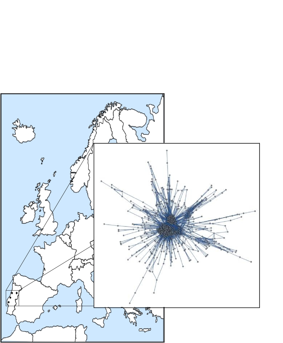
In this paper we analyze a large data set of Eduroam networks at Portuguese Universities (see Fig. 1), with the aim of addressing the problem of human motion at the smallest scales, i.e. within one or a few buildings. Our study follows from previous work[9, 10, 11]. The data set comprises one year of collected information with a sample frequency of one second, a time step that enables to assume the data as continuous monitoring of human mobility, and with a higher spatial resolution than mobile phone calls data sets which enables the motion of human dynamics at its smallest scale. We will show that the statistical features of human mobility at the smallest scales is much closer to the random-walk model than the results obtained for studies at larger scales. Still, the corresponding exponents we find in this study indicate a super-diffusive regime which we address in the end for discussing possible ways of using such statistical information to optimize Eduroam networks when establishing the location of the access points.
The complex network framework has been applied frequently to address social and environmental problems[14, 15, 16, 17, 18]. For recent reviews see [12, 13]. While using the same framework, we introduce here a novel procedure for extracting the network on which persons move at small scales (university buildings), directly from empirical data.
We start in Sec. 2 describing the data sets and in Sec. 3 we introduce tools to properly extract the network of access points. As we will see, the procedure for extracting such network is not trivial since the weight of each connection between two access points is not a straightforward euclidean distance due to the physical constraints (stairs, walls, etc) that condition the movement of persons. In Sec. 4 a detailed description of our finding is presented, enhancing the near-diffusive regime found for human mobility at small scales. Further discussions on how to apply our findings for wireless network optimization as well as the main conclusions are given in Sec. 5.
2 The Eduroam data sets
The data set comprehends a Eduroam RADIUS log file from the University of Minho (Portugal) infrastructure, including the full year of 2011. The file contains a total of data records. From those, refer to “start-events” and refer to “stop-events”. For the present analysis, only records representing stop-events have been used, as they include the disassociation time-stamp and session time from where the start events can be computed. A few amount of these records () have been filtered, since they are incomplete or do not represent unique Access Points or unique Stations. After filtering, records remain for processing and analysis.
Using all these records we will, in the next section, construct the weighted network composed by a number of Access Points (APs), that varies in time. We constructed the AP network considering all APs detected during each full month of 2011. The minimum number of APs was observed in August, namely APs.
For extracting the AP network, we convert the Eduroam database into an output file with three single fields for each record, namely:
-
•
The user , or alternatively the device one user is using when connected to the net. We will address the associated properties of users with lower-case letters.
-
•
The Access Point (AP) . Other properties of APs will also be addressed with capital letters.
-
•
Time in units of the time step second, which is typically the size of the smallest time lag between successive records.
3 The underlying network and its evolution
The global network we aim to construct will be extracted from two complementary networks included in our database.
One part comprehends the network of APs, a network composed solely by the APs, connected among them through weighted links with a weight inversely proportional to their topological distance , that will be properly defined below.
The other part is the network of users, a network composed solely by the links between each connected user and the corresponding AP. The collection of these connections results in a completely disconnected set of APs each one with a number of users exclusively linked to them.
Notice that, the time one user is connected to one AP is quite larger than the unit time-step (1 second). Therefore, by taking snapshots of the entire network at each increment second, the amount of data to analyze increases enormously, compared with the amount of data collected originally. To overcome this shortcoming, the network of users is defined only by the linked-list mapping, at each time step, each connected user to its corresponding AP .
3.1 Access Point fitness and session times
Counting the total number of connected users at one given time step yields the fitness of a particular AP . See Fig. 2a for a typical example on how varies over a few days.
At each time-step , at AP equals the total number of associations occurred at minus the total number of disassociations, occurred within the full time span from the beginning of the observation period up to time . Through time, the fitness illustrated in Fig. 2a shows a daily quasi-periodic pattern, which indicates a maximum time interval of one day for the sessions of connected users. Therefore, to avoid isolated associations we assume that each one cannot last more that hours. Similar assumption can be taken for disassociations. Notice also that the initial value for all is considered to be zero, though it may correspond to same base value of connected devices that varies from AP to AP.
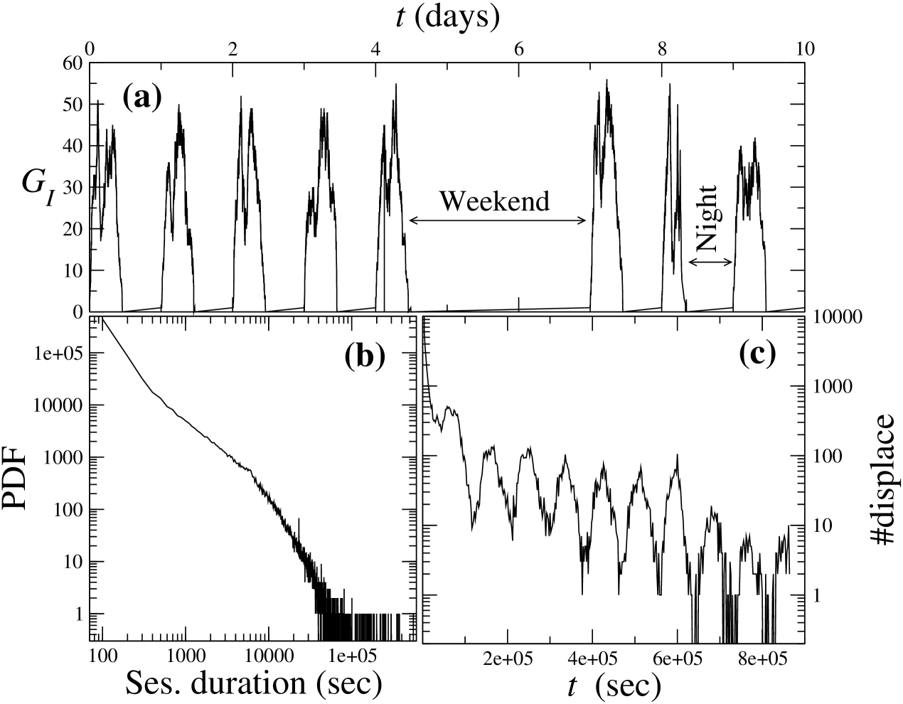
From Fig. 2b one can conclude that the large majority of sessions is shorter than one day, with less than of sessions longer than hours. Therefore, filtering sessions longer than 24 hours has no significant impact on the following analysis and results. Also from Fig. 2c, showing the duration of displacements, one observes a daily pattern. Here, an approximate fit of the distribution of session times is with and (not shown).
Displacements between APs, defined as the disassociation from one AP and subsequent association with AP , exhibit a periodic behavior as illustrated by the distribution of the corresponding time spans (see Fig. 2c). However, the majority of the displacements have a short duration, representing fast displacements among nearby APs.

3.2 Fluxes between Access Points and their topological distance
The network of APs is a weighted network and its adjacency matrix is defined by the elements , where is the distance between APs and . Typically we do not have the location of the APs and we do not know exactly the full number of constraints that condition the displacement of a person from the coverage area of one AP to that of the next one. Therefore we introduce here a definition for the topological distance between APs in such networks.
To that end we need the average fitness at each AP and the flux of users that go from AP to AP , without passing in any intermediate AP. We notice that seasonal fluctuations have been observed while using the network, with the largest variations over the summer (vacations) period (see Fig. 4 below). Therefore, the average fitness at each AP has been calculated for a time window of month and repeated for every month during the entire year. A similar approach has been used for the calculation of the average flux, which yields one AP network for each month.
For computing the flux from to , one reads the output file counting the number of users that associate to AP after disassociating from AP , within a time window day. The instantaneous flux between and is then defined as
| (1) |
From the instantaneous flux the average flux is easily computed as
| (2) |
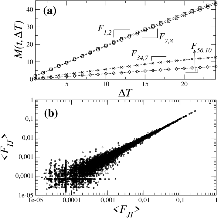
As shown in Fig. 3a, for four different pairs of APs, the average flux is approximately constant within time windows up to one day. Therefore we consider the average flux within hours as an estimate of the flux between each pair of APs to reduce the computation time. For a fixed , the average flux depends on : computing Eq. (2) in different days or weeks yields different results. Still, preliminary results (not shown) indicate that for several pairs of APs the variation of is not very large. Henceforth, we make two assumptions: (i) the fluxes do not vary significantly within one month and (ii) they are well represented through the computation of Eq. (2) for days.
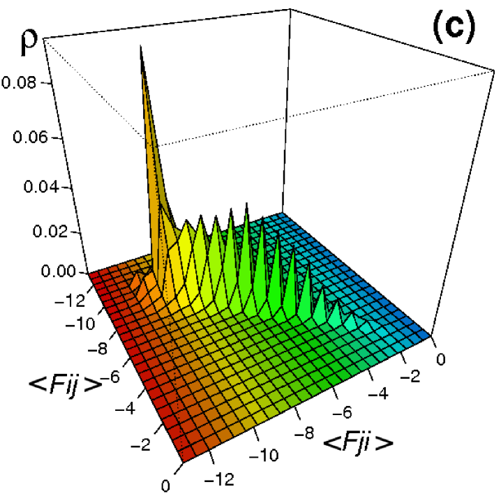
Moreover, as shown in Fig. 3b the fluxes are typically symmetric, i.e. . From these quantities and one finally defines the weight of the connection between AP and as follows:
| (3) |
Here is average over one month.
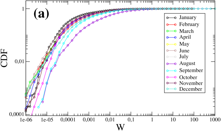
Figure 4a shows the weight distribution (cumulative density functions) for each month in the data set. The weight average – over all AP connections – varies from month to month as well as the corresponding deviations
| (4) |
from a reference month, chosen to be January. Figure 4b shows the evolution through one year of both the average (diamonds) and the deviation (squares) from the average . While some significant variations are observed during the summer vacations, the normalized deviations are constant. This result also highlight the temporal evolution on the usage of the network, with more and more users accessing the network and also more APs being deployed to improve the network capacity.
4 Mobility patterns at small scales
To study the mobility within the universities we do as follows. First, we make use of the inverse weight of the connections between adjacent APs to define a topological distance. Since the weight measures the normalized flux between two adjacent APs, say and , its inverse value can be taken as a good estimate of the topological distance between those APs, which of course defines a symmetric matrix (). Then, having defined the matrix of topological distances between APs, we symbolize the position of one person at time throughout its trajectory as with reference to an initial position, labeled AP . In other words, if person at time is connected to AP , its position is .
Second, having the trajectory followed by one person defined by the successive values of APs, , and also the corresponding distances to the initial AP , we are able to compute the average distance to the initial position as a function of time. Indeed, keeping track of the distance from the initial position, and averaging over all trajectories in the data sets yields the average distance from the initial position:
| (5) |
with labeling one of the trajectories observed at each time and where marks the initial time when the trajectory is started and we chose second.
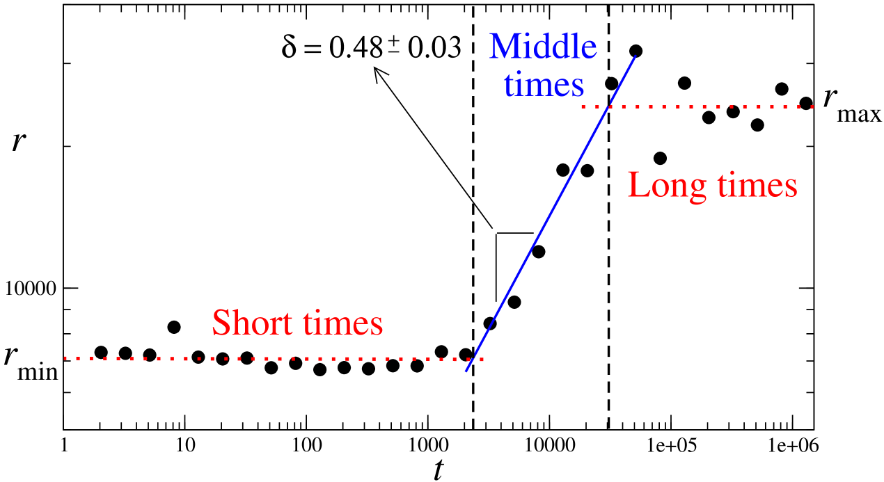
Figure 5 shows the displacement as a function of time averaged over all observed in year 2011. While for short and long times the displacement tends to remain approximately constant at and respectively, for middle times there is a clear scaling with . Short times are shorter than minutes: sessions are too short for observing any significant motion from one AP to the next one. Long times are typically longer than hours, which comprehends the typicall working day of researchers and students in the Eduroam network.
In the study by Gonzalez and co-workers[4], instead of the average distance a radius of gyration was used. The radius of gyration is defined as the linear size occupied by each trajectory up to time and is computed as
| (6) |
where is the “center of mass” of trajectory at time :
| (7) |
The reason why we chose to use the average displacement instead of the radius of gyration lays in the fact that the former is less sensitive to the transition from short times to middle times. For short times the radius of gyration is constant and significantly larger than the average distance. When the trajectory starts to leave the original AP the center of mass of the trajectory increases which leads to a decrease of the radius of gyration. Finally, when the center of mass stabilizes one observes the similar behavior between our average distance and the radius of gyration introduced previously by Gonzalez et al[4]. For long times the radius of gyration stationarizes also approximately at the same value as the average distance.
Having obtained the value of for the average distance one can now proceed to access dynamical features of these human trajectories at small scales.
In general, the exponent characterizes how people “diffuse” in space. For one has the normal Brownian diffusion, which can be describe by a person moving continuously in a random direction in small jumps. If this walker moves slower, with longer waiting times then . On the contrary, if the walker is able to perform large jumps while randomly walking, then . Typically, characterizes the so-called normal diffusion, while and indicate anomalous regimes, sub-diffusive and super-diffusive respectively. For a short review in this topic see Ref. [8].
Based in this knowledge one observes that the exponent is the same as the one for Brownian motion, within numerical error, differently from the exponent found in human mobility studies at larger scales[4]. Indeed in the study by Gonzalez the authors found for mobility within U.S.A. an exponent for the distribution of radius of gyration
| (8) |
Since it is known from scaling analysis that , one finds for the large spatial scales covered in [4]. This value is quite above the value found for the mobility within universities.
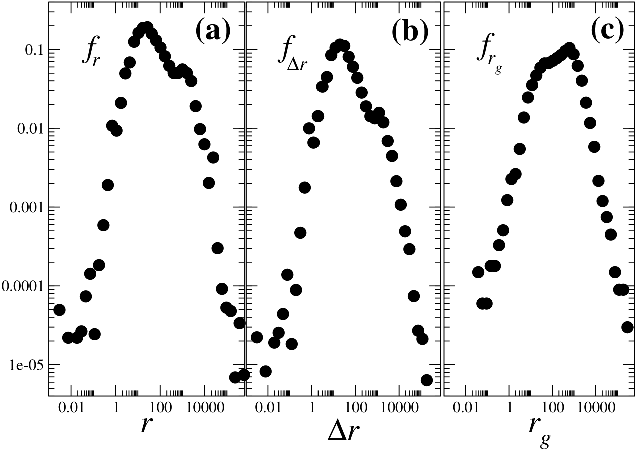
Moreover, the functional form of the distributions given in Eq. (8) is quite different from the one observed in our study. In particular, the power-law tail is for our small spatial scales not observed. Figure 6 shows the distribution together with the distribution for the radius of gyration and also the distribution of the displacement increments . In all cases the distribution shows no power-law tendency. In particular it is characterized by a typical value for , and , resembling therefore much of the Brownian behavior occurring in normal diffusion.
5 Discussion and conclusions
The central finding in this paper is the -value found for human motion at the smallest scale (streets and buildings). This value is close to the one for normal diffusion regime, much lower than the value found in [4] for middle and large scales, cities and countries respectively. What does this mean?
At large scales such as countries it is known that people make large “jumps” with a significant frequency. This is reflected in a large value, considerably above one. As one decreases to smaller scales this large jumps turn to occur more rarely. At the most extreme case, one can think in a set of people moving on a continuous surface not larger than a few hundred meters wide. In this situation the average displacement exponent should be . Within a building however there are physical constraints, such as stairs and walls, that do not promote a normal diffusion of persons. Some deviation from the Brownian exponent would be expected. Still, our procedure for extracting the topological distance between pairs of APs seems to properly account for such spatial constraints in human motion at small scales.
Of course that in our case the position are determined by the locations of the AP. If one changes their location the AP network would be different and, for the same human dynamics, the exponent would be also different. A set of locations corresponding to an exponent is conjectured to be the optimal set of locations, i.e. the one that better suits the flux of persons throughout the building.
Therefore, with the approach we introduce in this paper, one is able to construct a weighted network of APs and evaluate how well it suits the mobility of persons where the APs are placed.
As recently proposed[19], since the Eduroam data base covers the whole of Europe, a possible next step would be to consider the joint data base of several European universities. By properly matching the mask IDs and similar quantities at different universities, one would be able to keep track of individuals throughout Europe and apply the framework described above to data sets comprising larger and larger areas. Since the mobility of faculties and students is becoming higher due to European programs such as Erasmus, one should expect sufficient statistics in the Eduroam databases at several spatial scales. Consequently, one should be able to observe the transition from Brownian to non-Brownian motion, postulated in this paper.
In particular, for the entire region of Asia, eduroam is deployed with top-level RADIUS servers beeing operated by AARNet (Australia) and by the University of Hong Kong. Since this is the broadest region having Eduroam operating, covering the full area from New Zealand to Japan and from South Korea to India, it is of particular interest for assessing the full set of scales where human motion takes place.
Two further points that would be interesting to explore in these data sets are, first, the time evolution of the network of AP, here taken as a static network, and, second, the multifractality of human dynamics at small scales, i.e. to study the dependence of exponent on the order of the moments of the displacement : . These and other points will be addressed elsewhere.
Acknowledgments
The authors thank partial support by Fundação para a Ciência e a Tecnologia under the R&D project PTDC/EIA-EIA/113933/2009. PGL also thanks support from PEst-OE/FIS/UI0618/2011.
References
- [1] L. Guo, X. Cai, Emergence of Community Structure in the Adaptive Social Networks, Commun. Comput. Phys., 8 (2010), 835-844.
- [2] R. Toral, C.J. Tessone, Finite Size Effects in the Dynamics of Opinion Formation, Commun. Comput. Phys., 2 (2007), 177-195.
- [3] J. Ke , T. Gong , W.S. Wang, Language Change and Social Networks, Commun. Comput. Phys., 3 (2008), 935-949.
- [4] M.C. González, C.A. Hidalgo and A.-L. Barabási, Understanding individual human mobility patterns, Nature, 453 (2008), 779-782.
- [5] D. Brockmann, L. Hufnagel and T. Geisel, The scaling laws of human travel, Nature, 439 (2006), 462-465.
- [6] R. Ahas, A. Aasa, Ü. Mark, T. Pae, A. Kull, Seasonal tourism spaces in Estonia: case study with mobile positioning data, Tourism Manag., 28 (2006) 898-910.
- [7] R. Ahas, A. Aasa, S. Silm, R. Aunap, H. Kalle, Ü. Mark, Mobile Positioning in Space – Time Behaviour Studies: Social Positioning Method Experiments in Estonia, Cart. Geog. Inf. Sci., 34 (2007) 259-273.
- [8] M.F. Shlesinger, J. Klafter and G. Zumofen, Above, below and beyond Brownian motion, Am. J. Phys., 67 (1999) 1253-1259.
- [9] A. Moreira, M.Y. Santos, Enhancing a user context by real-time clustering mobile trajectories, Proceedings of the International Conference on Information Technology: coding and computing - ITCC 2005, April 4-8 , Las Vegas, NV, USA, 2005.
- [10] A. Moreira, M.Y. Santos, From GPS tracks to context - Inference of high-level context information through spatial clustering, Proceedings of the II International Conference & Exhibition on Geographic Information - GIS Planet 2005, May 30 - June 2, Estoril, Portugal, 2005.
- [11] F. Meneses, A. Moreira, Using GSM CellID Positioning for Place Discovering, Proceedings of the Locare’06 – First Workshop on Location Based Services for Health Care, Innsbruck, Austria, November 28, 2006.
- [12] S. Boccaletti, V. Latora, Y. Moreno, M. Chavez and D.-U. Hwang, Complex networks: Structures and dynamics, Phys. Rep., 424 (2006), 175-308.
- [13] S.N. Dorogovtsev, A.V. Goltsev, J.F.F. Mendes: Critical phenomena in complex networks, Rev. Mod. Phys., 80 (2008), 1275-1354.
- [14] P.G. Lind, M.C. González and H.J. Herrmann: Cycles and clustering in bipartite networks, Phys. Rev. E, 72 (2005), 056127.
- [15] M.C. González, P.G. Lind and H.J. Herrmann, A system of mobile agents to model social networks, Phys. Rev. Lett., 96 (2006), 088702.
- [16] M.C. González, P.G. Lind and H.J. Herrmann, Networks based on collisions among mobile agents, Physica D, 224 (2006), 137-148.
- [17] P.G. Lind and H.J. Herrmann, New approaches to model and study social networks, New J. Phys., 9 (2007), 228.
- [18] P.G. Lind, J.S. Andrade Jr., L.R. da Silva, H.J. Herrmann: Model of mobile agents for sexual interactions networks, Europhys. Lett., 78 (2007), 68005.
- [19] F. Raischel, A. Moreira, P.G. Lind, From human mobility to renewable energies, Eur. J. Phys. Spec. Top. to appear (2014).