hunchback promoters can readout morphogenetic positional information in less than a minute
Abstract
The first cell fate decisions in the developing fly embryo are made very rapidly : hunchback genes decide in a few minutes whether a given nucleus follows the anterior or the posterior developmental blueprint by reading out the positional information encoded in the Bicoid morphogen. This developmental system constitutes a prototypical instance of the broad spectrum of regulatory decision processes that combine speed and accuracy. Traditional arguments based on fixed-time sampling of Bicoid concentration indicate that an accurate readout is not possible within the short times observed experimentally. This raises the general issue of how speed-accuracy tradeoffs are achieved. Here, we compare fixed-time sampling strategies to decisions made on-the-fly, which are based on updating and comparing the likelihoods of being at an anterior or a posterior location. We found that these more efficient schemes can complete reliable cell fate decisions even within the very short embryological timescales. We discuss the influence of promoter architectures on the mean decision time and decision error rate and present concrete promoter architectures that allow for the fast readout of the morphogen. Lastly, we formulate explicit predictions for new experiments involving Bicoid mutants.
Keywords Regulation Biological decisions Speed-accuracy Morphogenesis Drosophila Cell fate
0 Introduction
From development to chemotaxis and immune response, living organisms make precise decisions based on limited information cues and intrinsically noisy molecular processes, such as the readout of ligand concentrations by specialized genes or receptors [1, 2, 3, 4, 5]. Selective pressure in biological decision-making is often strong, for reasons that range from predator evasion to growth maximisation or fast immune clearance. In development, early embryogenesis of insects and amphibians unfolds outside of the mother, which arguably imposes selective pressure for speed to limit the risks of predation and infection by parasitoids [6]. In Drosophila embryos, the first 13 cycles of DNA replication and mitosis occur without cytokinesis, resulting in a multinucleated syncytium containing about 6,000 nuclei [7]. Speed is witnessed both by the rapid and synchronous cleavage divisions observed over the cycles, and the successive fast decisions on the choice of differentiation blueprints, which are made in less than 3 minutes [8].
In the early fly embryo, the map of the future body structures is set by the segmentation gene hierarchy [9, 1, 10]. The definition of the positional map starts by the emergence of two (anterior and posterior) regions of distinct hunchback (hb) expression, which are driven by the readout of the maternal Bicoid (Bcd) morphogen gradient (Fig. 1 A). hunchback spatial profiles are sharp and the variance in hunchback expression of nuclei at similar positions along the AP axis is small [11, 8]. Taken together, these observations imply that the short-time readout is accurate and has a low error. Accuracy ensures spatial resolution and the correct positioning of future organs and body structures, while low errors ensure reproducibility and homogeneity among spatially close nuclei. The amount of positional information available at the transcriptional locus is close to the minimal amount necessary to achieve the required precision [12, 13, 14, 15]. Furthermore, part of the morphogenetic information is not accessible for reading by downstream mechanisms [16], as information is channeled and lost through subsequent cascades of gene activity. In spite of that, by the end of nuclear cycle 14 the positional information encoded in the gap gene readouts is sufficient to correctly predict the position of each nucleus within of the egg length [15]. Adding to the time constraints, mitosis resets the binding of transcription factors (TF) during the phase of synchronous divisions, suggesting that the decision about the nuclei’s position is made by using information accessible within one nuclear cycle. Experiments additionally show that during the nuclear cycles 10-13 the positional information encoded by the Bicoid gradient is read out by hunchback promoters precisely and within 3 minutes.
Effective speed-accuracy tradeoffs are not specific to developmental processes, but are shared by a large number of sensing processes. This generality has triggered interest in quantitative limits and mechanisms for accuracy. Berg and Purcell derived the seminal tradeoff between integration time and readout accuracy for a receptor evaluating the concentration of a ligand [17] based on its average binding occupancy. Later studies showed that this limit takes more complex forms when rebinding events of detached ligands [18, 19] or spatial gradients [20] are accounted for. The accuracy of the averaging method in [17] can be improved by computing the maximum likelihood estimate of the time series of receptor occupancy for a given model [21, 22]. However, none of these approaches can result in a precise anterior-posterior (AP) decision for the hunchback promoter in the short time of the early nuclear cycles, which has led to the conclusion that there is not enough time to apply the fixed-time Berg-Purcell strategy with the desired accuracy [23]. Additional mechanisms to increase precision (including internuclear diffusion) do yield a speed-up [24, 25], yet they are not sufficient to meet the 3 minutes challenge. The issue of the embryological speed-accuracy tradeoff remains open.
The approaches described above are fixed-time strategies of decision-making, i.e., they assume that decisions are made at a pre-defined deterministic time that is set long enough to achieve the desired level of error and accuracy. As a matter of fact, fixing the decision time is not optimal because the amount of available information depends on the specific statistical realization of the noisy signal that is being sensed. The time of decision should vary accordingly and therefore depend on the realization. This intuition was formalized by A. Wald by his Sequential Probability Ratio Test (SPRT) [26]. SPRT achieves optimality in the sense that it ensures the fastest decision strategy for a given level of expected error. The adaption of the method to biological sensing posits that the cell discriminates between two hypothetical concentrations by accumulating information through binding events, and by computing on the fly the ratio of the likelihoods (or appropriate proxies) for the two concentrations to be discriminated [27]. When the ratio “strongly” favors one of the two hypotheses, a decision is triggered. The strength of the evidence required for decision-making depends on the desired level of error. For a given level of precision, the average decision time can be substantially shorter than for traditional averaging algorithms [27]. SPRT has also been proposed as an efficient model of decision-making in the fields of social interactions and neuroscience [28, 29] and its connections with non-equilibrium thermodynamics are discussed in [30].
Wald’s approach is particularly appealing for biological concentration readouts since many of them, including the anterior-posterior decision faced by the hunchback promoter, appear to be binary decisions. Our first goal here is to specifically consider the paradigmatic example of the hunchback promoter and elucidate the degree of speed-up that can be achieved by decisions on the fly. Second, we investigate specific implementations of the decision strategy in the form of possible hunchback promoter architectures. We specifically ask how cooperative TF binding affects the sensing limits. Our results have implications beyond fly development and are generally relevant to regulatory processes. We identify promoter architectures that, by approximating Wald’s strategy, do satisfy several key experimental constraints and reach the experimentally observed level of accuracy of hunchback expression within the (apparently) very stringent time limits of the early nuclear cycles.
1 Methodological setup
1.1 The decision process of the anterior vs posterior hunchback expression
The problem faced by nuclei in their decision of anterior vs posterior developmental fate is sketched in Fig. 1 a. We limit our investigation of promoter architectures to the six experimentally identified Bicoid binding sites (Fig. 1 b). We do not consider the known Hunchback binding sites because before nuclear cycle there is little time to produce sufficient concentrations of zygotic proteins for a significant feedback effect and the measured maternal hunchback profile has not been shown to alter anterior-posterior decision-making. Following the observation that Bcd readout is the leading factor in nuclei fate determination [31], we also neglect the role of other maternal gradients, e.g. Caudal, Zelda or Capicua [32, 33, 34, 8], since the readout of these morphogens can only contribute additional information and decrease the decision time. We focus on the proximal promoter since no active enhancers have been identified for the hunchback locus in nuclear cycles 11-13 [35]. Our results can be generalized to enhancers, the addition of which only further improves the speed-accuracy efficacy. Since our goal is to show that accurate decisions can be made rapidly, we focus on the worst case decision-making scenario: the positional information [36] is gathered through a readout of the Bicoid concentration only, and the decision is assumed to be made independently in each nucleus. Having additional information available and/or coupling among nuclei can only strengthen our conclusion.
The profile of the average concentration of the maternal morphogen Bicoid is well represented by an exponential function that decreases from the anterior toward the posterior of the embryo : , where is the position along the anterior-posterior axis measured in terms of percentage egg-length (EL), and is the position of half maximum hb expression corresponding to Bcd concentration. The decay length corresponds to EL [23]. Nuclei convert the graded Bicoid gradient into a sharp border of hunchback expression (Fig. 1 a), with high and low expressions of the hunchback promoter at the left and the right of the border respectively [37, 38, 39, 12, 1, 13, 14, 40, 34, 8]. We define the border region of width symmetrically around by the dashed lines in Fig. 1 a. is related to the positional resolution [24, 34] of the anterior-posterior decision: it is the minimal distance measured in percentages of egg-length between two nuclei’s positions, at which the nuclei can distinguish the Bcd concentrations. Although this value is not known exactly, a lower bound is estimated as EL [23], which corresponds to the width of one nucleus.
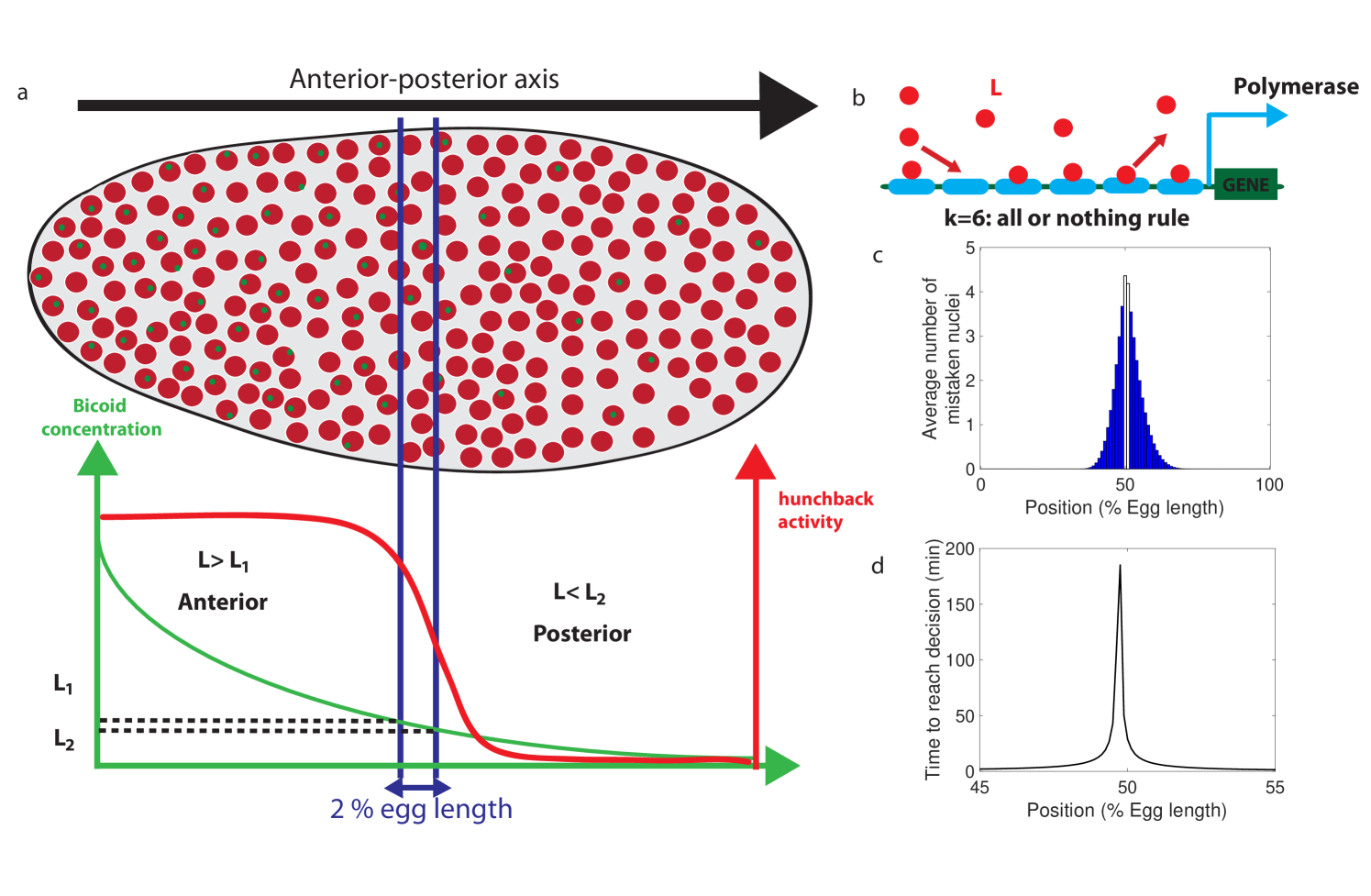
We denote the Bcd concentration at the anterior (respectively posterior) boundary of the border region by (respectively ) (see Fig. 1 a). At each position , nuclei compare the probability that the local concentration is greater than (anterior) or smaller than (posterior). By using current best estimates of the parameters (see Appendix A), a classic fixed-time-decision integration process and an integration time of seconds (the duration of the interphase in nuclear cycle [34]), we compute in Fig. 1 c the probability of error per nucleus for each position in the embryo (see Appendix B for details). As expected, errors occur overwhelmingly in the vicinity of the border region, where the decision is the hardest (Fig. 1 c). For nuclei located within the border region, both anterior and posterior decisions are correct since the nuclei lie close to both regions. It follows that, although the error rate can formally be computed in this region, the errors do not describe positional resolution mistakes and do not contribute to the total error (white zone in Fig. 1 c).
In view of Fig. 1 c and to simplify further analysis we shall focus on the boundaries of the border region : each nucleus discriminates between hypothesis – the Bcd concentration is , and hypothesis – the Bcd concentration is . To achieve a positional resolution of EL, nuclei need to be able to discriminate between differences in Bcd concentrations on the order of : . In addition to the variation in Bcd concentration estimates that are due to biological precision, concentration estimated using many trials follows a statistical distribution. The central limit theorem suggests that this distribution is approximately Gaussian. This assumption means that the probability that the Bcd concentration estimate deviates from the actual concentration by more than the prescribed positional resolution is (see Section 2.1.1 for variations on the value and arguments on the error rate). In Fig. 1 d we show that the time required under a fixed-time-decision strategy for a promoter with six binding sites to estimate the Bcd concentration within the Gaussian error rate [23] close to the boundary is much longer than seconds, minutes ( see Appendix B for details of the calculation). The activation rule for the promoter architecture in the figure is that all binding sites need to be bound for transcription initiation.
1.2 Identifying fast decision promoter architectures
1.2.1 The promoter model
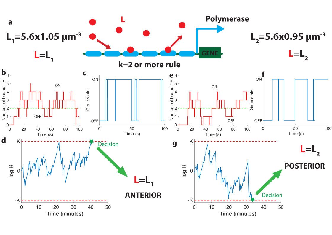
We model the hb promoter as six Bcd binding sites [41, 42, 43, 44] that determine the activity of the gene (Fig. 2 a). Bcd molecules bind to and unbind from each of the sites with rates and , which are allowed to be different for each site. For simplicity, the gene can only take two states : either it is silenced (OFF) and mRNA is not produced, or the gene is activated (ON) and mRNA is produced at full speed. While models that involve different levels of polymerase loading are biologically relevant and interesting, the simplified model allows us to gain more intuition and follows the worst-case scenario logic that we discussed in section 1.1. The same remark applies for the wide variety of promoter architectures considered in previous works [45, 34]. In particular, we assume that only the number of sites that are bound matters for gene activation (and not the specific identity of the sites). Such architectures are again a subset of the range of architectures considered in [45, 34].
The dynamics of our model is a Markov chain with seven states with probability corresponding to the number of sites occupied: from all sites unoccupied (probability ) to all six sites bound by Bcd molecules (probability ). The minimum number of bound Bicoid sites required to activate the gene divides this chain into the two disjoint and complementary subsets of active states (, for which the gene is activated) and inactive states (, for which the gene is silenced) as illustrated in Fig. 2 b and d.
As Bicoid ligands bind and unbind the promoter (Fig. 2 b), the gene is successively activated and silenced (Fig. 2 c). This binding/unbinding dynamics results in a series of OFF and ON activation times that constitute all the information about the Bcd concentration available to downstream processes to make a decision. We note that the idea of translating the statistics of binding-unbinding times into a decision remains the same as in the Berg-Purcell approach, where only the activation times are translated into a decision (and not the deactivation times). The promoter architecture determines the relationship between Bcd concentration and the statistics of the ON-OFF activation time series, which makes it a key feature of the positional information decision process. Following Ref. [27], we model the decision process as a Sequential Probability Ratio Test (SPRT) based on the time series of gene activation. At each point in time, SPRT computes the likelihood of the observed time series under both hypotheses and and takes their ratio : . The logarithm of undergoes stochastic changes until it reaches one of the two decision threshold boundaries or (symmetric boundaries are used here for simplicity) (Fig. 2 d). The decision threshold boundaries are set by the error rate for making the wrong decision between the hypothetical concentrations : (see [27] and Appendix C.5). The choice of or depends on the level of reproducibility desired for the decision process. We set , corresponding to the widely used error rate of being more than one standard deviation away from the mean of the estimate for the concentration assumed to be unbiased in a Gaussian model (see Section 1.1 above). The statistics of the fluctuations in likelihood space are controlled by the values of the Bcd concentrations: when Bcd concentration is low, small numbers of Bicoid ligands bind to the promoter (Fig. 2 e) and the hb gene spends little time in the active expression state (Fig. 2 f), which leads to a negative drift in the process and favors the lower one of the two possible concentrations (Fig. 2 g).
1.2.2 Mean decision time : connecting drift-diffusion and Wald’s approaches
In this section, we develop new methods to determine the statistics of gene switches between the OFF and ON expression states. Namely, by relating Wald’s approach [26] with drift-diffusion, we establish the equality between the drift and diffusion coefficients in decision making space for difficult decision problems, i.e. when the discrimination is hard, we elucidate the reason underlying the equality. That allows us to effectively determine long-term properties of the likelihood log-ratio and compute mean decision times for complex architectures.
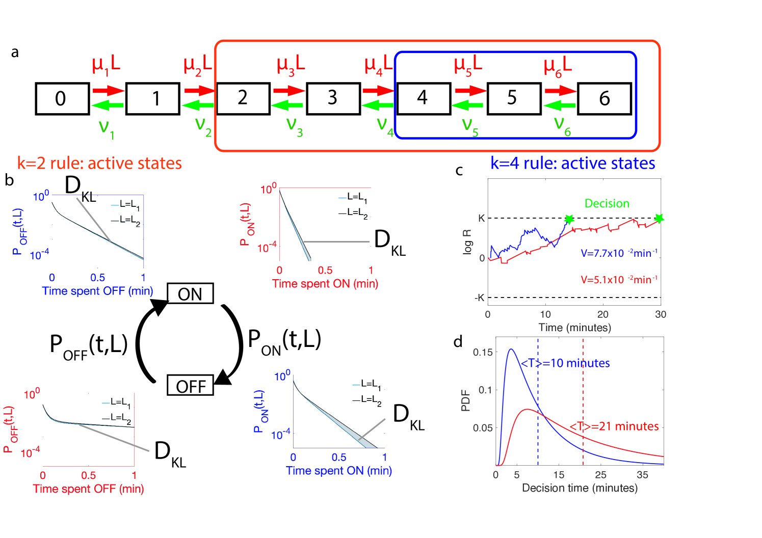
A gene architecture consists of binding sites and is represented by Markov states corresponding to the number of bound TF, and the rates at which they bind or unbind (Fig. 3 a). For a given architecture, the dynamics of binding/unbinding events and the rules for activation define the two probability distributions and for the duration of the OFF and ON times, respectively (Fig. 3b). The two series are denoted and , where and are the number of switching events in time from OFF to ON and vice versa. For those cases where the two concentrations and are close and the discrimination problem is difficult (which is the case of the Drosophila embryo), an accurate decision requires sampling over many activation and deactivation events to achieve discrimination. The logarithm of the ratio can then be approximated by a drift–diffusion equation: , where is the constant drift, i.e. the bias in favor of one of the two hypotheses, is the diffusion constant and a standard Gaussian white noise with zero mean and delta-correlated in time [26, 27]. The decision time for the case of symmetric boundaries , is given by the mean first-passage time for this biased random walk in the log-likelihood space [46, 27]:
| (1) |
Note that in this approximation all the details of the promoter architecture are subsumed into the specific forms of the drift and the diffusion .
Drift. We assume for simplicity that the time series of OFF and ON times are independent variables (when this assumption is relaxed, see Appendix G). This assumption is in particular always true when gene activation only depends on the number of bound Bicoid molecules. Under these assumptions we can apply Wald’s equality [47, 48] to the log-likelihood ratio, . Wald considered the sum of a random number of independent and identically distributed (i.i.d.) variables. The equality that he derived states that if is independent of the outcome of variables with higher indices (i.e. is a stopping time), then the average of the sum is the product .
Wald’s equality applies to our likelihood sum ( of the likelihoods, where is the number of ON and OFF times before a given (large) time ). We conclude the drift of the log-likelihood ratio, , is inversely proportional to , where is the mean of the distribution of ON times and is the mean of the distribution of OFF times . The term determines the average speed at which the system completes an activation/deactivation cycle, while the average describes how much deterministic bias the system acquires on average per activation/deactivation cycle. The latter can be re-expressed in terms of the Kullback-Leibler divergence between the distributions of the OFF and ON times calculated for the actual concentration and each one of the two hypotheses, and :
| (2) | ||||
Eq. 2 quantifies the intuition that the drift favors the hypothetical concentration with the time distribution which is the closest to that of the real concentration (Fig. 3 b).
Diffusivity : Why it is more involved to calculate and how we circumvent it. While the drift has the closed simple form in Eq. 2, the diffusion term is not immediately expressed as an integral. The qualitative reason is as follows. Computing the likelihood of the two hypotheses requires computing a sum where the addends are stochastic (ratios of likelihoods) and the number of terms is also stochastic (the number of switching events). These two random variables are correlated: if the number of switching events is large, then the times are short and the likelihood is probably higher for large concentrations. While the drift is linear in the above sum (so that the average of the sum can be treated as shown above), the diffusivity depends on the square of the sum. The diffusivity involves then the correlation of times and ratios [49], which is harder to obtain as it depends a priori on the details of the binding site model (see Appendices C.5 and C.7 for details).
We circumvent the calculation of the diffusivity by noting that the same methods used to derive Eq. (1) also yield the probability of first absorption at one of the two boundaries, say (see Appendix C.5) :
| (3) |
By imposing , we obtain and the comparison with the expression of leads to the equality .
The above equality is expected to hold for difficult decisions only. Indeed, drift-diffusion is based on the continuity of the log-likelihood process and Wald’s arguments assume the absence of substantial jumps in the log-likelihood over a cycle. In other words, the two approaches overlap if the hypotheses to be discriminated are close. For very distinct hypotheses (easy discrimination problems) the two approaches may differ from the actual discrete process of decision and among themselves. We expect then that holds only for hypotheses that are close enough, which is verified by explicit examples (see Appendix C.5). The Appendix also verifies by expanding the general expression of and for close hypotheses. The origin of the equality is discussed below.
Using , we can reduce the general formula Eq. (1) to
| (4) |
which is formula in [26] and it is the expression that we shall be using (unless stated otherwise) in the remainder of the paper.
The additional consequence of the equality is that the argument of the hyperbolic tangent in Eq. (1) is . It follows that for any problem where the error , the argument of the hyperbolic tangent is large and the decision time is weakly dependent on deviations to that occur when the two hypotheses differ substantially. A concrete illustration is provided in Appendix C.6.
Single binding site example. As an example of the above equations, we consider the simplest possible architecture with a single binding site (), where the gene activation and de-activation processes are Markovian. In this case the de-activation rate is independent of TF concentration and the activation rate is exponentially distributed . We can explicitly calculate the drift (Eq. 2) and expand it for and , at leading order in . Inserting the resulting expression into Eq. 4, we conclude that
| (5) |
decreases with increasing relative TF concentration difference and gives a very good approximation of the complete formula (see SI Fig 9 a-c with different values of ).
Eqs. 2 and 4 greatly reduce the complexity of evaluating the performance of architectures, especially when the number of binding sites is large. Alternatively, computing the correlation of times and log-likelihoods would be increasingly demanding as the size of the gene architecture transfer matrices increase. As an illustration, Fig. 3 compares the performance of different activation strategies : the -or-more rule (), which requires at least two Bcd binding sites to be occupied for hb promoter activation (Fig. 3a-d in blue), and the -or-more rule () (Fig. 3a-d in red) for fixed binding and unbinding parameters. Fig. 3c shows that stronger drifts lead to faster decisions. The full decision time probability distribution is computed from the explicit formula for its Laplace transform [27] (Fig. 3d). With the rates chosen for Fig. 3, the rule leads to an ON time distribution that varies strongly with the concentration, making it easier to discriminate between similar concentrations: it results in a stronger average drift that leads to a faster decision than (Fig. 3 d).
What is the origin of the equality? The special feature of the SPRT random process is that it pertains to a log-likelihood. This is at the core of the equality that we found above. First, note that the equality is dimensionally correct because log-likelihoods have no physical dimensions so that both and have units of . Second, and more important, log-likelihoods are built by Bayesian updating, which constrains their possible variations. In particular, given the current likelihoods and at time for the two concentrations and and the respective probabilities and of the two hypotheses, it must be true that the expected values after a certain time remain the same if the expectation is taken with respect to the current (see, e.g. [50]). In formulae, this implies that the average variation of the probability over a given time that is
| (6) |
should vanish (see Appendix C.5 for a derivation). Here, is the expected variation of under the assumption that hypothesis is true and is the same quantity but under the assumption that hypothesis is true. We notice now that , where is the log-likelihood, and that the drift-diffusion of the log-likelihood implies that , and . By using that and , we finally obtain that
| (7) |
and imposing yields the equality . Note that the above derivation holds only for close hypotheses, otherwise the velocity and the diffusivity under the two hypotheses do not coincide.
1.2.3 Additional embryological constraints on promoter architectures
In addition to the requirements imposed by their performance in the decision process (green dashed line in Fig. 4a), promoter architectures are constrained by experimental observations and properties that limit the space of viable promoter candidates for the fly embryo. A discussion about their possible function and their relation to downstream decoding processes is deferred to the final section.
First, we require that the average probability for a nucleus to be active in the boundary region is equal to , as it is experimentally observed [40] (Fig. 1a). This requirement mainly impacts and constrains the ratio between binding rates and unbinding rates .
Second, there is no experimental evidence for active search mechanisms of Bicoid molecules for its targets. It follows that, even in the best case scenario of a Bcd ligand in the vicinity of the promoter always binding to the target, the binding rate is equal to the diffusion limited arrival rate (Appendix A). As a result, the binding rates are limited by diffusion arrivals and the number of available binding sites: (black dashed line in Fig. 4b), where is the concentration of Bicoid. This sets the timescale for binding events. In Appendix A, we explore the different measured values and estimates of parameters defining the diffusion limit and their influence on the decision time (see Table 1 for all the predictions).
Third, as shown in Fig. 1, the hunchback response is sharp, as quantified by fitting a Hill function to the expression level vs position along the egg length. Specifically, the hunchback expression (in arbitrary units) is well approximated as a function of the Bicoid concentration by the Hill function , where is the Bcd concentration at the half-maximum expression point and is the Hill coefficient (Fig. 1a). Experimentally, the measured Hill coefficient for mRNA expression from the WT hb promoter is [8, 34]. Recent work [34] suggests that these high values might not be achieved by Bicoid binding sites only. Given current parameter estimates and an equilibrium binding model, [34] shows that a Hill coefficient of is not achievable within the duration of an early nuclear cycle ( min). That points at the contribution of other mechanisms to pattern steepness. Given these reasons (and the fact that we limit ourselves only to a model with equilibrium Bcd binding sites only), we shall explore the space of possible equilibrium promoter architectures limiting the steepness of our profiles to Hill coefficients .
1.2.4 Numerical procedure for identifying fast decision-making architectures
Using Eqs. 2 and 4, we explore possible hb promoter architectures and activation rules to find the ones that minimize the time required for an accurate decision, given the constraints listed in Section 1.2.3. We optimize over all possible binding rates ( is the binding rate of the first Bcd ligand and the binding rate of the last Bcd ligand when Bcd ligands are already bound to the promoter), and the unbinding rates ( is the unbinding rate of a single Bcd ligand bound to the promoter and is the unbinding rate of all Bcd ligands when all six Bcd binding sites are occupied). We also explore different activation rules by varying the minimal number of Bcd ligands required for activation in the -or-more activation rule [45, 34]. We use the most recent estimates of biological constants for the hb promoter and Bcd diffusion (see Appendix A) and set the error rate at the border to [12, 15]. Reasons for this choice were given in subsection 1.1 and will be revisited in subsection 2.1.1, where we shall introduce some embryological considerations on the number of nuclei involved in the decision process and determine the error probability accordingly. The optimization procedure that minimized the average decision time for different values of and is implemented using a mixed strategy of multiple random starting points and steepest gradient descent (Fig. 4a).
2 Results
2.1 Logic and properties of the identified fast decision architectures
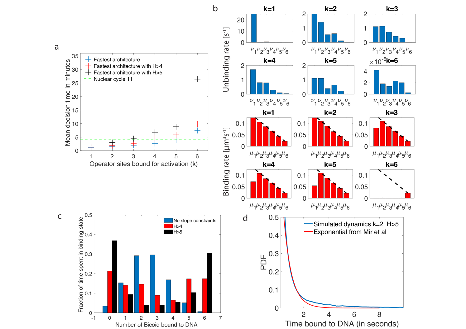
The main conclusion we reach using the methodology presented in section 1 is that there exist promoter architectures that reach the required precision within a few minutes and satisfy all the additional embryological constraints that were discussed previously (Fig. 4a). The fastest promoters (blue crosses in Fig. 4a) reach a decision within the time of nuclear cycle 11 (green line in Fig. 4a) for a wide range of activation rules. Even imposing steep readouts () allows us to identify relatively fast promoters, although imposing the nuclear cycle time limit, pushes the activation rule to smaller . The optimal architectures differ mainly by the distribution of their unbinding rates (Fig. 4b). We shall now discuss their properties, namely the binding times of Bicoid molecules to the DNA binding sites, and the dependence of the promoter activity on various features, such as activation rules and the number of binding sites in detail. Together, these results elucidate the logic underlying the process of fast decision-making.
2.1.1 How many nuclei make a mistake?
The precision of a stochastic readout process is defined by two parameters: the resolution of the readout , and the probability of error, which sets the reproducibility of the readout. In Fig. 4 we have used the statistical Gaussian error level () to obtain our results. However, the error level sets a crucial quantity for a developing organism and it is important to connect it with the embryological process, namely how many nuclei across the embryo will fail to properly decide (whether they are positioned in the anterior or in the posterior part of the embryo). To make this connection, we compute this number for a given average decision time and we integrate the error probability along the AP axis to obtain the error per nucleus . The expected number of nuclei that fail to correctly identify their position is given by , where is the nuclear cycle and we have neglected the loss due to yolk nuclei remaining in the bulk and arresting their divisions after cycle [51]. Assuming a s readout time – the total interphase time of nuclear cycle ([34]) – for the fastest architecture identified above and an error rate of , we find that , that is an essentially fail-proof mechanism. This number can be compared with nuclei in the embryo that make an error in a s read-out in a Berg-Purcell-like fixed time scheme (integrated blue area in Fig. 1c).
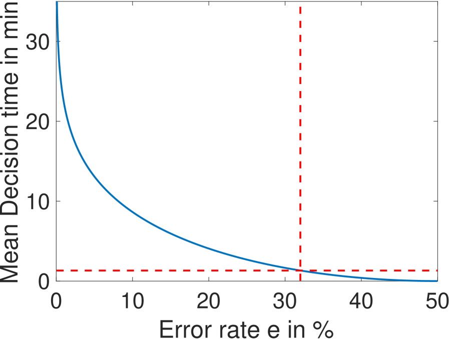
Conversely, for a given architecture, reducing the error level increases drastically the mean first-passage time to decision: the mean time for decision as a function of the error rate for the fastest architecture identified with and is shown in Fig. 7. The decision can be made in about a minute for but requires on average minutes for (Fig. 7). Note that, because the mean first-passage depends simply on the inverse of the drift per cycle (Eq. 4), the relative performance of two architectures is the same for any error rate so that the fastest architectures identified in Fig. 4a are valid for all error levels.
2.1.2 Residence times among the various states
As shown in Ref. [34], high Hill coefficients in the hunchback response are associated with frequent visits of the extreme expression states where available binding sites are either all empty (state ), or all occupied (state ). Fig. 4c provides a concrete illustration by showing the distribution of residence times for the promoter architectures that yield the fastest decision times for and no constraints (blue bars), (red bars) and (black bars). When there are no constraints on the slope of the hunchback response, the most frequently occupied states are close to the ON-OFF transition ( and occupied binding sites in Fig. 4c) to allow for fast back and forth between the active and inactive states of the gene and thereby gather information more rapidly by reducing (see formulae 2 and 4).
We notice that for higher Hill coefficients, the system transits quickly through the central states (in particular states with and occupied Bcd sites, Fig. 4 red and black bars). As expected for high Hill coefficients, such dynamics requires high cooperativity. Cooperativity helps the recruitment of extra transcription factors once one or two of them are already bound and thus speeds up the transitioning through the states with , and occupied binding sites. An even higher level of cooperativity is required to make TF DNA binding more stable when or of them are bound, reducing the OFF rates or (Fig. 4b).
2.1.3 The (short) binding times of Bicoid on DNA
The distribution of times spent bound to DNA of individual Bicoid molecules is shown in Fig. 4d obtained from Monte Carlo simulations using rates from the fastest architecture with and . We find an exponential decay, an average bound time of about s and a median around s. Our median-time-bound prediction is of the same order of magnitude as the observed bound times seen in recent experiments by Mir et al [52], who found short (mean s and median s based on exponential fits), yet quite distinguishable from background, bound times to DNA. These results were considered surprising because it seemed unclear how such short binding events could be consistent with the processing of ON and OFF gene switching events. Our results show that such short binding times may actually be instrumental in achieving the tradeoff between accuracy and speed, and rationalize how longer activation events are still achieved despite the fast binding and unbinding. High cooperativity architectures lead to non-exponential bound times to DNA (Fig. 4d) for which the typical bound time (median) is short but the tail of the distribution includes slower dynamics that can explain longer activation events (the mean is much larger than the median). This result suggests that cells can use the bursty nature of promoter architectures to better discriminate between TF concentrations.
In Ref. [52], the raw distribution comprises both non-specific and specific binding and cannot be directly compared to simulation results. Instead, we use the largest of the two exponents fit for the boundary region [52], which should correspond to specific binding. The agreement between the distributions in Fig. 4d is overall good, and we ascribe discrepancies to the fact that Mir et al. [52] fit two exponential distributions assuming the observed times were the convolution of exponential specific and non-specific binding times. Yet the true specific binding time distribution is likely not exponential, e.g. due to the effect of binding sites having different binding affinities. We show in Supplementary Fig. 13 that the two distributions are very similar and hard to distinguish once they are mixed with the non-specific part of the distribution.
2.1.4 Activation rules
In the parameter range of the early fly embryo, the fastest decision-making architectures share the -or-more () activation rule : the promoter switches rapidly between the ON and OFF expression states and the extra binding sites are used for increasing the size of the target rather than building a more complex signal. Architectures with and activation rules can make decisions in less than seconds and satisfy all the required biological constraints. Generally speaking, our analysis predicts that fast decisions require a small number of Bicoid binding sites (less than three) to be occupied for the gene to be active. The advantage of the or activation rules is that the ON and OFF times are on average longer than for , which makes the downstream processing of the readout easier. We do not find any architecture satisfying all the conditions for the activation rules, although we cannot exclude there could be some architectures outside of the subset that we managed to sample, especially for the activation rules where we did identify some promoter structures that are close to the time constraint.
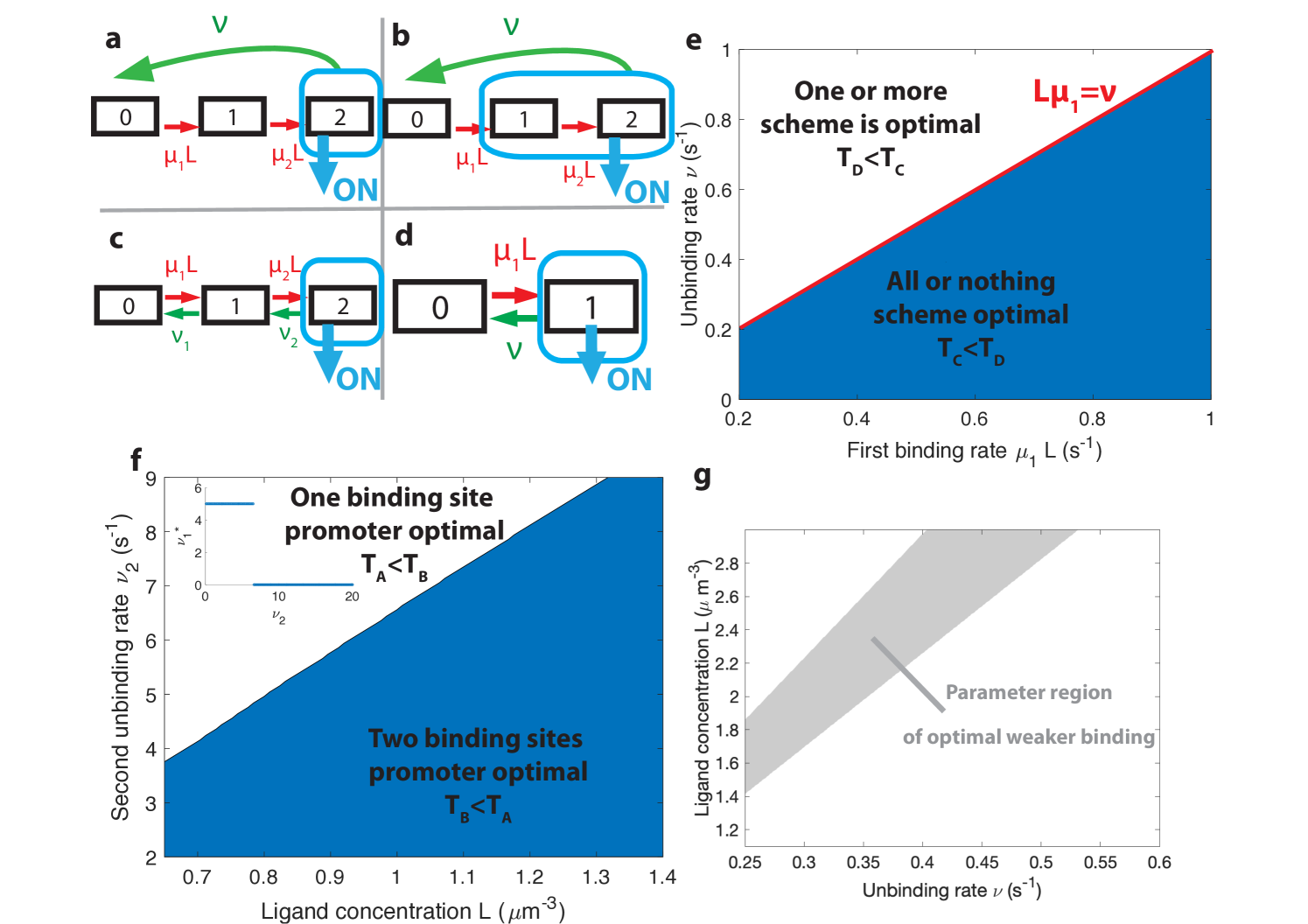
Activation rules with higher can give higher information per cycle for the ON rate, yet they do not seem to lead to faster decisions because of the much longer duration of the cycles. To gain insight on how the tradeoff between fast cycles and information affects the efficiency of activation rules, we consider architectures with only two binding sites, which lend to analytical understanding (Fig. 5 a and b). Both of these considered architectures are out of equilibrium and require energy consumption (as opposed to the two equilibrium architectures of Fig. 5 c and d).
When is -or-more faster than all-or-nothing activation? A first model has the promoter consisting of two binding sites with the all-or-nothing rule (Fig. 5 a). We consider the mathematically simpler, although biologically more demanding, situation where TFs cannot unbind independently from the intermediate states – once one TF binds, all the binding sites need to be occupied before the promoter is freed by the unbinding with rate of the entire complex of TFs. This situation can be formulated in terms of a non-equilibrium cycle model, depicted for two binding sites in Fig. 5 a. The activation time is a convolution of the exponential distributions . In the simple case when the two binding rates are similar (), the OFF times follow a Gamma distribution and the drift and diffusion can be computed analytically (see Appendix D). When the two binding rates are not similar the drift and diffusion must be obtained by numerical integration (see Appendix D).
In the first model described above (Fig. 5 a), deactivation times are independent of the concentration and do not contribute to the information gained per cycle and, as a result, to . To explore the effect of deactivation time statistics on decision times, we consider a cycle model where the gene is activated by the binding of the first TF (the -or-more rule) and deactivation occurs by complete unbinding of the TFs complex (Fig. 5 b). The resulting activation times are exponentially distributed and contribute to drift and diffusion as in the simple two state promoter model (Fig. 5 d). The deactivation times are a convolution of the concentration-dependent second binding and the concentration-independent unbinding of the complex and their probability distribution is . Drift and diffusion can be obtained analytically (Appendix D). The concentration-dependent deactivation times prove informative for reducing the mean decision time at low TF concentrations but increase the decision time at high TF concentrations compared to the simplest irreversible binding model. In the limit of unbinding times of the complex () much larger than the second binding time (), no information is gained from deactivation times. In the limit of , the model reduces to a one binding site exponential model and the two architectures (Fig. 5 b and d) have the same asymptotic performance.
Within the irreversible schemes of Fig. 5 a and Fig. 5 b, the average time of one activation/deactivation cycle is the same for the all-or-nothing and -or-more activation schemes. The difference in the schemes comes from the information gained in the drift term , which begs the question : is it more efficient to deconvolve the second binding event from the first one within the all-or-nothing activation scheme, or from the deactivation event in the activation scheme?
In general, the convolution of two concentration-dependent events is less informative than two equivalent independent events, and more informative than a single binding event. For small concentrations , activation events are much longer than deactivation events. In the scheme, OFF times are dominated by the concentration-dependent step and the two activation events can be read independently. This regime of parameters favors the rule (Fig.5 e). However, when the concentration is very large the two binding events happen very fast and for , in the scheme, it is hard to disentangle the binding and the unbinding events. The information gained in the second binding event goes to as and the -or-more activation scheme (Fig.5 b) effectively becomes equivalent to a single binding site promoter (Fig.5 d), making the all-or-nothing activation (Fig.5 a) scheme more informative (Fig.5 e). The fastest decision time architecture systematically convolves the second binding event with the slowest of the other reactions (Fig.5 e), with the transition between the two activation schemes when the other reactions have exactly equal rates ( line in Fig. 5 e) (see Appendix E for a derivation).
2.1.5 How the number of binding sites affects decisions
The above results have been obtained with six binding sites. Motivated by the possibility of building synthetic promoters [53] or the existence of yet undiscovered binding sites, we investigate here the role of the number of binding sites. Our results suggest that the main effect of additional binding sites in the fly embryo is to increase the size of the target (and possibly to allow for higher cooperativity and Hill coefficients). To better understand the influence of the number of binding sites on performance at the diffusion limit, we compare a model with one binding site (Fig. 5 d) to a reversible model with two binding sites where the gene is activated only when both binding sites are bound (all-or-nothing , Fig. 5 c). Just like for the binding site architectures, we describe this two binding site reversible model by using the transition matrix of the Markov chain and calculate the total activation time .
For fixed values of the real concentration , the two hypothetical concentrations and , the error and the second off-rate , we optimize the remaining parameters , and for the shortest average decision time.
For high gene deactivation rates , the fastest decision time is achieved by a promoter with one binding site (Fig. 5 f): once one ligand has bound, the promoter never goes back to being completely unbound (=0 in Fig. 5 c) but toggles between one and two bound TF (Fig. 5 d with and ). For lower values of gene deactivation rates , there is a sharp transition to a minimal solution using both binding sites. In the all-or-nothing activation scheme that is used here, the distribution of deactivation times is ligand independent and the concentration is measured only through the distribution of activation times, which is the convolution of the distributions of times spent in the and states before activation in the state. For very small deactivation rates, it is more informative to "measure" the ligand concentration by accumulating two binding events every time the gene has to go through the slow step of deactivating (Fig. 5 c). However, for large deactivation rates little time is "lost" in the uninformative expressing state and there is no need to try and deconvolve the binding events but rather use direct independent activation/deactivation statistics from a single binding site promoter (Fig. 5 d, see Appendix F for a more detailed calculation).
2.1.6 The role of weak binding sites
An important observation about the strength of the binding sites that emerge from our search is that the binding rates are often below the diffusion limit (see black dashed line in Fig. 4b) : some of the ligands reach the receptor, they could potentially bind but the decision time decreases if they do not. In other words, binding sites are "weak" and, since this is also a feature of many experimental promoters [54], the purpose of this section is to investigate the rationale for this observation by using the models described in Fig. 5.
Naïvely, it would seem that increasing the binding rate can only increase the quality of the readout. This statement is only true in certain parameter regimes, and weaker binding sites can be advantageous for a fast and precise readout. To provide concrete examples, we fix the deactivation rate and the first binding rate in the -or-more irreversible binding model of Fig. 5 b and we look for the unbinding rate that leads to the fastest decision. We consider a situation where the two binding sites are not interchangeable and binding must happen in a specific order. In this case, the diffusion limit states that if the first binding is strong and happens at the diffusion limit. We optimize the mean decision time for (see Fig. 14 for an example) and find a range of parameters where the fastest-decision value is not as fast as parameter range allows (Fig. 5g). We note that this weaker binding site that results in fast decision times can only exist within a promoter structure that features cooperativity. In this specific case, the first binding site needs to be occupied for the second one to be available. If the two binding sites are independent, then the diffusion limit is and the fastest solution always has the fastest possible binding rates.
2.2 Predictions for Bicoid binding sites mutants
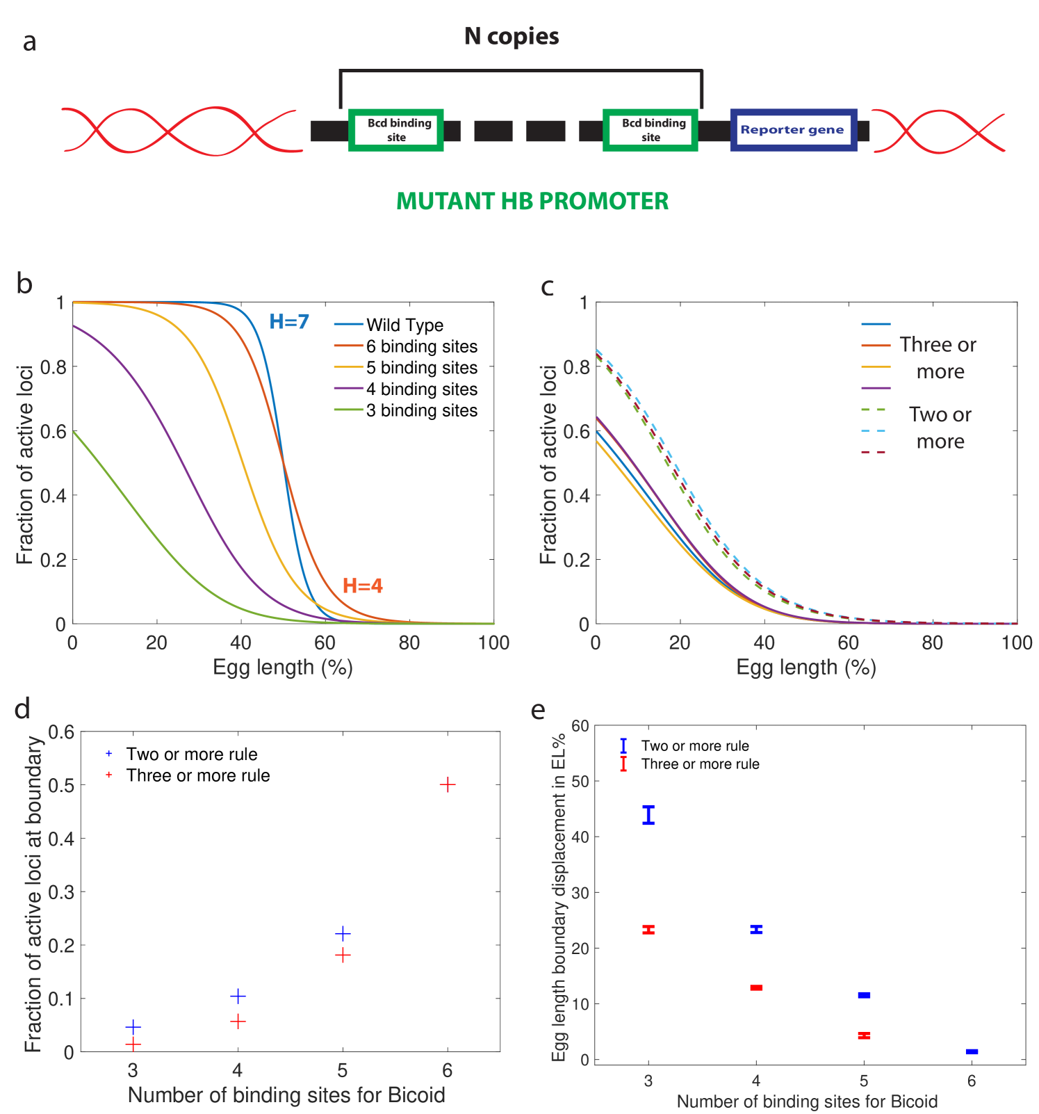
In addition to results for wild type embryos, our approach also yields predictions that could be tested experimentally by using synthetic hb promoters with a variable numbers of Bicoid binding sites (Fig. 6 a). For any of the fast decision-making architectures identified and activation rules chosen, we can compute the effects of reducing the number of binding sites. Specifically, our predictions for the activation rule and in Fig. 6 b can be compared to FISH or fluorescent live imaging measurements of the fraction of active loci at a given position along the anterior-posterior axis. Bcd binding site mutants of the WT promoter have been measured by immunostaining in cycle 14 [53] although mRNA experiments in earlier cell cycles of well characterized mutants are needed to provide for a more quantitative comparison.
An important consideration for the comparison to experimental data is that there is a priori no reason for the hb promoter to have an optimal architecture. We do find indeed many architectures that satisfy all the experimental constraints and are not the fastest decision-making but "good enough" hb promoters. A relevant question then is whether or not similarity in performance is associated with similarity in the microscopic architecture. This point is addressed in Fig. 6c, where we compare the fraction of active loci along the AP axis using several constraint-conforming architectures for and the and activation rules. The plot shows that solutions corresponding to the same activation rule are clustered together and quite distinguishable from the rest. This result suggests that the precise values of the binding and unbinding constants are not important for satisfying the constraints, that many solutions are possible, and that FISH or MS2 imaging experiments can be used to distinguish between different activation rules. The fraction of active loci in the boundary region is an even simpler variable that can differentiate between different activation rules (Fig. 6d). Lastly, we make a prediction for the displacement of the anterior-posterior boundary in mutants, showing that a reduced numbers of Bcd sites results in a strong anterior displacement of the hb expression border compared to binding sites, regardless of the activation rule (Fig. 6e). Error bars in Fig. 6e, that correspond to different close-to-fastest architectures, confirm that these share similar properties and different activation rules are distinguishable.
3 Discussion
The issue of precision in the Bicoid readout by the hunchback promoter has a long history [55, 56]. Recent interest was sparked by the argument that the amount of information at the hunchback locus available during one nuclear cycle is too small for the observed EL distance between neighbouring nuclei that are able to make reproducible distinct decisions [12]. By using updated estimates of the biophysical parameters [13, 34], and the Berg-Purcell error estimation, we confirm that establishing a boundary with variability between neighbouring nuclei would take at least about minutes – roughly the non-transient expression time in nuclear cycle 14 [8, 34] (Appendix A). This holds for a single Bicoid binding site. An intuitive way to achieve a speed up is to increase the number of binding sites: multiple occupancy time traces are thereby made available, which provides a priori more information on the Bicoid concentration.
Possible advantages of multiple sites are not so easy to exploit, though. First, the various sites are close and their respective bindings are correlated [19], so that their respective occupancy time traces are not independent. That reduces the gain in the amount of information. Second, if the activation of gene expression requires the joint binding of multiple sites, the transition to the active configuration takes time. The overall process may therefore be slowed down with respect to a single binding site model, in spite of the additional information. Third, and most importantly, information is conveyed downstream via the expression level of the gene, which is again a single time trace. This channeling of the multiple sites’ occupancy traces into the single time trace of gene expression makes gene activation a real information bottleneck for concentration readout. All these factors can combine and even lead to an increase in the decision time. To wit, an all-or-nothing equilibrium activation model with six identical binding sites functioning at the diffusion limit and no cooperativity takes about minutes to achieve the same above accuracy. In sum, the binding site kinetics and the gene activation rules are essential to harness the potential advantage of multiple binding sites.
Our work addresses the question of which multisite promoters architecture minimize the effects of the activation bottleneck. Specifically, we have shown that decision schemes based on continuous updating and variable decision times significantly improve speed while maintaining the desired high readout accuracy. This should be contrasted to previously considered fixed-time integration strategies. In the case of the hunchback promoter in the fly embryo, the continuous update schemes achieve the EL positional resolution in less than 1 minute, always outperforming fixed-time integration strategies for the same promoter architecture (see SI Table 1). While 1 minute is even beyond what is required for the fly embryo, this margin in speed allows to accommodate additional constraints, viz. steep spatial boundary and biophysical constraints on kinetic parameters. Our approach ultimately yields many promoter architectures that are consistent with experimental observables in fly embryos, and results in decision times that are compatible with a precise readout even for the fast nuclear cycle 11 [8, 34].
Several arguments have been brought forward to suggest that the duration of a nuclear cycle is the limiting time period for the readout of Bicoid concentration gradient. The first one concerns the reset of gene activation and transcription factor binding during mitosis. In that sense, any information that was stored in the form of Bicoid already bound to the gene is lost. The second argument is that the hunchback response integrated over a single nuclear cycle is already extremely precise. However, none of these imply that the hunchback decision is made at a fixed time (corresponding to mitosis) so that strategies involving variable decision times are quite legitimate and consistent with all the known phenomenology.
We have performed our calculations in a worst-case scenario. First, we did not consider averaging of the readout between neighbouring nuclei. While both protein [23] and mRNA concentrations [57] are definitely averaged, and it has been shown theoretically that averaging can both increase and decrease [24] readout variability between nuclei, we do not take advantage of this option. The fact that we achieve less than three minutes in nuclear cycle 11, demonstrates that averaging is a priori dispensable. Second, we demand that the hunchback promoter results in a readout that gives the positional resolution observed in nuclear cycle 14, in the time that the hunchback expression profile is established in nuclear cycle 11. The reason for this choice is twofold. On the one hand, we meant to show that such a task is possible, making feasible also less constrained set-ups. On the other hand, the hunchback expression border established in nuclear cycle 11 does not move significantly in later nuclear cycles in the WT embryo, suggesting that the positional resolution in nuclear cycle 11 is already sufficient to reach the precision of later nuclear cycles. The positional resolution that can be observed in nuclear cycle 11 at the gene expression level is EL [34], but this is also due to smaller nuclear density.
Two main factors generally affect the efficiency of decisions: how information is transmitted and how available information is decoded and exploited. Decoding depends on the representation of available information. Our calculations have considered the issue of how to convey information across the bottleneck of gene activation, under the constraint of a given Hill coefficient. The latter is our empirical way of taking into account the constraints imposed by the decoding process. High Hill coefficients are a very convenient way to package and represent positional information: decoding reduces to the detection of a sharp transition, an edge in the limit of very high coefficients. The interpretation of the Hill coefficient as a decoding constraint is consistent with our results that an increase in the coefficient slows down the decision time. The resulting picture is that promoter architecture results from a balance between the constraints imposed by a quick and accurate readout and those stemming from the ease of its decoding. The very possibility of a balance is allowed by the main conclusion demonstrated here that promoter structures can go significantly below the time limit imposed by the duration of the early nuclear cycles. That leaves room for accommodating other features without jeopardising the readout timescale. While the constraint of a fixed Hill coefficient is an effective way to take into account constraints on decoding, it will be of interest to explore in future work if and how one can go beyond this empirical approach. That will require developing a joint description for transmission and decoding via an explicit modeling of the mechanisms downstream of the activation bottleneck.
Recent work has shed light on the role of out of equilibrium architectures on steepness of response [45] and gradient establishment [34, 53]. Here, we showed that equilibrium architectures perform very well and achieve short decision times, and that out of equilibrium architectures do not seem to significantly improve the performance of promoters, except for making some switches from gene states a bit faster. Non-equilibrium effect can, however, increase the Hill coefficient of the response without adding extra binding sites, which is useful for the downstream readout of positional information that we formulated above as decoding.
We also showed how short bound times of Bicoid molecules to the DNA [52] are translated into accurate and fast decisions. Our fast decision-making architectures also display short DNA-bound times. However, the constraint of high cooperativity means that the distribution of bound times to the DNA is non-exponential and the rare long binding times that occur during the bursty binding process are exploited during the read-out. The combination of high cooperativity and high temporal variance due to bursty dynamics is a possible recipe for an accurate readout.
At the technical level, we developed new methods for the mean decision time of complex gene architectures within the framework of variable time decision-making (SPRT). This allowed us to establish the equality between drift and diffusion of the log-likelihood between two close hypotheses. Its underlying reason is the martingale property that the conditional expectation of probabilities for two hypotheses, given all prior history, is equal to their present value. The methodology developed here will be useful for the broad range of decision processes where SPRT is relevant. The general rules for building efficient readout mechanisms that we discussed here could be relevant for synthetic biology.
Finally, we made predictions about how promoter architectures with different activation schemes can be compared in synthetic embryos with different numbers of Bcd binding sites. Furthermore, experiments that change the composition of the syncytial medium would influence the diffusion constant and assay the assumption of diffusion-limited activation. Our model predicts that these changes would result in modifications of hunchback activation profiles: higher or lower diffusion rates slide the hunchback profile towards the anterior or the posterior end of the embryo, respectively, similarly to an increase or a decrease of the number of Bicoid binding sites. Any of the above experiments would greatly advance our understanding of the molecular control of spatial patterning in Drosophila embryo and, more generally, of regulatory processes.
Acknowledgements: We are grateful to Gautam Reddy and Huy Tran for multiple relevant discussions.
Appendix A Biological parameters in the embryo
To build a model of the promoter, we combine parameters from recent experimental work.
The embryo at nuclear cycle is modelled as having nuclei/cells. For simplicity we assume they are equidistributed on the periphery of the embryo and across the embryo’s length and do not take into account the effect of the geometry of the embryo because the curvature of the embryo is small (the embryo is about -long along the anterior-posterior axis and only about -long along the Dorso-ventral axis). We also neglect the few nuclei forming pole cells and remaining in the bulk [51].
The Bicoid concentration in the embryo is given by , where is the position along the anterior-posterior (AP) embryo axis measured in of the egg length, is the decay length also measured in of the egg length ( which is roughly of the egg length [12]) and is the position of half-maximum hunchback expression ( is of the order of and varies slightly depending on cell cycle, usually close to egg length for the WT hunchback promoter [13]). is the concentration of free Bicoid molecules at the AP boundary [58] (that also corresponds to the point of largest hunchback expression slope [34]).
To compute the diffusion limited arrival rate at the locus, we use the following parameters: diffusivity [13, 58], concentration of free Bicoid molecules at the AP boundary , size of the binding target [23], which leads to an effective at the boundary. This value is an upper bound, assuming that every encounter between a transcription factor and a binding site results in successful binding. We note in Fig. 4 b that most of the ON rates are close to the diffusion limit. We conclude that in this parameter regime, the most efficient strategy is to have ON events that are as fast as possible. The only reason to reduce them is to achieve the required Hill coefficient. That can be done by either adjusting the ON or the OFF rates.
The above estimate s-1 may be inaccurate for various reasons and we ought to explore the sensitivity of results to those uncertainties. Table 1 recapitulates the time-performance of different strategies for different choices of the parameters. A first source of uncertainty is the value of the diffusivity, which is estimated to vary between and [13, 58]. We consider then two possible values for the diffusivity from [13]: and the aforementioned value . A second source of uncertainty is that the actual Bicoid concentration at the boundary could vary by up to a factor two depending on estimates of the concentration and its decay length [12, 58, 34]. We consider then two possible value for the concentration: the aforementioned molecules per , and molecules per . Finally, we assumed above that the size of the target is the full Bicoid operator site, which we took about ten base pairs following Ref. [23]. However, assuming that the TF must reach a specific position on the promoter binding site could reduce the size of the target to a single base pair, that is by a factor . In terms of parameters, we consider then two possible values for : either , or . All in all, taking into account the various sources of uncertainty can range in the interval .
We consider four possible decision strategies. The first one is a single binding site making a fixed-time decision. This computation is made using the original Berg-Purcell formula [17]. In the Berg-Purcell strategy, the concentration of the ligand is inferred based on the total time that the receptor or the binding site has spent occupied by ligands. Due to averaging, the relative error of the concentration readout is inversely proportional to the number of independent measurements of the concentration that can be made within the total fixed time , i.e. to the arrival rate of new Bicoid molecules at the binding site, multiplied by the probability to find the binding site empty (in our case, at the boundary, the probability is roughly one half). Since the rate of arrival of new Bicoid molecules to the binding site is , the relative error of the concentration readout is given by
| (8) |
where is the estimate of the concentration, is the integration time and is the probability that the binding site is full.
In the second strategy, there are sets of binding sites being read independently. In that case, the information from each binding site can be accessed individually and their contributions averaged to give a more precise estimate. This calculation again can be made using the original Berg-Purcell formula [17] for several receptors, dividing the relative error by the square root of the total number of binding sites in Eq. 8:
| (9) |
where is the total number of binding sites (in our case, ).
For the third possibility, we consider a decision made at a fixed time using the fastest architecture identified (Fig. 4) without constraint on the slope (activation rule ). We compute the decision time using the drift-diffusion approximation with fixed time (see Appendix B).
Finally, we consider the fastest architecture identified with a random decision time and the Sequential Probability Ratio Test (SPRT) strategy.
The result of the above calculations is that for a single receptor estimating Bcd concentration with precision within a fixed-time Berg-Purcell type calculation (see section B), decisions take between min for the fastest binding rates and hours for the slowest estimates. Conversely, by using the on-the-fly SPRT decision-making process and the -or-more scheme at equilibrium, the time needed to make decisions with precision and an error rate of at the boundary is s for the fastest rates and minutes for the slowest rates. For all sets of parameters, the on-the-fly SPRT decision-making process gives a -fold faster decision time than the Berg-Purcell estimate and a -fold faster decision making time than the one-binding-site Berg-Purcell estimate. For the fastest rates, a decision with an error rate of less than can be achieved in about minutes within the SPRT scheme.
| Berg-Purcell one operator site | h | min | min | min | min | min | min | min |
| Berg-Purcell twelve operator sites independently read | min | min | min | min | min | min | min | min |
| Optimal equilibrium architecture fixed-time decision () | min | min | min | min | min | min | min | min |
| Optimal equilibrium architecture SPRT decision () | min | min | min | min | min | s | min | s |
Appendix B Error rate and decision time for the fixed-time decision strategy
In this section we describe how we compute the decision time for a fixed-time strategy (or "Berg-Purcell type decision") and a complex promoter architecture.
The classic Berg-Purcell calculation is based on the idea of averaging the time spent by the ligand bound to a receptor (or, in our case, a binding site). The original calculation assumed that the waiting times between binding and unbinding are exponential and that the bound times are not informative about the concentration. Neither of these assumptions hold in the case of the hunchback promoter. Indeed, in the context of a complex promoter architecture, the waiting times that are available to the nucleus or cell downstream are the gene’s ON and OFF switching times. They are not exponentially distributed, and, depending on the activation rule, the OFF times can be just as informative about the concentration as the ON times. For these two reasons, we ought to readapt the Berg-Purcell idea to compute the mean decision time.
To that purpose, we consider a decision with a given rate of error , fix a time of decision and choose the concentration that has the highest likelihood between the two options and . In other words, if then the nucleus chooses , while if then it chooses . For instance, if the actual concentration , then the probability of error at time is given by .
To calculate the above error, we use the drift-diffusion approximation for , compute the drift and diffusivity from Eq. 1-4 and approximate the distribution of by a normal distribution with mean and standard deviation . We compute the error rate for the fixed-time decision process based on the Gaussian approximation. Finally, to find the mean decision time for a given error rate, we perform a quick one-dimensional search over , which yields the value of the fixed decision time appropriate for the prescribed error .
Appendix C The mean first-passage time for the decision-making process
To investigate the role of promoter architectures in decision-making, we apply the SPRT approach (Sequential Probability Ratio Test) [26, 27]. In the simplest formulation of this approach, a decision is made between two hypotheses about the concentration of a surrounding TF: either the TF is at concentration or it is at concentration . The decision is based on the binding and unbinding events of the TF to a promoter. At each point in time, the error of committing to a given concentration (scenario) is estimated by computing the ratio of the probability of one hypothesis, (the surrounding concentration is ) over the other (the concentration is ), :
| (10) |
Technically, the time dependent likelihood ratio, undergoes a random walk as TFs bind and unbind to the promoter, activating and deactivating the gene. The process is terminated and a decision is made when the likelihood ratio falls below the desired error level, which is expressed in terms of absorbing boundaries at (the concentration is ) and (the concentration is ): or (see Fig. 1.1). The boundaries can be expressed in terms of the error and for symmetric errors, [27]. In our case . The mean time for decision can be computed for each discrimination task as the mean first-passage time of a random walk (in the limit of long decision times). In Fig. 7 we show the mean decision-time for different values of .
Assuming the gene has two levels of activation ON and OFF, the information available to downstream mechanisms is a series of ON times and OFF times of gene activity. The probability of a concentration hypothesis is then . If successive ON and OFF times are independent then the probabilities factorize. The log ratio is then written as a function of the ON (respectively OFF) time probability distribution (respectively )
| (11) |
where is the number of ON to OFF switching events and the number of OFF to ON switching events [27]. To understand the dynamics of the log ratio, it is necessary to compute the distributions and based on the promoter dynamics, which is the focus of the following subsection.
C.1 From binding to gene activation
In this section we describe how the high-dimensional complete state of the promoter is mapped onto the low-dimensional activity of the gene. We use a formalism similar to that of Refs. [11, 34].
The promoter features binding sites : its complete state at time is described by an dimensional vector , where if the binding site is empty/full. We assume the gene has two levels of activity: either it is OFF and no mRNA is produced, or it is ON and mRNA is produced at a fixed rate. Activity is then described by a simple Boolean variable equal to , corresponding to the gene being OFF/ON.
We also assume that the activity of the gene depends only on the total number of transcription factors bound to the promoter so that there is an integer such that (where is the indicator function). From the point of view of gene activity, we are only interested in the dynamics of . We make another simplifying assumption: the probabilities of increasing or decreasing only depend on the value of and not on which binding sites specifically are bound or unbound, that is itself has a Markovian dynamics in .
At a given time , we describe the stochastic state of the promoter as a vector of probability where is the probability of having and . The Markovian dynamics of B translate into an transition matrix for : . describes the dynamics of the promoter from the point of view of gene activity. If transcription factors do not dimerize or form complexes, then only if since the probability of two of them binding or unbinding decreases as the square of time for short times.
Let us now relate the statistics of the switching times for the gene activity to the transition matrix . Starting from a distribution of OFF states we compute the cumulative distribution function of the waiting time before switching to the state
| (12) |
where is the transpose, is a vector of for states corresponding to active genes and for states corresponding to inactive genes, and is a modified version of where all ON states act as "sinks" (i.e. all the transition rates from ON states have been set to ). The expression in Eq. 12 computes the cumulative probability of transitions to an ON state before time , that is .
For simplicity, we restrict ourselves to promoter structures where there is only one point of entry into the ON or the OFF states (i.e. any switching event from ON to OFF or vice versa will end with the promoter having a specific number of binding sites). Under this hypothesis, the probability vector in Eq. 12 is uniquely determined and independent of the specific dynamics of the previous ON or OFF times. We relax these constraints on the promoter structure in Appendix G. We denote by (respectively ) the average of the OFF (respectively ON) times for the real concentration .
C.2 Random walk of the log ratio
When the two hypothesized concentrations are very similar to each other as compared to the concentration scale set by the actual concentration value, , the discrimination is hard and requires a large number of binding and unbinding events. In this limit, the random walk can be approximated by a drift-diffusion process with drift and diffusion :
| (13) |
where is a Gaussian white noise. The decision time for the case of symmetric boundaries is a random variable with mean given by Eq. 1 in the main text [27]. depends on the details of the biochemical sensing of the TF concentration and promoter architecture via the drift and diffusivity. Computing and in Eq. 13 is enough to derive the mean first-passage time to the decision and even its full distribution by computing its Laplace transform as a solution of the drift-diffusion equation using standard techniques of first-passage for Gaussian processes [27].
C.3 Drift
For many switching events and , the sums in Eq. 11 can be replaced by continuous averages over binding time distributions. Since and differ at most by one, we can also replace the two values by a unique value , which is the number of ON-OFF cycles. The times are distributed according to the ON and OFF probability distributions for the real concentration . At a given large time , the number of terms in the sum and the log-ratios appearing in Eq. 11 are a priori correlated but Wald’s equality [26] ensures that the average of the sum is the product of the two averages. Since the expected number of cycles grows linearly in time as , we conclude that the drift term in Eq. 13 is given by :
| (14) | ||||
where is the Kullback-Leibler divergence between the two distributions and .
In sum, the drift is determined by how informative the distribution of waiting times in the ON and OFF states are about the concentration differences, with an average rate equal to the inverse of the cycle time . The Kullback-Leibler divergence appearing in Eq. 14 is intuitive : it represents the distance between the real concentration and the hypothetical concentration in the space of probabilistic models of switching times. The larger that distance, the easier it becomes to tell the difference between the two distributions through random sampling.
C.4 Expansion of the drift for small concentration differences
When the two candidate concentrations are similar, , the quantities computed in the previous subsection can be expanded at first order in the differences in concentrations and . Starting from Eq. 14, we expand the drift at first and second orders:
| (15) | ||||
where means that the same operations and integrations are performed for .
Due to conservation of probability, the integral of the first and second -derivatives of vanish. The first-order expansion of vanishes and we have at first non-vanishing order in
| (16) |
If for instance then the drift is positive, favouring the concentration , closer to the real concentration.
C.5 Equality between drift and diffusivity
In this section we present different ways of proving the equality between and in SPRT when the two hypotheses are close by connecting different approaches. We show that this equality is a general property of random walks in Bayesian belief space. We check that these results are true in the controlled case of one binding site in Fig. 8.
First approach: the exit points of the decision process. As proved by Wald in the original paper where he introduced sequential probability ratio tests [59], the nature of the test (the ratio between the likelihood of two hypotheses) requires a specific relationship between the error and the boundaries that define the regions of decision. In our case, we assume the same probability of calling when is true and calling when is true, leading to the definition of only one error level and two symmetric boundaries and . Specifically Wald shows that (see also [27]).
When the two hypotheses are close enough that the variations of the -likelihood can be approximated by a Gaussian process, one can compute the exit probabilities in terms of the drift and diffusivity . The equation for the probability of absorption at the upper boundary is
| (17) |
with the boundary condition and . The corresponding solution is
| (18) |
as shown in the supplementary material of [27]. Setting in Eq. 18, we find that
| (19) |
We note that this probability of absorption is also by definition of the error (assuming for instance that ) leading to
| (20) |
which in turn gives
| (21) |
And so we find that in the limit of close hypotheses, .
Second approach: expansion for small concentration differences. Let us consider the SPRT process between two hypotheses and and assume for simplicity that . In this version of the proof, we consider that the difference is small compared to (i.e ) and expand the expressions for drift and diffusion in increasing orders of to find that they match. We have shown in Appendix C.4 that the first non-vanishing term in the expansion of the drift is of order in and is given by Eq. 16. An integral formula for the second moment of the -likelihood is given in Eq. A15 of [49] from which we get that the diffusivity of the ratio is the sum of four terms. The first term is given by
| (22) |
is proportional to and so is of order . The second term is given by
| (23) | ||||
The prefactor is of order . Expanding the first two terms in the brackets gives the same type of terms as in Eq. 15. Because of probability conservation we find that these terms are of the same order as (i.e ). The last two terms have prefactors and respectively which break the argument for vanishing first order terms in Eq. 15 and these terms are of order . Putting the pieces together, we find that is of order . The third term is given by
| (24) |
Because ON and OFF times are independent, cross terms in are products of two and are of subleading order . Using the symmetry between and we expand one of the square terms in
| (25) | |||
The fourth term is which is of order . So we find that, at leading order, which has the same expansion as (see Eq. 16). And so we recover that for small concentration differences, .
In the case of one binding site with ON rate and OFF rate we check that the formula from [49] gives the exact expression computed in [27]
| (26) |
Replacing with in Eq. 26 and expanding in we have
| (27) | ||||
We identify the drift computed for the one binding site example in 1.2.2 of the main text and find that at first order drift and diffusivity are equal.
Third approach: general properties of Bayesian random walks. To understand the origin of the equality between drift and diffusion, we go back to the definition of SPRT as the update of the Bayesian beliefs in two competing hypotheses. We no longer condition the process on one hypothesis being true but rather on the probability that each one is true given the value of the ratio a certain time point. A very general property of posterior distributions updated with evidence is that their average does not change. This martingale property of belief update can be shown in the following way: assume that the nucleus receives extra evidence with probability . Before that evidence comes, the probability that hypothesis is true has a certain distribution . Then we have that the probability that hypothesis is true varies as :
| (28) |
where we used Bayes rule. The integral of over sums up to and we are left with
| (29) |
In the context of two hypothetical concentrations, we consider the normalized likelihood of the two hypotheses at time : and , where is the likelihood that hypothesis is true based on the evidence accumulated up to time . The martingale property translates as
| (30) |
where are averages taken assuming hypothesis is true and is the variation of through time (or accumulated evidence). We note that and , where is the -likelihood ratio at a given time. We express the variations of the probabilities in terms of the -likelihood so that we can connect it to the drift-diffusion parameters. The drift and diffusivity that depend a priori on the real concentration are respectively the average and variance of the variation of . We have , , and (where is the total change over time ). When the two concentrations are close, the statistics of the acquisition of evidence are symmetric for and and we get that and . As explained in subsection 1.2.2 of the main text, computing the derivatives of with respect to is straightforward. Plugging these relationships into Eq. 30 and gathering terms in and we find that
| (31) | ||||
from which we derive that .
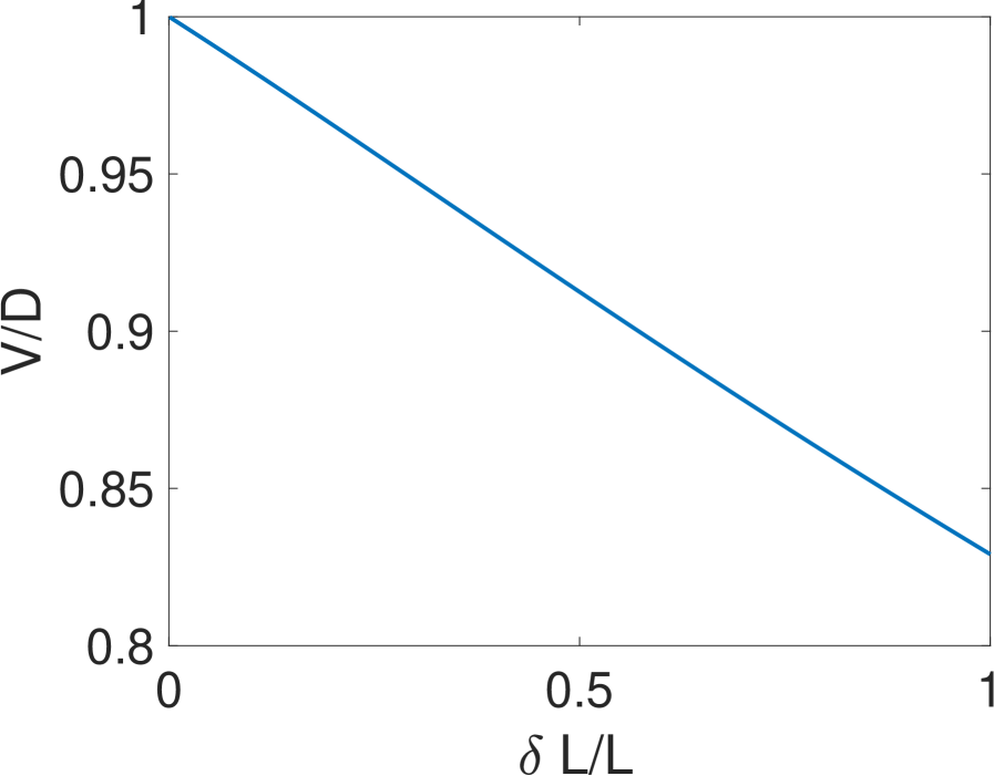
C.6 The first passage time to decision
The first exit time of a drift-diffusion process starting from with two symmetric boundaries at and is given by (see for instance [46]). Plugging in , we recover Eq. 4 of the main text:
| (32) |
We check that this approximation is correct for small concentration differences in Fig. 9 a, b and c. As mentioned in the main text, because the hyperbolic tangent is very flat for high values of its argument, we find that the mean decision time depends weakly on corrections to when the error rate is small (which is equivalent to large). We check that this result in true in Fig. 9 d. We note that from we have . And so we recover the second part of Eq. 4 from the main text
| (33) |
In one of the original papers about SPRT [26], Wald derives a similar formula for the total number of events before the decision:
| (34) |
where is the number of ON-OFF events when decision happens. Combining Eq. 34 with Wald’s equality [47, 48] that states that we recover Eq. 33.
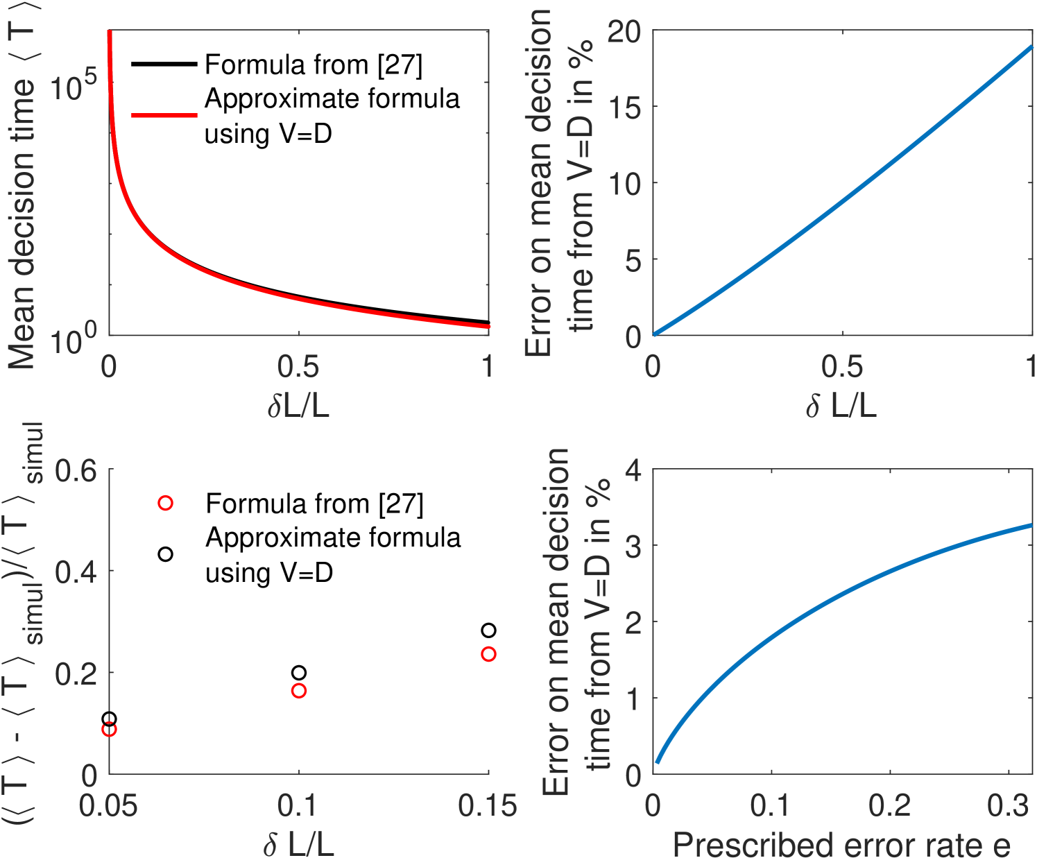
C.7 When are correlations between the times of events leading to decision important?
To compute the drift or diffusivity, one must compute the variation of the -likelihood up to a given time . The fact that the total time is fixed introduces correlation between the duration of the different ON-OFF events. Can these correlations be ignored, leading to an effective drift or diffusion per cycle? They can only when the two concentrations are close, as we check in Fig. 10.
Following the arguments in [49], let us consider the following generating function for the cumulants of the log-likelihood difference at a given time assuming hypothesis is true ( or ) :
| (35) |
where is the -likelihood of hypothesis , is the number of ON-OFF cycles and and are respectively the ON and OFF waiting times. This is not exactly what appears in [49] but it is sufficient to grasp the consequences of the correlations introduced by a global constraint on the duration of the process, i.e. the function. Note that such constraint breaks the statistical independence of the various cycles, and introduces dependencies even though the and factorize. We rewrite the Heaviside function using the Laplace transform form and the product of the probabilities as , where and are the log-likelihoods for hypothesis . Putting the pieces together we obtain
| (36) |
where
| (37) |
One can remark that the expression is factorized, i.e. is raised to the power , and even itself can be interpreted as "expectation value" of (and same with ) over the "distribution" , i.e. the constraint introduces an exponential factor that distorts the weight of the various durations. These elements are consistent with the idea of a random variable per cycle that can be averaged to compute the drift and diffusivity. However, the idea of ignoring correlations between duration of events is not valid because is a function of . Indeed, summing the series over gives and the asymptotic behavior is then determined by the first singularity encountered as is moved to the left for the inverse Laplace transform. For each value of , this determines a value of , that is (see [49] for the complete calculation).
What the above says more qualitatively is that the variables per cycle are correlated because of the global constraint and there is not a single-cycle effective probability distribution that can account for that because of the dependence of on . In other words, different moments involve different configurations and distortions of the weights for the durations of the cycles. The only exception is when vanishes, which is the case for two close hypotheses. Indeed, from , one obtains and it also holds . We checked explicitly in subsection C.5 that in that limit in the formula from [49] the first two terms are negligible and the diffusivity reduces to the variance of the log-likelihoods only.
Indeed, when the two hypothetical concentrations are close and the correlations can be ignored, a diffusivity per cycle can be defined naturally as
| (38) |
where is the average of the squared -likelihood variation (see Eq. 24). We check in Fig. 10 that this formula is a good approximation for small concentration differences in the context of one binding site. In that context we have
| (39) |
where is the OFF rate and is the ON rate. We find that this approximation is better than the approximation only when the cycle times depend weakly on the concentration (i.e, for one binding site, when is small, see Fig. 10).
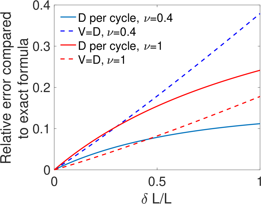
Appendix D The mean first-passage time for different architectures
Activation by multiple TF - irreversible binding all-or-nothing models. We first consider the all-or-nothing two binding site cycle model depicted in Fig. 5 a.
In this model, ON events end when the complex formed by two copies of the TF unbinds. It follows that ON times are exponentially distributed and independent of the concentration . Because they are independent of the concentration, they will not contribute to the log ratios. The mean ON time is given by .
The activation time (OFF time) requires two copies of the TF to bind and is the sum of the times it takes for each of them to bind. From a probabilistic point of view, this sum becomes a convolution and the OFF times are given by
| (40) | ||||
The average OFF time is .
We can now compute the drift (the ON times do not contribute to information)
| (41) | ||||
The calculations above are only valid when the two binding rates are different . Let us now assume that . The ON time distribution is unchanged but the OFF time distribution is now
| (42) |
where we have identified , the standard Gamma distribution with exponent and parameter . The expression of the drift simplifies as :
| (43) | ||||
When the two binding rates and are similar but not exactly equal the activation time distribution can be approximated by the Gamma distribution . It is then convenient to use Eq. 43 with as a parameter.
Activation by multiple TF – irreversible binding with -or-more activation. We now consider the non-equilibrium two binding site -or-more activation model depicted in Fig. 5 b. The OFF times are exponentially distributed . They will contribute as in the one binding-site exponential model.
The ON times are now a convolution of a concentration-dependent exponential step with rate and a concentration-independent unbinding with rate . Their distribution is
| (44) |
The expression is valid for and, as previously, reduces to a distribution with exponent in case of equality.
The corresponding drift is
| (45) | ||||
Appendix E All-or-nothing vs -or-more activation
In this section we give a more detailed derivation of the result given in section 2.1.4 of the main text. Specifically, we compare two activation rules for the same promoter architecture: two binding sites with binding rates and . We consider that the two binding sites bind TF independently so that (there are two free targets for the first binding). The two copies of the TF unbind together with unbinding rate . It is a cycle model. We consider the -or-more activation rule (Fig. 5b) and the all-or-nothing activation rule (Fig. 5 a). We will prove that the fastest activation scheme is the all-or-nothing scheme when and -or-more when . This result corresponds to the following intuitive idea : given a choice to associate the second binding with either the first binding or the unbinding for the readout by the cell, it is more informative to convolve it with the fastest of the rates to maximize the information extracted from it. This is in general true if the time per cycle is the same for the different architectures considered.
The total time it takes to go through a cycle is the same for the two architectures: , so the difference in performance will come from the amount of information extracted per cycle. We are interested in the limit of similar concentrations, i.e. and , . Since and the decision time is inversely proportional to , it is enough to compare (the drift in the all-or-nothing scheme) with (the drift in the -or-more scheme) to determine the fastest architecture.
To compute , we start from Eq. 41, plugging in , and . We expand for :
| (46) | ||||
where is the Riemann zeta function. Eventually we have
| (47) |
While the expansion of does not take a simple form in general, it can be computed for the specific value of . When , and , expanding to second order Eq. 45 becomes
| (48) | ||||
We can now use the above equality and the following arguments to reach the conclusion stated at the beginning of the section. is independent of because no information is gained about the concentrations from the step involving unbinding. Conversely, is an increasing function of : as decreases, the unbinding part takes over in the convolution for the ON times. Since the difference between the two convolutions can only decrease as decreases, it becomes harder and harder to differentiate the two ON time distributions, their Kullback-Leibler divergence becomes smaller, and the drift term is reduced.
In sum, for , ; is independent of whilst increases with . We conclude that for , and the -or-more scheme is preferred. Conversely, for , and the all-or-nothing scheme is preferred.
Appendix F Comparing one and two binding-site architectures
In this section we compare the performance of a one binding-site architecture (Fig. 5 d) to that of an equilibrium all-or-nothing two binding-site architecture (Fig. 5 c). The motivation is to provide detailed explanations for the results given in subsection 2.1.5 of the main text. To rank their performance, we compare, as in the previous appendix E, the drift for the two architectures.
To do the comparison, we optimize the two binding site architecture rates , and for a fixed value of the error rate , the real concentration , the hypothetical concentrations and and the second unbinding rate . The fixed second unbinding rate sets a time scale for the process. For concreteness, we suppose that the real concentration and decision is hard , .
Decisions can be trivially sped up by increasing indefinitely all the rates to very high values. To avoid this, in the optimization process we set an upper bound to be . We choose this upper bound to be smaller than the largest values of considered () and larger than the smaller values of considered (). From a biological point of view, this upper bound for the ON rates can correspond to the diffusion limited arrival rate. For the OFF rates, it can correspond to a minimum bound time required to trigger a downstream mechanism (for instance, the activation of the gene). We check in Fig. 12 that curves and effects similar to those discussed below are obtained if the upper bounds are modified.
For all values of parameters, we find that the optimal ON rates are maximal (). We observed and discussed in subsection 2.1.5 that for certain values of the parameters ( and ), the optimal first unbinding rate reaches the upper bound while for smaller values the optimal first unbinding rate remains at (Fig 5 inset). The transition between the two regions is sharp. Setting to is equivalent to having an effective one binding site model because the promoter never goes back to the state. For that reason we want to compare the performance of a two binding site model with parameters , , and to that of a one binding site model with parameters and .
Since we are in the limit of small concentration differences, the speed of decision is set by and . We denote the mean drifts of the one and the two binding-site models as and , respectively. Similarly, and are the mean times per cycle of the two models.
The one binding-site architecture activates with rate and deactivates with rate . Both waiting times for ON and OFF expression states are exponential. Following results in subsection 1.2.2 of the main text, we have and . We conclude that :
| (49) |
In the two binding site architecture, the ON times are exponentially distributed with rate . The OFF times are more complex as they can result from several cycles from a promoter with a binding site occupied to an empty promoter before finally switching to two full binding sites and gene activation. We compute using the modified transition matrix of the Markov chain with the ON states acting as sinks as described in Appendix C. The OFF time distribution is given by the derivative of Eq. 12.
In the two binding site model, the transition matrix is a by matrix and can be diagonalized analytically to compute explicitly the exponential in Eq. 12. We set since it is always the case in the identified optimal architectures for the two binding site model (where is the specific value of for which upper bounds on and are equal, in Fig 5 f). We compute the distribution of the OFF times explicitly and find
| (50) |
where .
Computing the mean of the distribution in Eq. 50, we find that the average time for a cycle in the two binding site architecture is
| (51) |
We can now numerically integrate . We use this simplified formula to compare the performance of the two architectures and recover the results of Fig. 5 f. We show an example for a specific value of , varying in Fig 11.
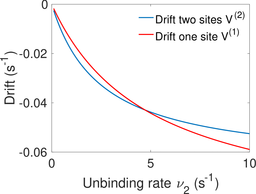
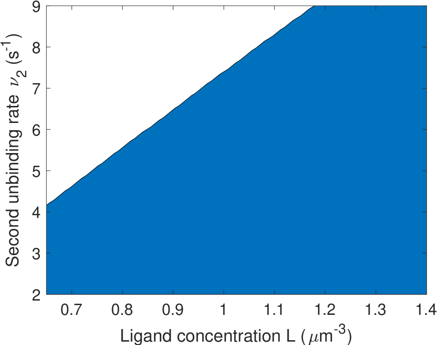
Appendix G Out of equilibrium architectures and averaging over several steps
In some architectures where several copies of the TF can bind or unbind at once, there can be correlations between successive ON and OFF times. This depends on the structure of the promoter Markov chain. It is made of OFF and ON states. There can be correlations between the OFF and ON times if the chain can enter the ON state subgraph through different ON states, coming from different OFF states (or the same situation reverting ON and OFF states). In that case the time that the chain will spend in the ON state will depend on the initial entry state, and so it will depend on the OFF state from which the chain entered the ON subgraph, giving a correlation with the previous OFF time to the ON time. If the structure is particularly complex, these correlations can span over several ON-OFF cycle. We do however assume that the chain is ergodic so that they vanish at long times.
To deal with this situation, a solution is to average the contribution to the information of ON/OFF events over several ON/OFF times, until the correlation with the initial times is lost. The event in the log ratio becomes a series of ON and OFF times and their joint probability (as they no longer factorize). The next series of events can be considered approximately (or exactly in certain cases) independent of the previous series and the rest of the theory can be applied to this sum of independent variables.
We did not explore these architectures in detail as they are extremely complex, do not seem to increase the performance of the promoter for the readout, and most likely the type of information about the concentration that is hidden in the correlation between ON and OFF would be very hard to decode for downstream mechanisms.
Appendix H Parameters for Fig. 6
Parameters for Fig.5 panel a, panel b blue full line, panel c red and panel d red are those identified as optimal for , : , , , , , , , , , , , .
Parameters for Fig.5 panel b green dashed line, panel c blue and panel d blue are those identified as optimal for , : , , , , , , , , , , , .
Other lines in panel b correspond to architectures that are close to optimality, with parameters in the same range as the ones given above.
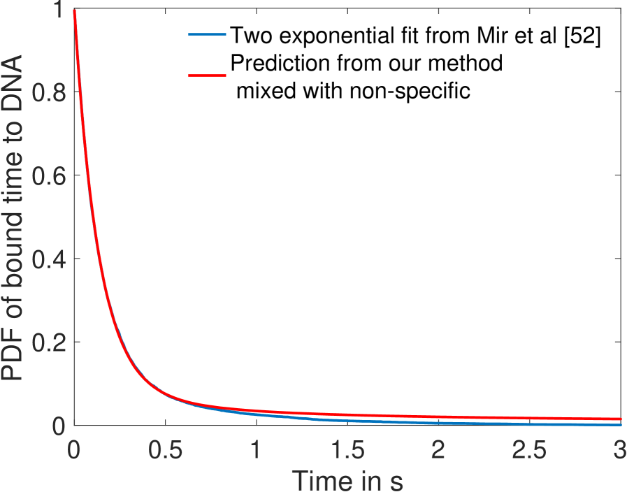
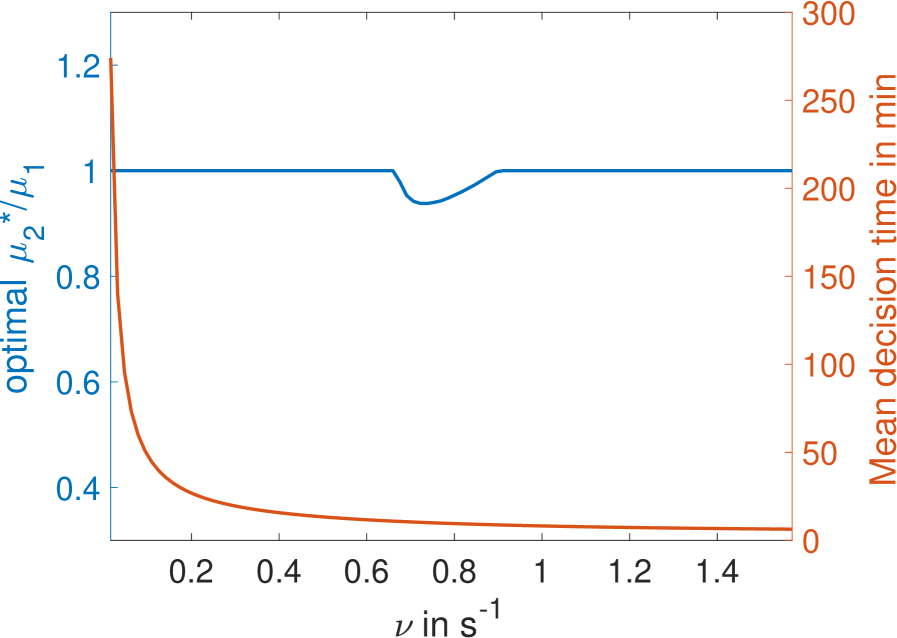
References
- [1] Bahram Houchmandzadeh, Eric Wieschaus, and Stanislas Leibler. Establishment of developmental precision and proportions in the early drosophila embryo. Nature, 415:798 EP –, 02 2002.
- [2] Michael W. Perry, Jacques P. Bothma, Ryan D. Luu, and Michael Levine. Precision of hunchback expression in the Drosophila embryo. Current Biology, 22(23):2247–2252, 2012.
- [3] Kosuke Takeda, Danying Shao, Micha Adler, Pascale G Charest, William F Loomis, Herbert Levine, Alex Groisman, Wouter-Jan Rappel, and Richard A Firtel. Incoherent feedforward control governs adaptation of activated ras in a eukaryotic chemotaxis pathway. Science signaling, 5(205):ra2–ra2, 01 2012.
- [4] John F. Marcelletti and David H. Katz. Antigen concentration determines helper t cell subset participation in ige antibody responses. Cellular Immunology, 143(2):405–419, 1992.
- [5] Clive G Bowsher and Peter S Swain. Environmental sensing, information transfer, and cellular decision-making. Current Opinion in Biotechnology, 28:149–155, 2014.
- [6] Patrick H O’Farrell. Growing an Embryo from a Single Cell: A Hurdle in Animal Life. Cold Spring Harbor Perspectives in Biology, 7(11), nov 2015.
- [7] Patrick H. O’Farrell, Jason Stumpff, and Tin Tin Su. Embryonic cleavage cycles: How is a mouse like a fly? Current Biology, 14(1):R35 – R45, 2004.
- [8] Tanguy Lucas, Huy Tran, Carmina Angelica Perez Romero, Aurélien Guillou, Cécile Fradin, Mathieu Coppey, Aleksandra M Walczak, and Nathalie Dostatni. 3 minutes to precisely measure morphogen concentration. PLoS Genet, 14(10):e1007676, Oct 2018.
- [9] C. Nüsslein-Volhard, E. Wieschaus, and H. Kluding. Mutations affecting the pattern of the larval cuticle indrosophila melanogaster. Wilhelm Roux’s archives of developmental biology, 193(5):267–282, 1984.
- [10] Johannes Jaeger. The gap gene network. Cellular and Molecular Life Sciences, 68(2):243–274, 2011.
- [11] Jonathan Desponds, Huy Tran, Teresa Ferraro, Tanguy Lucas, Carmina Perez Romero, Aurelien Guillou, Cecile Fradin, Mathieu Coppey, Nathalie Dostatni, and Aleksandra M Walczak. Precision of readout at the hunchback gene: Analyzing short transcription time traces in living fly embryos. PLoS Computational Biology, 2016.
- [12] Thomas Gregor, Eric F Wieschaus, Alistair P McGregor, William Bialek, and David W Tank. Stability and nuclear dynamics of the bicoid morphogen gradient. Cell, 130(1):141–52, 2007.
- [13] Aude Porcher, Asmahan Abu-Arish, Sébastien Huart, Baptiste Roelens, Cecile Fradin, and Nathalie Dostatni. The time to measure positional information: maternal hunchback is required for the synchrony of the Bicoid transcriptional response at the onset of zygotic transcription. Development, 137(16):2795–804, 2010.
- [14] Hernan G Garcia, Mikhail Tikhonov, Albert Lin, and Thomas Gregor. Quantitative imaging of transcription in living Drosophila embryos links polymerase activity to patterning. Current Biology, 23(21):2140–5, 2013.
- [15] Mariela D. Petkova, Gašper Tkačik, William Bialek, Eric F. Wieschaus, and Thomas Gregor. Optimal decoding of cellular identities in a genetic network. Cell, 176(4):844–855.e15, 2019.
- [16] Mikhail Tikhonov, Shawn C Little, and Thomas Gregor. Only accessible information is useful : insights from patterning Subject Category :. Royal Society Open Science, 2(150486), 2015.
- [17] H C Berg and E M Purcell. Physics of chemoreception. Biophysical journal, 20(2):193–219, November 1977.
- [18] William Bialek and Sima Setayeshgar. Physical limits to biochemical signaling. Proceedings of the National Academy of Sciences, 2005(102):10040–10045, 2005.
- [19] Kazunari Kaizu, Wiet De Ronde, Joris Paijmans, Koichi Takahashi, and Filipe Tostevin. The Berg-Purcell Limit Revisited. Biophysical journal, 106(4):976–985, 2014.
- [20] Robert G. Endres and Ned S. Wingreen. Accuracy of direct gradient sensing by single cells. Proceedings of the National Academy of Sciences, 105(41):15749–15754, 2008.
- [21] Robert G. Endres and Ned S. Wingreen. Maximum likelihood and the single receptor. Phys. Rev. Lett., 103:158101, Oct 2009.
- [22] Thierry Mora and Ned S. Wingreen. Limits of sensing temporal concentration changes by single cells. Phys. Rev. Lett., 104:248101, Jun 2010.
- [23] Thomas Gregor, David W. Tank, Eric F. Wieschaus, and William Bialek. Probing the limits to positional information. Cell, 130(1):153–164, 2007.
- [24] Thorsten Erdmann, Martin Howard, and Pieter Rein ten Wolde. Role of spatial averaging in the precision of gene expression patterns. Physical Review Letters, 103(25):258101, 2009.
- [25] Gerardo Aquino, Ned S. Wingreen, and Robert G. Endres. Know the single-receptor sensing limit? think again. Journal of Statistical Physics, 162(5):1353–1364, 2016.
- [26] A Wald. Sequential tests of statistical hypotheses. Ann Math Stat, 1945.
- [27] Eric D Siggia and Massimo Vergassola. Decisions on the fly in cellular sensory systems. Proceedings of the National Academy of Sciences, 2013.
- [28] Joshua I. Gold and Michael N. Shadlen. The neural basis of decision making. Annual Review of Neuroscience, 30(1):535–574, 2019/01/23 2007.
- [29] James A. R. Marshall, Rafal Bogazc, Anna Dornhaus, Robert Planque, Tim Kovacs, and Nigel R. Franks. On optimal decision-making in brains and social insect colonies. Journals of the Royal Society Interface, 2009.
- [30] Édgar Roldán, Izaak Neri, Meik Dörpinghaus, Heinrich Meyr, and Frank Jülicher. Decision making in the arrow of time. Physical Review Letters, 115(25):250602–, 12 2015.
- [31] Amanda Ochoa-Espinosa, Danyang Yu, Aristotelis Tsirigos, Paolo Struffi, and Stephen Small. Anterior-posterior positional information in the absence of a strong bicoid gradient. Proceedings of the National Academy of Sciences, 106(10):3823, 03 2009.
- [32] Gerardo Jiménez, Antoine Guichet, Anne Ephrussi, and Jordi Casanova. Relief of gene repression by torso rtk signaling: role of capicua in drosophila terminal and dorsoventral patterning. Genes & Development, 14(2):224–231, 01 2000.
- [33] Thomas R. Sokolowski, Thorsten Erdmann, and Pieter Rein ten Wolde. Mutual repression enhances the steepness and precision of gene expression boundaries. PLOS Computational Biology, 8(8):e1002654–, 08 2012.
- [34] Huy Tran, Jonathan Desponds, Carmina Angelica Perez Romero, Mathieu Coppey, Cecile Fradin, Nathalie Dostatni, and Aleksandra M. Walczak. Precision in a rush: Trade-offs between reproducibility and steepness of the hunchback expression pattern. PLOS Computational Biology, 14(10):e1006513–, 10 2018.
- [35] Michael W Perry, Alistair N Boettiger, and Michael Levine. Multiple enhancers ensure precision of gap gene-expression patterns in the Drosophila embryo. Proceedings of the National Academy of Sciences, 108(33):1–12, 2011.
- [36] Cheryll Tickle Lewis Wolpert and Alfonso Martinez Arias. Principles of development Fifth Edition. Oxford University Press, 2015.
- [37] Wolfgang Driever and Christiane Nüsslein-Volhard. The bicoid protein determines position in the drosophila embryo in a concentration-dependent manner. Cell, 54(1):95–104, 1988.
- [38] Gary Struhl, Paul Johnston, and Peter A. Lawrence. Control of drosophila body pattern by the hunchback morphogen gradient. Cell, 69(2):237–249, 1992.
- [39] Olivier Crauk and Nathalie Dostatni. Bicoid determines sharp and precise target gene expression in the Drosophila embryo. Current Biology, 15(21):1888–98, 2005.
- [40] Tanguy Lucas, Teresa Ferraro, Baptiste Roelens, Jose De Las Heras Chanes, Aleksandra M Walczak, Mathieu Coppey, and Nathalie Dostatni. Live imaging of bicoid-dependent transcription in Drosophila embryos. Current Biology, 23(21):2135–9, 2013.
- [41] C Schröder, D Tautz, E Seifert, and H Jäckle. Differential regulation of the two transcripts from the drosophila gap segmentation gene hunchback. The EMBO journal, 7(9):2881–2887, 09 1988.
- [42] Wolfgang Driever, Gudrun Thoma, and Christiane Nüsslein-Volhard. Determination of spatial domains of zygotic gene expression in the drosophila embryo by the affinity of binding sites for the bicoid morphogen. Nature, 340(6232):363–367, 1989.
- [43] Gary Struhl, Kevin Struhl, and Paul M. Macdonald. The gradient morphogen bicoid is a concentration-dependent transcriptional activator. Cell, 57(7):1259–1273, 1989.
- [44] Amanda Ochoa-Espinosa, Gozde Yucel, Leah Kaplan, Adam Pare, Noel Pura, Adam Oberstein, Dmitri Papatsenko, and Stephen Small. The role of binding site cluster strength in bicoid-dependent patterning in drosophila. Proceedings of the National Academy of Sciences of the United States of America, 102(14):4960, 04 2005.
- [45] Javier Estrada, Felix Wong, Angela DePace, and Jeremy Gunawardena. Information Integration and Energy Expenditure in Gene Regulation. Cell, 166(1):234–44, 2016.
- [46] Sidney Redner. A Guide to First-Passage Processes. Cambridge University Press, Cambridge, 2001.
- [47] Abraham Wald. Some generalizations of the theory of cumulative sums of random variables. 16(3):287–293, 1945.
- [48] Rick Durrett. Probability: Theory and Examples. Cambridge University Press, Cambridge, 2010.
- [49] Martín Carballo-Pacheco, Jonathan Desponds, Tatyana Gavrilchenko, Andreas Mayer, Roshan Prizak, Gautam Reddy, Ilya Nemenman, and Thierry Mora. Receptor crosstalk improves concentration sensing of multiple ligands. Physical Review E, 99(2):022423–, 02 2019.
- [50] Gautam Reddy, Antonio Celani, and Massimo Vergassola. Infomax strategies for an optimal balance between exploration and exploitation. Journal of Statistical Physics, 163(6):1454–1476, 2016.
- [51] V. E. Foe and B. M. Alberts. Studies of nuclear and cytoplasmic behaviour during the five mitotic cycles that precede gastrulation in drosophila embryogenesis. Journal of Cell Science, 61(1):31, 05 1983.
- [52] Mustafa Mir, Armando Reimer, Jenna E. Haines, Xiao Yong Li, Michael Steidler, Hernan Garcia, Michael B. Eisen, and Xavier Darzacq. Dense bicoid hubs accentuate binding along the morphogen gradient. Genes and development, 2017.
- [53] Jeehae Park, Javier Estrada, Gemma Johnson, Chiara Ricci-Tam, Meghan Bragdon, Yekaterina Shulgina, Anna Cha, Jeremy Gunawardena, and Angela H. DePace. Dissecting the sharp response of a canonical developmental enhancer reveals multiple sources of cooperativity. bioRxiv, page 408708, 01 2018.
- [54] Jason Gertz, Eric D. Siggia, and Barak A. Cohen. Analysis of combinatorial cis-regulation in synthetic and genomic promoters. Nature, 457:215 EP –, 11 2008.
- [55] Christiane Nüsslein-Volhard and Eric Wieschaus. Mutations affecting segment number and polarity in drosophila. Nature, 287(5785):795–801, 1980.
- [56] Diethard Tautz. Regulation of the drosophila segmentation gene hunchback by two maternal morphogenetic centres. Nature, 332(6161):281–284, 1988.
- [57] Shawn C Little, Mikhail Tikhonov, and Thomas Gregor. Precise developmental gene expression arises from globally stochastic transcriptional activity. Cell, 154(4):789–800, 2013.
- [58] Asmahan Abu-Arish, Aude Porcher, Anna Czerwonka, Nathalie Dostatni, and Cécile Fradin. High mobility of bicoid captured by fluorescence correlation spectroscopy: Implication for the rapid establishment of its gradient. Biophysical Journal, 99(4):33–35, 2010.
- [59] Abraham Wald. On cumulative sums of random variables. Ann. Math. Statist., 15(3):283–296, 1944.