Hybrid RL: Using Both Offline and Online Data Can Make RL Efficient
Abstract
We consider a hybrid reinforcement learning setting (Hybrid RL), in which an agent has access to an offline dataset and the ability to collect experience via real-world online interaction. The framework mitigates the challenges that arise in both pure offline and online RL settings, allowing for the design of simple and highly effective algorithms, in both theory and practice. We demonstrate these advantages by adapting the classical Q learning/iteration algorithm to the hybrid setting, which we call Hybrid Q-Learning or Hy-Q. In our theoretical results, we prove that the algorithm is both computationally and statistically efficient whenever the offline dataset supports a high-quality policy and the environment has bounded bilinear rank. Notably, we require no assumptions on the coverage provided by the initial distribution, in contrast with guarantees for policy gradient/iteration methods. In our experimental results, we show that Hy-Q with neural network function approximation outperforms state-of-the-art online, offline, and hybrid RL baselines on challenging benchmarks, including Montezuma’s Revenge.
1 Introduction
Learning by interacting with an environment, in the standard online reinforcement learning (RL) protocol, has led to impressive results across a number of domains. State-of-the-art RL algorithms are quite general, employing function approximation to scale to complex environments with minimal domain expertise and inductive bias. However, online RL agents are also notoriously sample inefficient, often requiring billions of environment interactions to achieve suitable performance. This issue is particularly salient when the environment requires sophisticated exploration and a high quality reset distribution is unavailable to help overcome the exploration challenge. As a consequence, the practical success of online RL and related policy gradient/improvement methods has been largely restricted to settings where a high quality simulator is available.
To overcome the issue of sample inefficiency, attention has turned to the offline RL setting [Levine et al., 2020], where, rather than interacting with the environment, the agent trains on a large dataset of experience collected in some other manner (e.g., by a system running in production or an expert). While these methods still require a large dataset, they mitigate the sample complexity concerns of online RL, since the dataset can be collected without compromising system performance. However, offline RL methods can suffer from distribution shift, where the state distribution induced by the learned policy differs significantly from the offline distribution [Wang et al., 2021]. Existing provable approaches for addressing distribution shift are computationally intractable, while empirical approaches rely on heuristics that can be sensitive to the domain and offline dataset (as we will see).
In this paper, we focus on a hybrid reinforcement learning setting, which we call Hybrid RL, that draws on the favorable properties of both offline and online settings. In Hybrid RL, the agent has both an offline dataset and the ability to interact with the environment, as in the traditional online RL setting. The offline dataset helps address the exploration challenge, allowing us to greatly reduce the number of interactions required. Simultaneously, we can identify and correct distribution shift issues via online interaction. Variants of the setting have been studied in a number of empirical works [Rajeswaran et al., 2017, Hester et al., 2018, Nair et al., 2018, 2020, Vecerik et al., 2017] which mainly focus on using expert demonstrations as offline data.
Hybrid RL is closely related to the reset setting, where the agent can interact with the environment starting from a “nice” distribution. A number of simple and effective algorithms, including CPI [Kakade and Langford, 2002], PSDP [Bagnell et al., 2003], and policy gradient methods [Kakade, 2001, Agarwal et al., 2020b] – methods which have inspired recent powerful heuristic RL methods such as TRPO [Schulman et al., 2015] and PPO [Schulman et al., 2017]— are provably efficient in the reset setting. Yet, leveraging a reset distribution is a strong requirement (often tantamount to having access to a detailed simulation) and unlikely to be available in real world applications. Hybrid RL differs from the reset setting in that (a) we have an offline dataset, but (b) our online interactions must come from traces that start at the initial state distribution of the environment, and the initial state distribution is not assumed to have any nice properties. Both features (offline data and a nice reset distribution) facilitate algorithm design by de-emphasizing the exploration challenge. However, Hybrid RL is more practical since an offline dataset is much easier to access, while a nice reset distribution or even generative model is generally not guaranteed in practice.
We showcase the Hybrid RL setting with a new algorithm, Hybrid Q learning or Hy-Q (pronounced: Haiku). The algorithm is a simple adaptation of the classical fitted Q-iteration algorithm (FQI) and it accommodates value-based function approximation in a relatively general setup. 666We use Q-learning and Q-iteration interchangeably, although they are not strictly speaking the same algorithm. Our theoretical results analyze Q-iteration, but we use an algorithm with an online/mini-batch flavor that is closer to Q-learning for our experiments. For our theoretical results, we prove that Hy-Q is both statistically and computationally efficient assuming that: (1) the offline distribution covers some high quality policy, (2) the MDP has low bilinear rank, (3) the function approximator is Bellman complete, and (4) we have a least squares regression oracle. The first three assumptions are standard statistical assumptions in the RL literature while the fourth is a widely used computational abstraction for supervised learning. No computationally efficient algorithms are known under these assumptions in pure offline or pure online settings, which highlights the advantages of the hybrid setting.
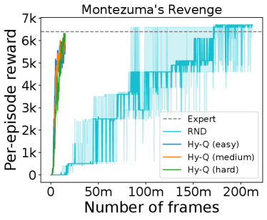
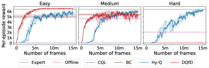
We also implement Hy-Q and evaluate it on two challenging RL benchmarks: a rich observation combination lock [Misra et al., 2020] and Montezuma’s Revenge from the Arcade Learning Environment [Bellemare et al., 2013]. Starting with an offline dataset that contains some transitions from a high quality policy, our approach outperforms: an online RL baseline with theoretical guarantees, an online deep RL baseline tuned for Montezuma’s Revenge, a pure offline RL baseline, an imitation learning baseline, and an existing hybrid method. Compared to the online methods, Hy-Q requires only a small fraction of the online experience, demonstrating its sample efficiency (e.g., Figure 1). Compared to the offline and hybrid methods, Hy-Q performs most favorably when the offline dataset also contains many interactions from low quality policies, demonstrating its robustness. These results reveal the significant benefits that can be realized by combining offline and online data.
2 Related Works
We discuss related works from four categories: pure online RL, online RL with access to a reset distribution, offline RL, and prior work in hybrid settings. We note that pure online RL refers to the setting where one can only reset the system to initial state distribution of the environment, which is not assumed to provide any form of coverage.
Pure online RL
Beyond tabular settings, many existing statistically efficient RL algorithms are not computationally tractable, due to the difficulty of implementing optimism. This is true in the linear MDP [Jin et al., 2020] with large action spaces, the linear Bellman complete model [Zanette et al., 2020, Agarwal et al., 2019], and in the general function approximation setting [Jiang et al., 2017, Sun et al., 2019, Du et al., 2021, Jin et al., 2021a]. These computational challenges have inspired results on intractability of aspects of online RL [Dann et al., 2018, Kane et al., 2022]. On the other hand, many simple exploration based algorithms like -greedy are computationally efficient, but they may not always work well in practice. Recent theoretical works [Dann et al., 2022, Liu and Brunskill, 2018] have explored the additional structural assumptions on the underlying dynamics and value function class under which -greedy succeeds, but they still do not capture all the relevant practical problems.
There are several online RL algorithms that aim to tackle the computational issue via stronger structural assumptions and supervised learning-style computational oracles [Misra et al., 2020, Sekhari et al., 2021, Zhang et al., 2022c, Agarwal et al., 2020a, Uehara et al., 2021, Modi et al., 2021, Zhang et al., 2022a, Qiu et al., 2022]. Compared to these oracle-based methods, our approach operates in the more general “bilinear rank” setting and relies on a standard supervised learning primitive: least squares regression. Notably, our oracle admits efficient implementation with linear function approximation, so we obtain an end-to-end computational guarantee; this is not true for prior oracle-based methods.
There are many deep RL methods for the online setting (e.g., Schulman et al. [2015, 2017], Lillicrap et al. [2016], Haarnoja et al. [2018], Schrittwieser et al. [2020]). Apart from a few exceptions (e.g., Burda et al. [2018], Badia et al. [2020], Guo et al. [2022]), most rely on random exploration (e.g. -greedy) and are not capable of strategic exploration. In fact, guarantees for -greedy like algorithms only exist under additional structural assumptions on the underlying problem.
In our experiments, we test our approach on Montezuma’s Revenge, and we pick Rnd [Burda et al., 2018] as a deep RL exploration baseline due to its simplicity and effectiveness on the game of Montezuma’s Revenge.
Online RL with reset distributions
When an exploratory reset distribution is available, a number of statistically and computationally efficient algorithms are known. The classic algorithms are Cpi [Kakade and Langford, 2002], Psdp [Bagnell et al., 2003], Natural Policy Gradient [Kakade, 2001, Agarwal et al., 2020b], and PolyTex [Abbasi-Yadkori et al., 2019]. Uchendu et al. [2022] recently demonstrated that algorithms like Psdp work well when equipped with modern neural network function approximators. However, these algorithms (and their analyses) heavily rely on the reset distribution to mitigate the exploration challenge, but such a reset distribution is typically unavailable in practice, unless one also has a simulator and access to its internal states. In contrast, we assume the offline data covers some high quality policy (no need to be globally exploratory), which helps with exploration, but we do not require an exploratory reset distribution. This makes the hybrid setting much more practically appealing.
Offline RL
Offline RL methods learn policies solely from a given offline dataset, with no interaction whatsoever. When the dataset has global coverage, algorithms such as FQI [Munos and Szepesvári, 2008, Chen and Jiang, 2019] or certainty-equivalence model learning [Ross and Bagnell, 2012], can find near-optimal policies in an oracle-efficient manner, via least squares or model-fitting oracles. However, with only partial coverage, existing methods either (a) are not computationally efficient due to the difficulty of implementing pessimism both in linear settings with large action spaces [Jin et al., 2021b, Zhang et al., 2022b, Chang et al., 2021] and general function approximation settings [Uehara and Sun, 2021, Xie et al., 2021a, Jiang and Huang, 2020, Chen and Jiang, 2022, Zhan et al., 2022], or (b) require strong representation conditions such as policy-based Bellman completeness [Xie et al., 2021a, Zanette et al., 2021]. In contrast, in the hybrid setting, we obtain an efficient algorithm under the more natural condition of completeness w.r.t., the Bellman optimality operator only.
Online RL with offline datasets
Ross and Bagnell [2012] developed a model-based algorithm for a similar hybrid setting. In comparison, our approach is model-free and consequently may be more suitable for high-dimensional state spaces (e.g., raw-pixel images). Xie et al. [2021b] studied hybrid RL and show that offline data does not yield statistical improvements in tabular MDPs. Our work instead focuses on the function approximation setting and demonstrates computational benefits of hybrid RL.
On the empirical side, several works consider combining offline expert demonstrations with online interaction [Rajeswaran et al., 2017, Hester et al., 2018, Nair et al., 2018, 2020, Vecerik et al., 2017]. A common challenge in offline RL is the robustness against low-quality offline dataset. Previous works mostly focus on expert demonstrations and have no rigorous guarantees for such robustness. In fact, Nair et al. [2020] showed that such degradation in performance indeed happens in practice with low-quality offline data. In our experiments, we observe that DQfD [Hester et al., 2018] also has a similar degradation. On the other hand, our algorithm is robust to the quality of the offline data. Note that the core idea of our algorithm is similar to that of Vecerik et al. [2017], who adapt DDPG to the setting of combining RL with expert demonstrations for continuous control. Although Vecerik et al. [2017] does not provide any theoretical results, it may be possible to combine our theoretical insights with existing analyses for policy gradient methods to establish some guarantees of the algorithm from Vecerik et al. [2017] for the hybrid RL setting. We also include a detailed comparison with previous empirical work in Appendix D.
3 Preliminaries
We consider finite horizon Markov Decision Process , where is the state space, is the action space, denotes the horizon, stochastic rewards and are the reward and transition distributions at , and is the initial distribution. We assume the agent can only reset from (at the beginning of each episode). Since the optimal policy is non-stationary in this setting, we define a policy where . Given , denotes the state-action occupancy induced by at step . Given , we define the state and state-action value functions in the usual manner: and . and denote the optimal value functions. We denote as the expected total reward of . We define the Bellman operator such that for any ,
We assume that for each we have an offline dataset of samples drawn iid via . Here denote the corresponding offline data distributions. For a dataset , we use to denote a sample average over this dataset. For our theoretical results, we will assume that covers some high-quality policy. Note that covering a high quality policy does not mean that itself is a distribution of some high quality policy. For instance, could be a mixture distribution of some high quality policy and a few low-quality policies, in which case, treating as expert demonstration will fail completely (as we will show in our experiments). We consider the value-based function approximation setting, where we are given a function class with that we use to approximate the value functions for the underlying MDP. Here denotes the maximum total reward of a trajectory. For ease of notation, we define and define to be the greedy policy w.r.t., , which chooses actions as .
4 Hybrid Q-Learning
| (1) |
In this section, we present our algorithm Hybrid Q Learning – Hy-Q in Algorithm 1. Hy-Q takes an offline dataset that contains tuples and a Q function class as inputs, and outputs a policy that optimizes the given reward function. The algorithm is conceptually simple: it iteratively executes the FQI procedure (line 6) using the offline dataset and on-policy samples generated by the learned policies.
Specifically, at iteration and timestep , we have an estimate of the function and we set to be the greedy policy for . We execute to collect a dataset of online samples in line 4. More formally, we sample and add the tuple to . Then we run FQI, the dynamic programming style algorithm on both the offline dataset and all previously collected online samples . The FQI update works backward from time step to and computes via least squares regression with input and regression target .
Let us make several remarks, here we drop timestep for generality. Intuitively, the FQI updates in Hy-Q try to ensure that the estimate has small Bellman error under both the offline distribution and the online distributions . The standard offline version of FQI ensures the former, but this alone is insufficient when the offline dataset has poor coverage. Indeed FQI may have poor performance in such cases [see examples in Zhan et al., 2022, Chen and Jiang, 2022]. The key insight in Hy-Q is to use online interaction to ensure that we also have small Bellman error on . As we will see, the moment we find an that has small Bellman error on the offline distribution and its own greedy policy’s distribution , FQI guarantees that will be at least as good as any policy covered by . This observation results in an explore-or-terminate phenomenon: either has small Bellman error on its distribution and we are done, or must be significantly different from distributions we have seen previously and we make progress. Crucially, no explicit exploration is required for this argument, which is precisely how we avoid the computational difficulties with implementing optimism.
Another important point pertains to catastrophic forgetting. We will see that the size of the offline dataset should be comparable to the total amount of online data , so that the two terms in Eq. 1 have similar weight and we ensure low Bellman error on throughout the learning process. In practice, we implement this by having all model updates use a fixed (significant) number of offline samples even as we collect more online data, so that we do not “forget” the distribution . This is quite different from warm-starting with and then switching to online RL, which may result in catastrophic forgetting due to a vanishing proportion of offline samples being used for model training as we collect more online samples. We note that this balancing scheme is analogous to and inspired by the one used by Ross and Bagnell [2012] in the context of model-based RL with a reset distribution. Previously, similar techniques have also been explored for various applications (for example, see Appendix F.3 of Kalashnikov et al. [2018]). As in Ross and Bagnell [2012], a key practical insight from our analysis is that the offline data should be used throughout training to avoid catastrophic forgetting.
5 Theoretical Analysis: Low Bilinear Rank Models
In this section we present the main theoretical guarantees for Hy-Q. We start by stating the main assumptions and definitions for the function approximator, the offline data distribution, and the MDP. We state the key definitions and then provide some discussion.
Assumption 1 (Realizability and Bellman completeness).
For any , we have . Additionally, for any , we have .
Definition 1 (Bellman error transfer coefficient).
For any policy , define the transfer coefficient as
| (2) |
The transfer coefficient definition above is somewhat non-standard, but is actually weaker than related notions used in prior offline RL results. First, the average Bellman error appearing in the numerator is weaker than the squared Bellman error notion of [Xie et al., 2021a]; a simple calculation shows that is upper bounded by their coefficient. Second, by using Bellman errors, both of these are bounded by notions involving density ratios [Kakade and Langford, 2002, Munos and Szepesvári, 2008, Chen and Jiang, 2019]. Third, when function is linear in some known feature which is the case for models such as linear MDPs, the above transfer coefficient can be refined to relative condition number defined using the features. Finally, many works, particularly those that do not employ pessimism [Munos and Szepesvári, 2008, Chen and Jiang, 2019], require “all-policy” analogs, which places a much stronger requirement on the offline data distribution . In contrast, we will only ask that is small for some high-quality policy that we hope to compete with. In Appendix 12, we showcase that our transfer coefficient is weaker than any related notions used in prior works under various settings such as tabular MDPs, linear MDPs, low-rank MDPs, and MDPs with general value function approximation.
Definition 2 (Bilinear model [Du et al., 2021]).
We say that the MDP together with the function class is a bilinear model of rank if for any , there exist two (unknown) mappings with and such that:
All concepts defined above are frequently used in the statistical analysis of RL methods with function approximation. Realizability is the most basic function approximation assumption, but is known to be insufficient for offline RL [Foster et al., 2021] unless other strong assumptions hold [Xie and Jiang, 2021, Zhan et al., 2022, Chen and Jiang, 2022]. Completeness is the most standard strengthening of realizability that is used routinely in both online [Jin et al., 2021a] and offline RL [Munos and Szepesvári, 2008, Chen and Jiang, 2019] and is known to hold in several settings including the linear MDP and the linear quadratic regulator. These assumptions ensure that the dynamic programming updates of FQI are stable in the presence of function approximation.
Lastly, the bilinear model was developed in a series of works [Jiang et al., 2017, Jin et al., 2021a, Du et al., 2021] on sample efficient online RL.777Jin et al. [2021a] consider the Bellman Eluder dimension, which is related but distinct from the Bilinear model. However, our proofs can be easily translated to this setting; see Appendix C for more details. The setting is known to capture a wide class of models including linear MDPs, linear Bellman complete models, low-rank MDPs, Linear Quadratic Regulators, reactive POMDPs, and more. As a technical note, the main paper focuses on the “Q-type” version of the bilinear model, but the algorithm and proofs easily extend to the “V-type” version. See Appendix A.3 for details.
Theorem 1 (Cumulative suboptimality).
Fix , and , suppose that the function class satisfies Assumption 1, and together with the underlying MDP admits Bilinear rank . Then with probability at least , Algorithm 1 obtains the following bound on cumulative subpotimality w.r.t. any comparator policy ,
where is the greedy policy w.r.t. at round .
The parameters setup in the above theorem indicates that ratio between the total offline samples and the total online sample is each FQI iteration is at least . This ensures that during learning, we never forget the offline distribution. A standard online-to-batch conversion [Shalev-Shwartz and Ben-David, 2014] immediately gives the following sample complexity guarantee for Algorithm 1 for finding an -suboptimal policy w.r.t. the optimal policy for the underlying MDP.
Corollary 1 (Sample complexity).
Under the assumptions of Theorem 1 if then Algorithm 1 can find an -suboptimal policy for which with total sample complexity (online + offline):
The results formalize the statistical properties of Hy-Q. In terms of sample complexity, a somewhat unique feature of the hybrid setting is that both transfer coefficient and bilinear rank parameters are relevant, whereas these (or related) parameters typically appear in isolation in offline and online RL respectively. In terms of coverage, Theorem 1 highlights an “oracle property” of Hy-Q: it competes with any policy that is sufficiently covered by the offline dataset.
We also highlight the computational efficiency of Hy-Q: it only requires solving least squares problems over the function class . To our knowledge, no purely online or purely offline methods are known to be efficient in this sense, except under much stronger “uniform” coverage conditions.
5.1 Proof Sketch
We now give an overview of the proof of Theorem 1. The proof starts with a simple decomposition of the regret:
Then we note that, one can bound each and by the Bellman error under the comparator ’s visitation distribution and the learned policy’s visitation distribution. For simplicity let’s define the Bellman error of function at time as , and we can show that
Then for , we can recall our definition of the transfer coefficient and this gives us
The terms are in the order of statistical error resulting from least square regression since every iteration , FQI includes the offline data from in its least square regression problems. Thus is small for every given bounded .
To bound the online part , we utilize the structure of Bilinear models. For the analysis, we construct a covariance matrix , where is defined as in the bilinear model construction. This is used to track the online learning progress. Thus recall the definition of bilinear model, we can bound in the following sense:
The first term on the right hand side of the above inequality, i.e., , can be shown to grow sublinearly using the classic elliptical potential argument (Lemma 6). The term can be controlled to be small as it is related to the statistical error of least square regression (since in each iteration , when we perform least square regression, we use the training data sampled from policies from to ). Together this ensures that grows sublinearly , which further implies that there exists a iteration , such that . Together, the above arguments show that there must exist an iteration , such that and are small simultaneously, which concludes that can be close to in terms of the performance. The proof sketch highlights the key observation: as long as we have a function that has small Bellman residual under the offline distribution and small Bellman residual under its own greedy policy’s distribution , then we can show that must be at least as good as any policy that is covered by the offline distribution.
5.2 The Linear Bellman Completeness Model
We next showcase one example of low bilinear rank models: the popular linear Bellman complete model which captures both the linear MDP model [Yang and Wang, 2019, Jin et al., 2020] and the LQR model, and instantiate the sample complexity bound in Corollary 1.
Definition 3.
Given a feature function , an MDP with feature admits linear Bellman completeness if for any , there exists a such that
Note that the above condition implies that with . Thus, we can define a function class which by inspection satisfies Assumption 1. Additionally, this model is also known to have bilinear rank at most [Du et al., 2021]. Thus, using Corollary 1 we immediately get the following guarantee:
Lemma 1.
Let , suppose the MDP is linear Bellman complete, , and consider defined above. Then, with probability , Algorithm 1 finds an -suboptimal policy with total sample complexity (offline + online):
Proof sketch of Lemma 1.
The proof follows by invoking the result in Corollary 1 for a discretization of the class , denoted by . is defined such that where is an -net of the under -distance and contains many elements. Thus, we get that . ∎
On the computational side, with as in Lemma 1, the regression problem in Algorithm 1 reduces to a least squares linear regression with a norm constraint on the weight vector. This can be solved by convex programming with complexity scaling polynomially in the parameters [Bubeck et al., 2015].
Remark 1 (Computational efficiency).
For linear Bellman complete models, we note that Algorithm 1 can be implemented efficiently under mild assumptions. For the class in Lemma 1, the regression problem in (1) reduces to a least squares linear regression with a norm constraint on the weight vector. This regression problem can be solved efficiently by convex programming with computational efficiency scaling polynomially in the number of parameters [Bubeck et al., 2015] ( here), whenever (or ) can be computed efficiently.
Remark 2.
(Linear MDPs) Since linear Bellman complete models generalize linear MDPs [Yang and Wang, 2019, Jin et al., 2020], as we discuss above, Algorithm 1 can be implemented efficiently whenever can be computed efficiently. The latter is tractable when:
-
When is small/finite, one can just enumerate to compute for any , and thus (1) can be implemented efficiently. The computational efficiently of Algorithm 1 in this case is comparable to the prior works, e.g. Jin et al. [2020].
-
When the set is convex and compact, one can simply use a linear optimization oracle to compute . This linear optimization problem is itself solvable with computational efficiency scaling polynomially with d. here).
Note that even under access to a linear optimization oracle, prior works e.g. Jin et al. [2020] rely on bonuses in the form of , where is some positive definite matrix (e.g., the regularized feature covariance matrix). Computing such bonuses could be NP-hard (in the feature dimension ) without additional assumptions [Dani et al., 2008].
Remark 3.
(Relative condition number) A common coverage metric in these linear MDP models is the relative condition number. In Appendix A.4, we show that our coefficient is upper bounded by the relative condition number of with respect to : , where . Concretely, we have . Note that such quantity captures coverage in terms of feature, and can be bounded even when density ratio style concentrability coefficient (i.e., ) being infinite.
5.3 Low-rank MDP
In this section, we briefly introduce the low-rank MDP model [Du et al., 2021], which is captured by the V-type Bilinear model discussed in Appendix A.3. Unlike the linear MDP model discussed in Section 5.2, low-rank MDP does not assume the feature is known a priori.
Definition 4 (Low-rank MDP).
A MDP is called low-rank MDP if there exists , such that the transition dynamics for all . We additionally assume that we are given a realizable representation class such that , and that , and for any .
Consider the function class , and through the bilinear decomposition we have that . By inspection, we know that this function class satisfies Assumption 1. Furthermore, it is well known that the low rank MDP model has V-type bilinear rank of at most [Du et al., 2021]. Invoking the sample complexity bound given in Corollary 2 for V-type Bilinear models, we get the following result.
Lemma 2.
Let and be a given representation class. Suppose that the MDP is a rank MDP w.r.t. some , , and consider defined above. Then, with probability , Algorithm 2 finds an -suboptimal policy with total sample complexity (offline + online):
Proof sketch of Lemma 2.
The proof follows by invoking the result in Corollary 1 for a discretization of the class , denoted by . is defined such that where is an -net of the under -distance and contains many elements. Thus, we get that . ∎
For low-rank MDP, the transfer coefficient is upper bounded by a relative condition number style quantity defined using the unknown ground truth feature (see Lemma 13). On the computational side, Algorithm 1 (with the modification of in the online data collection step) requires to solve a least squares regression problem at every round. The objective of this regression problem is a convex functional of the hypothesis over the constraint set . While this is not fully efficiently implementable due to the potential non-convex constraint set (e.g., could be complicated), our regression problem is still much simpler than the oracle models considered in the prior works for this model [Agarwal et al., 2020a, Sekhari et al., 2021, Uehara et al., 2021, Modi et al., 2021].
5.4 Why don’t offline RL methods work?
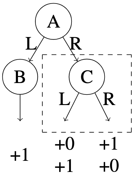
One may wonder why do pure offline RL methods fail to learn when the transfer coefficient is bounded, and why does online access help? We illustrate with the MDP construction developed by Zhan et al. [2022], Chen and Jiang [2022], visualized in Figure 2.
Consider two MDPs with , three states , two actions and the fixed start state . The two MDPs have the same dynamics but different rewards. In both, actions from state yield reward . In , yields reward while yields reward in . All other rewards are . In both and , an optimal policy is and . With where is the optimal function for , then one can easily verify that satisfies Bellman completeness, for both MDPs. Finally with offline distribution supported on states and only (with no coverage on state ), we have sufficient coverage over . However, samples from are unable to distinguish between and or ( and ), since state is not supported by . Unfortunately, adversarial tie-breaking may result the greedy policies of and visiting state , where we have no information about the correct action.
This issue has been documented before, and in order to address it with pure offline RL, existing approaches require additional structural assumptions. For instance, Chen and Jiang [2022] assume that has a gap, which usually does not hold when action space is large or continuous. Xie et al. [2021a] assumes policy-dependent Bellman completeness for every possible policy (which is much stronger than our assumption), and Zhan et al. [2022] assumes a somewhat non-interpretable realizability assumption on some “value” function that does not obey the standard Bellman equation. In contrast, by combining offline data and online data, our approach focuses on functions that have small Bellman residual under both the offline distribution and the on-policy distributions, which together with the offline data coverage assumption, ensures near optimality. It is easy to see that the hybrid approach will succeed Figure 2.
6 Experiments
In this section we discuss empirical results comparing Hy-Q to several representative RL methods on two challenging benchmarks. Our experiments focus on answering the following questions:
-
1.
Can Hy-Q efficiently solve problems that SOTA offline RL methods simply cannot?
-
2.
Can Hy-Q, via the use of offline data, significantly improve the sample efficiency of online RL?
-
3.
Does Hy-Q scale to challenging deep-RL benchmarks?
Our empirical results provide positive answers to all of these questions. To study the first two, we consider the diabolical combination lock environment [Misra et al., 2020, Zhang et al., 2022c], a synthetic environment designed to be particularly challenging for online exploration. The synthetic nature allows us to carefully control the offline data distribution to modulate the difficulty of the setup and also to compare with a provably efficient baseline [Zhang et al., 2022c]. To study the third question, we consider the Montezuma’s Revenge benchmark from the Arcade Learning environment, which is one of the most challenging empirical benchmarks with high-dimensional image inputs, largely due to the difficulties of exploration. Additional details are deferred to Appendix E.
Hy-Q implementation.
We largely follow Algorithm 1 in our implementation for the combination lock experiment. Particularly, we use a similar function approximation to Zhang et al. [2022c], and a minibatch Adam update on Eq. (1) with the same sampling proportions as in the pseudocode. For Montezuma’s Revenge, in addition to minibatch optimization, since the horizon of the environment is not fixed, we deploy a discounted version of Hy-Q. Concretely, the target value in the Bellman error is calculated from the output of a target network, which is periodically updated, times a discount factor. We refer the readers to Appendix E for more details.
Baselines.
We include representative algorithms from four categories: (1) for imitation learning we use Behavior Cloning (Bc) [Bain and Sammut, 1995], (2) for offline RL we use Conservative Q-Learning (Cql) [Kumar et al., 2020] due to its successful demonstrations on some Atari games, (3) for online RL we use Briee [Zhang et al., 2022c] for combination lock888We note that Briee is currently the state-of-the-art method for the combination lock environment. In particular, Misra et al. [2020] show that many Deep RL baselines fail in this environment. and Random Network Distillation (Rnd) [Burda et al., 2018] for Montezuma’s Revenge, and (4) as a Hybrid-RL baseline we use Deep Q-learning from Demonstrations (Dqfd) [Hester et al., 2018]. We note that Dqfd and prior hybrid RL methods combine expert demonstrations with online interactions, but are not necessarily designed to work with general offline datasets.
Results summary.
Overall, we find that Hy-Q performs favorably against all of these baselines. Compared with offline RL, imitation learning, and prior hybrid methods, Hy-Q is significantly more robust in the presence of a low quality offline data distribution. Compared with online methods, Hy-Q offers order-of-magnitude savings in the total experience.
Reproducibility.
We release our code at https://github.com/yudasong/HyQ. We also include implementation details in Appendix E.
6.1 Combination Lock
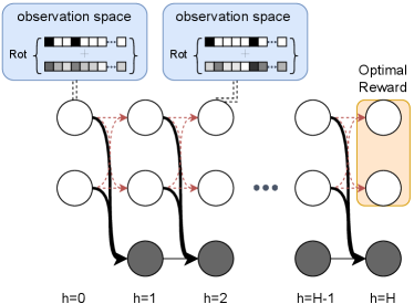
The combination lock benchmark is depicted in Figure 3 and consists of horizon , three latent states for each time step and actions in each state. Each state has a single “good” action that advances down a chain of favorable latent states (white) from which optimal reward can be obtained. A single incorrect action transitions to an absorbing chain (black latent states) with suboptimal value. The agent operates on high dimensional continuous observations omitted from latent states and must use function approximation to succeed. This is an extremely challenging problem for which many Deep RL methods are known to fail [Misra et al., 2020], in part because (uniform) random exploration only has probability of obtaining the optimal reward.
On the other hand, the model has low bilinear rank, so we do have online RL algorithms that are provably sample-efficient: Briee [Zhang et al., 2022c] currently obtains state of the art sample complexity. However, its sample complexity is still quite large, and we hope that Hybrid RL can address this shortcoming. We are not aware of any experiments with offline RL methods on this benchmark.
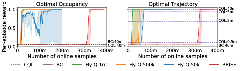
We construct two offline datasets for the experiments, both of which are derived from the optimal policy which always picks the ”good” actions and stays in the chains of white states. In the optimal trajectory dataset we collect full trajectories by following with -greedy exploration with . We also add some noise by making the agent to perform randomly at timestep . In the optimal occupancy dataset we collect transition tuples from the state-occupancy measure of with random actions.999Formally, we sample , , , , . Both datasets have bounded concentrability coefficients (and hence transfer coefficients) with respect to , but the second dataset is much more challenging since the actions in the offline dataset do not directly provide information about , as they do in the former.
The results are presented in Figure 4. First, we observe that Hy-Q can reliably solve the task under both offline distributions with relatively low sample complexity (500k offline samples and 25m online samples). In comparison, Bc fails completely since both datasets contain random actions. Cql can solve the task using the optimal trajectory-based dataset with a sample complexity that is comparable to the combined sample size of Hy-Q. However, Cql fails on the optimal occupancy-based dataset since the actions themselves are not informative. Indeed the pessimism-inducing regularizer of Cql is constant on this dataset and so the algorithm reduces to Fqi which provably fails when the offline data does not have a global coverage (i.e., covers every state-action pair). Finally, Hy-Q can solve the task with a factor of 5-10 reduction in samples (online plus offline) when compared with Briee. This demonstrates the robustness and sample efficiency provided by hybrid RL.
6.2 Montezuma’s Revenge
To answer the third question, we turn to Montezuma’s Revenge, an extremely challenging image-based benchmark environment with sparse rewards. We follow the setup from Burda et al. [2018] and introduce stochasticity to the original dynamics: with probability 0.25 the environment executes the previous action instead of the current one. For offline datasets, we first train an “expert policy” via Rnd to achieve . We create three datasets by mixing samples from with those from a random policy: the easy dataset contains only samples from , the medium dataset mixes in a 80/20 proportion (80 from ), and the hard dataset mixes in a 50/50 proportion. Here we record full trajectories from both policies in the offline dataset, but measure the proportion using the number of transition tuples instead of trajectories. We provide 0.1 million offline samples for the hybrid methods, and 1 million samples for the offline and IL methods.
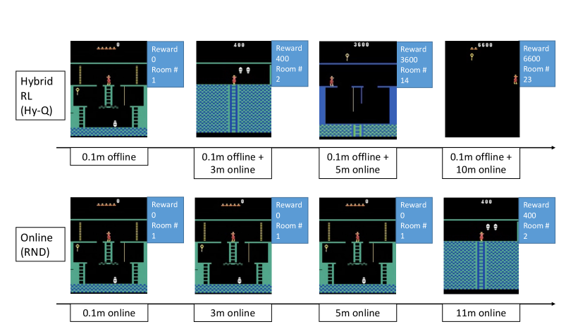
Results are displayed in Figure 5. Cql fails completely on all datasets. Dqfd performs well on the easy dataset due to the supervised learning style large margin loss [Piot et al., 2014] that imitates the policies in the offline dataset. However, Dqfd’s performance drops as the quality of the offline dataset degrades (medium), and fails when the offline dataset is low quality (hard), where one cannot simply treat offline samples as expert samples. We also observe that Bc is a competitive baseline in the first two settings due to high fraction of expert samples, and thus we view these problems as relatively easy to solve. Hy-Q is the only method that performs well on the hard dataset. Note that here, BC’s performance is quite poor. We also include the comparison with Rnd in Figure 1 and Figure 6: with only 100k offline samples from any of the three datasets, Hy-Q is over 10x more efficient in terms of online sample complexity.
7 Conclusion
We demonstrate the potential of hybrid RL with Hy-Q, a simple, theoretically principled, and empirically effective algorithm. Our theoretical results showcase how Hy-Q circumvents the computational issues of pure offline or online RL, while our empirical results highlight its robustness and sample efficiency. Yet, Hy-Q is perhaps the most natural hybrid algorithm, and we are optimistic that there is much more potential to unlock from the hybrid setting. We look forward to studying this in the future.
Acknowledgement
AS thanks Karthik Sridharan for useful discussions. WS acknowledges funding support from NSF IIS-2154711. We thank Simon Zhai for their careful reading of the manuscript and improvement on the technical correctness of our paper. We also thank Uri Sherman for their discussion on the computational efficiency of the original draft.
References
- Abbasi-Yadkori et al. [2019] Yasin Abbasi-Yadkori, Peter Bartlett, Kush Bhatia, Nevena Lazic, Csaba Szepesvari, and Gellért Weisz. Politex: Regret bounds for policy iteration using expert prediction. In International Conference on Machine Learning, 2019.
- Agarwal et al. [2019] Alekh Agarwal, Nan Jiang, Sham M Kakade, and Wen Sun. Reinforcement learning: Theory and algorithms. 2019. URL https://rltheorybook.github.io/.
- Agarwal et al. [2020a] Alekh Agarwal, Sham Kakade, Akshay Krishnamurthy, and Wen Sun. Flambe: Structural complexity and representation learning of low rank MDPs. In Advances in Neural Information Processing Systems, 2020a.
- Agarwal et al. [2020b] Alekh Agarwal, Sham M Kakade, Jason D Lee, and Gaurav Mahajan. Optimality and approximation with policy gradient methods in markov decision processes. In Conference on Learning Theory, 2020b.
- Badia et al. [2020] Adrià Puigdomènech Badia, Bilal Piot, Steven Kapturowski, Pablo Sprechmann, Alex Vitvitskyi, Zhaohan Daniel Guo, and Charles Blundell. Agent57: Outperforming the Atari human benchmark. In International Conference on Machine Learning, 2020.
- Bagnell et al. [2003] James Bagnell, Sham M Kakade, Jeff Schneider, and Andrew Ng. Policy search by dynamic programming. Advances in Neural Information Processing Systems, 2003.
- Bain and Sammut [1995] Michael Bain and Claude Sammut. A framework for behavioural cloning. In Machine Intelligence 15, 1995.
- Bellemare et al. [2013] Marc G Bellemare, Yavar Naddaf, Joel Veness, and Michael Bowling. The arcade learning environment: An evaluation platform for general agents. Journal of Artificial Intelligence Research, 2013.
- Beygelzimer et al. [2011] Alina Beygelzimer, John Langford, Lihong Li, Lev Reyzin, and Robert Schapire. Contextual bandit algorithms with supervised learning guarantees. In International Conference on Artificial Intelligence and Statistics, 2011.
- Bubeck et al. [2015] Sébastien Bubeck et al. Convex optimization: Algorithms and complexity. Foundations and Trends® in Machine Learning, 2015.
- Burda et al. [2018] Yuri Burda, Harrison Edwards, Amos Storkey, and Oleg Klimov. Exploration by random network distillation. In International Conference on Learning Representations, 2018.
- Chang et al. [2021] Jonathan Chang, Masatoshi Uehara, Dhruv Sreenivas, Rahul Kidambi, and Wen Sun. Mitigating covariate shift in imitation learning via offline data with partial coverage. Advances in Neural Information Processing Systems, 2021.
- Chen and Jiang [2019] Jinglin Chen and Nan Jiang. Information-theoretic considerations in batch reinforcement learning. In International Conference on Machine Learning, 2019.
- Chen and Jiang [2022] Jinglin Chen and Nan Jiang. Offline reinforcement learning under value and density-ratio realizability: the power of gaps. arXiv:2203.13935, 2022.
- Dani et al. [2008] Varsha Dani, Thomas P Hayes, and Sham M Kakade. Stochastic linear optimization under bandit feedback. 2008.
- Dann et al. [2022] Chris Dann, Yishay Mansour, Mehryar Mohri, Ayush Sekhari, and Karthik Sridharan. Guarantees for epsilon-greedy reinforcement learning with function approximation. In International Conference on Machine Learning, pages 4666–4689. PMLR, 2022.
- Dann et al. [2018] Christoph Dann, Nan Jiang, Akshay Krishnamurthy, Alekh Agarwal, John Langford, and Robert E Schapire. On oracle-efficient PAC RL with rich observations. In Advances in Neural Information Processing Systems, 2018.
- Du et al. [2021] Simon Du, Sham Kakade, Jason Lee, Shachar Lovett, Gaurav Mahajan, Wen Sun, and Ruosong Wang. Bilinear classes: A structural framework for provable generalization in RL. In International Conference on Machine Learning, 2021.
- Foster et al. [2021] Dylan J Foster, Akshay Krishnamurthy, David Simchi-Levi, and Yunzong Xu. Offline reinforcement learning: Fundamental barriers for value function approximation. In Conference on Learning Theory, 2021.
- Fujimoto and Gu [2021] Scott Fujimoto and Shixiang Shane Gu. A minimalist approach to offline reinforcement learning. In Advances in Neural Information Processing Systems, 2021.
- Guo et al. [2022] Zhaohan Daniel Guo, Shantanu Thakoor, Miruna Pîslar, Bernardo Avila Pires, Florent Altché, Corentin Tallec, Alaa Saade, Daniele Calandriello, Jean-Bastien Grill, Yunhao Tang, Michal Valko, R’emi Munos, Mohammad Gheshlaghi Azar, and Bilal Piot. BYOL-explore: Exploration by bootstrapped prediction. arXiv:2206.08332, 2022.
- Haarnoja et al. [2018] Tuomas Haarnoja, Aurick Zhou, Kristian Hartikainen, George Tucker, Sehoon Ha, Jie Tan, Vikash Kumar, Henry Zhu, Abhishek Gupta, Pieter Abbeel, and Sergey Levine. Soft actor-critic algorithms and applications. arXiv:1812.05905, 2018.
- Hester et al. [2018] Todd Hester, Matej Vecerik, Olivier Pietquin, Marc Lanctot, Tom Schaul, Bilal Piot, Dan Horgan, John Quan, Andrew Sendonaris, Ian Osband, John Agapiou, Joel Z. Leibo, and Audrunas Gruslys. Deep Q-learning from demonstrations. In AAAI Conference on Artificial Intelligence, 2018.
- Jia et al. [2022] Zhiwei Jia, Xuanlin Li, Zhan Ling, Shuang Liu, Yiran Wu, and Hao Su. Improving policy optimization with generalist-specialist learning. In International Conference on Machine Learning, pages 10104–10119. PMLR, 2022.
- Jiang and Huang [2020] Nan Jiang and Jiawei Huang. Minimax value interval for off-policy evaluation and policy optimization. Advances in Neural Information Processing Systems, 2020.
- Jiang et al. [2017] Nan Jiang, Akshay Krishnamurthy, Alekh Agarwal, John Langford, and Robert E Schapire. Contextual decision processes with low Bellman rank are PAC-learnable. In International Conference on Machine Learning, 2017.
- Jin et al. [2020] Chi Jin, Zhuoran Yang, Zhaoran Wang, and Michael I Jordan. Provably efficient reinforcement learning with linear function approximation. In Conference on Learning Theory, 2020.
- Jin et al. [2021a] Chi Jin, Qinghua Liu, and Sobhan Miryoosefi. Bellman eluder dimension: New rich classes of RL problems, and sample-efficient algorithms. Advances in Neural Information Processing Systems, 2021a.
- Jin et al. [2021b] Ying Jin, Zhuoran Yang, and Zhaoran Wang. Is pessimism provably efficient for offline RL? In International Conference on Machine Learning, 2021b.
- Kakade [2001] Sham M Kakade. A natural policy gradient. Advances in Neural Information Processing Systems, 2001.
- Kakade and Langford [2002] Sham M Kakade and John Langford. Approximately optimal approximate reinforcement learning. In International Conference on Machine Learning, 2002.
- Kalashnikov et al. [2018] Dmitry Kalashnikov, Alex Irpan, Peter Pastor, Julian Ibarz, Alexander Herzog, Eric Jang, Deirdre Quillen, Ethan Holly, Mrinal Kalakrishnan, Vincent Vanhoucke, et al. Qt-opt: Scalable deep reinforcement learning for vision-based robotic manipulation. arXiv preprint arXiv:1806.10293, 2018.
- Kane et al. [2022] Daniel Kane, Sihan Liu, Shachar Lovett, and Gaurav Mahajan. Computational-statistical gaps in reinforcement learning. In Conference on Learning Theory, 2022.
- Kostrikov et al. [2021] Ilya Kostrikov, Ashvin Nair, and Sergey Levine. Offline reinforcement learning with implicit Q-learning. arXiv:2110.06169, 2021.
- Kumar et al. [2020] Aviral Kumar, Aurick Zhou, George Tucker, and Sergey Levine. Conservative Q-learning for offline reinforcement learning. In Advances in Neural Information Processing Systems, 2020.
- Lattimore and Szepesvári [2020] Tor Lattimore and Csaba Szepesvári. Bandit algorithms. Cambridge University Press, 2020.
- Lee et al. [2022] Seunghyun Lee, Younggyo Seo, Kimin Lee, Pieter Abbeel, and Jinwoo Shin. Offline-to-online reinforcement learning via balanced replay and pessimistic q-ensemble. In Conference on Robot Learning, pages 1702–1712. PMLR, 2022.
- Levine et al. [2020] Sergey Levine, Aviral Kumar, George Tucker, and Justin Fu. Offline reinforcement learning: Tutorial, review, and perspectives on open problems. arXiv:2005.01643, 2020.
- Lillicrap et al. [2016] Timothy P Lillicrap, Jonathan J Hunt, Alexander Pritzel, Nicolas Heess, Tom Erez, Yuval Tassa, David Silver, and Daan Wierstra. Continuous control with deep reinforcement learning. In International Conference on Learning Representations, 2016.
- Liu and Brunskill [2018] Yao Liu and Emma Brunskill. When simple exploration is sample efficient: Identifying sufficient conditions for random exploration to yield pac rl algorithms. arXiv preprint arXiv:1805.09045, 2018.
- Misra et al. [2020] Dipendra Misra, Mikael Henaff, Akshay Krishnamurthy, and John Langford. Kinematic state abstraction and provably efficient rich-observation reinforcement learning. In International conference on machine learning, 2020.
- Mnih et al. [2015] Volodymyr Mnih, Koray Kavukcuoglu, David Silver, Andrei A Rusu, Joel Veness, Marc G Bellemare, Alex Graves, Martin Riedmiller, Andreas K Fidjeland, Georg Ostrovski, Stig Petersen, Charles Beattie, Amir Sadik, Ioannis Antonoglou, Helen King, Dharshan Kumaran, Daan Wierstra, Shane Legg, and Demis Hassabis. Human-level control through deep reinforcement learning. Nature, 2015.
- Modi et al. [2021] Aditya Modi, Jinglin Chen, Akshay Krishnamurthy, Nan Jiang, and Alekh Agarwal. Model-free representation learning and exploration in low-rank MDPs. arXiv:2102.07035, 2021.
- Munos and Szepesvári [2008] Rémi Munos and Csaba Szepesvári. Finite-time bounds for fitted value iteration. Journal of Machine Learning Research, 2008.
- Nair et al. [2018] Ashvin Nair, Bob McGrew, Marcin Andrychowicz, Wojciech Zaremba, and Pieter Abbeel. Overcoming exploration in reinforcement learning with demonstrations. In IEEE International Conference on Robotics and Automation, 2018.
- Nair et al. [2020] Ashvin Nair, Murtaza Dalal, Abhishek Gupta, and Sergey Levine. Accelerating online reinforcement learning with offline datasets. arXiv:2006.09359, 2020.
- Niu et al. [2022] Haoyi Niu, Shubham Sharma, Yiwen Qiu, Ming Li, Guyue Zhou, Jianming Hu, and Xianyuan Zhan. When to trust your simulator: Dynamics-aware hybrid offline-and-online reinforcement learning. arXiv preprint arXiv:2206.13464, 2022.
- Piot et al. [2014] Bilal Piot, Matthieu Geist, and Olivier Pietquin. Boosted bellman residual minimization handling expert demonstrations. In Joint European Conference on Machine Learning and Knowledge Discovery in Databases, 2014.
- Qiu et al. [2022] Shuang Qiu, Lingxiao Wang, Chenjia Bai, Zhuoran Yang, and Zhaoran Wang. Contrastive UCB: Provably efficient contrastive self-supervised learning in online reinforcement learning. In International Conference on Machine Learning, 2022.
- Rajeswaran et al. [2017] Aravind Rajeswaran, Vikash Kumar, Abhishek Gupta, Giulia Vezzani, John Schulman, Emanuel Todorov, and Sergey Levine. Learning complex dexterous manipulation with deep reinforcement learning and demonstrations. arXiv:1709.10087, 2017.
- Ross and Bagnell [2012] Stephane Ross and J Andrew Bagnell. Agnostic system identification for model-based reinforcement learning. arXiv:1203.1007, 2012.
- Schaul et al. [2015] Tom Schaul, John Quan, Ioannis Antonoglou, and David Silver. Prioritized experience replay. arXiv:1511.05952, 2015.
- Schrittwieser et al. [2020] Julian Schrittwieser, Ioannis Antonoglou, Thomas Hubert, Karen Simonyan, Laurent Sifre, Simon Schmitt, Arthur Guez, Edward Lockhart, Demis Hassabis, Thore Graepel, Timothy Lillicrap, and David Silver. Mastering Atari, Go, chess and Shogi by planning with a learned model. Nature, 2020.
- Schulman et al. [2015] John Schulman, Sergey Levine, Pieter Abbeel, Michael Jordan, and Philipp Moritz. Trust region policy optimization. In International Conference on Machine Learning, 2015.
- Schulman et al. [2017] John Schulman, Filip Wolski, Prafulla Dhariwal, Alec Radford, and Oleg Klimov. Proximal policy optimization algorithms. arXiv:1707.06347, 2017.
- Sekhari et al. [2021] Ayush Sekhari, Christoph Dann, Mehryar Mohri, Yishay Mansour, and Karthik Sridharan. Agnostic reinforcement learning with low-rank MDPs and rich observations. Advances in Neural Information Processing Systems, 2021.
- Shalev-Shwartz and Ben-David [2014] Shai Shalev-Shwartz and Shai Ben-David. Understanding machine learning: From theory to algorithms. Cambridge University Press, 2014.
- Sun et al. [2019] Wen Sun, Nan Jiang, Akshay Krishnamurthy, Alekh Agarwal, and John Langford. Model-based RL in contextual decision processes: PAC bounds and exponential improvements over model-free approaches. In Conference on learning theory, 2019.
- Uchendu et al. [2022] Ikechukwu Uchendu, Ted Xiao, Yao Lu, Banghua Zhu, Mengyuan Yan, Joséphine Simon, Matthew Bennice, Chuyuan Fu, Cong Ma, Jiantao Jiao, Sergey Levine, and Karol Hausman. Jump-start reinforcement learning. arXiv:2204.02372, 2022.
- Uehara and Sun [2021] Masatoshi Uehara and Wen Sun. Pessimistic model-based offline reinforcement learning under partial coverage. In International Conference on Learning Representations, 2021.
- Uehara et al. [2021] Masatoshi Uehara, Xuezhou Zhang, and Wen Sun. Representation learning for online and offline RL in low-rank MDPs. arXiv:2110.04652, 2021.
- Van Hasselt et al. [2016] Hado Van Hasselt, Arthur Guez, and David Silver. Deep reinforcement learning with double Q-learning. In AAAI Conference on Artificial Intelligence, 2016.
- Vecerik et al. [2017] Mel Vecerik, Todd Hester, Jonathan Scholz, Fumin Wang, Olivier Pietquin, Bilal Piot, Nicolas Heess, Thomas Rothörl, Thomas Lampe, and Martin Riedmiller. Leveraging demonstrations for deep reinforcement learning on robotics problems with sparse rewards. arXiv:1707.08817, 2017.
- Wang et al. [2021] Ruosong Wang, Yifan Wu, Ruslan Salakhutdinov, and Sham Kakade. Instabilities of offline rl with pre-trained neural representation. In International Conference on Machine Learning, 2021.
- Wang et al. [2016] Ziyu Wang, Tom Schaul, Matteo Hessel, Hado Hasselt, Marc Lanctot, and Nando Freitas. Dueling network architectures for deep reinforcement learning. In International Conference on Machine Learning, 2016.
- Xie and Jiang [2021] Tengyang Xie and Nan Jiang. Batch value-function approximation with only realizability. In International Conference on Machine Learning, 2021.
- Xie et al. [2021a] Tengyang Xie, Ching-An Cheng, Nan Jiang, Paul Mineiro, and Alekh Agarwal. Bellman-consistent pessimism for offline reinforcement learning. Advances in Neural Information Processing Systems, 2021a.
- Xie et al. [2021b] Tengyang Xie, Nan Jiang, Huan Wang, Caiming Xiong, and Yu Bai. Policy finetuning: Bridging sample-efficient offline and online reinforcement learning. Advances in Neural Information Processing Systems, 2021b.
- Yang and Wang [2019] Lin Yang and Mengdi Wang. Sample-optimal parametric Q-learning using linearly additive features. In International Conference on Machine Learning, 2019.
- Yu et al. [2021] Tianhe Yu, Aviral Kumar, Rafael Rafailov, Aravind Rajeswaran, Sergey Levine, and Chelsea Finn. Combo: Conservative offline model-based policy optimization. In Advances in Neural Information Processing Systems, 2021.
- Zanette et al. [2020] Andrea Zanette, Alessandro Lazaric, Mykel Kochenderfer, and Emma Brunskill. Learning near optimal policies with low inherent Bellman error. In International Conference on Machine Learning, 2020.
- Zanette et al. [2021] Andrea Zanette, Martin J Wainwright, and Emma Brunskill. Provable benefits of actor-critic methods for offline reinforcement learning. Advances in Neural Information Processing Systems, 2021.
- Zhan et al. [2022] Wenhao Zhan, Baihe Huang, Audrey Huang, Nan Jiang, and Jason Lee. Offline reinforcement learning with realizability and single-policy concentrability. In Conference on Learning Theory, pages 2730–2775. PMLR, 2022.
- Zhang et al. [2022a] Tianjun Zhang, Tongzheng Ren, Mengjiao Yang, Joseph Gonzalez, Dale Schuurmans, and Bo Dai. Making linear MDPs practical via contrastive representation learning. In International Conference on Machine Learning, 2022a.
- Zhang et al. [2022b] Xuezhou Zhang, Yiding Chen, Xiaojin Zhu, and Wen Sun. Corruption-robust offline reinforcement learning. In International Conference on Artificial Intelligence and Statistics, 2022b.
- Zhang et al. [2022c] Xuezhou Zhang, Yuda Song, Masatoshi Uehara, Mengdi Wang, Alekh Agarwal, and Wen Sun. Efficient reinforcement learning in block MDPs: A model-free representation learning approach. In International Conference on Machine Learning, 2022c.
Appendix A Proofs for Section 5
Additional notation.
Throughout the appendix, we define the feature covariance matrix as
| (3) |
Furthermore, given a distribution and a function , we denote its weighted norm as .
A.1 Supporting lemmas for Theorem 1
Before proving Theorem 1, we first present a few useful lemma. We start with a standard result on least square generalization bound, which is be used by recalling that Algorithm 1 performs least squares on the empirical bellman error. We defer the proof of Lemma 3 to Appendix B.
Lemma 3.
(Least squares generalization bound) Let , , we consider a sequential function estimation setting, with an instance space and target space . Let be a class of real valued functions. Let be a dataset of points where , and is sampled via the conditional probability :
where the function satisfies approximate realizability i.e.
and are independent random variables such that . Additionally, suppose that and . Then the least square solution satisfies with probability at least ,
The above lemma is basically an extension of the standard least square regression agnostic generalization bound from i.i.d. setting to the non-i.i.d. case with the sequence of training data forms a sequence of Martingales. We state the result when the realizability only holds approximately upto the approximation . However, for all our proofs, we invoke this result by setting .
In the next two lemmas, we prove two lemmas where we can bound each part of the regret decomposition using the Bellman error of the value function .
Lemma 4 (Performance difference lemma).
For any function where and , we have
where we define for all .
Proof.
We start the proof by noting that , then we have:
| (4) |
Then by recursively applying the same procedure on the second term in (4), we have
Finally for , we recall that we set and for notation simplicity. Thus we have:
∎
Now we proceed to how to bound the other half in the regret decomposition:
Lemma 5.
Let be a comparator policy, and consider any value function where . Then,
where we defined for all .
Proof.
The following result is useful in the bilinear models when we want to bound the potential functions. The result directly follows from the elliptical potential lemma [Lattimore and Szepesvári, 2020, Lemma 19.4].
Lemma 6.
Let be a sequence of vectors with for all . Then,
where the matrix for and , and the matrix norm .
Proof.
Since , we have that
Thus, using elliptical potential lemma [Lattimore and Szepesvári, 2020, Lemma 19.4], we get that
The desired bound follows from Jensen’s inequality which implies that
∎
A.2 Proof of Theorem 1
Before delving into the proof, we first state that following generalization bound for FQI.
Lemma 7 (Bellman error bound for FQI).
Let and let for and , be the estimated value function for time step computed via least square regression using samples in the dataset in (1) in the iteration of Algorithm 1. Then, with probability at least , for any and ,
| and | |||
where denotes the offline data distribution at time , and the distribution is defined such that .
Proof.
Fix , and and consider the regression problem ((1) in the iteration of Algorithm 1):
which can be thought of as regression problem
where dataset consisting of samples where
In particular, we define such that the first samples , the next samples , and so on where the samples . Note that: (a) for any sample in , we have that
where the last line holds since the Bellman completeness assumption implies existence of such a function , (b) for any sample, and for all , (c) our construction of implies that for each iteration , the sample are generated in the following procedure: is sampled from the data generation scheme , and is sampled from some conditional probability distribution as defined in Lemma 3, finally (d) the samples in are drawn from the offline distribution , and the samples in are drawn such that and . Thus, using Lemma 3, we get that the least square regression solution satisfies
Using the property-(d) in the above, we get that
where the distribution is defined by sampling and . Taking a union bound over and , and bounding each term separately, gives the desired statement. ∎
We next note a change in distribution lemma which allows us to bound expected bellman error under the distribution generated by in terms of the expected square bellman error w.r.t. the previous policies data distribution, which is further controlled using regression.
Lemma 8.
Proof.
Using Cauchy-Schwarz inequality, we get that
| (6) | ||||
where the inequality in the second last line holds by plugging in the bound on , and the last line holds by using Definition 2 which implies that
where the last inequality is due to Jensen’s inequality. ∎
We now have all the tools to prove Theorem 1. We first restate the bound with the exact problem dependent parameters, assumign that and are constants which are hidden in the order notation below.
Theorem (Theorem 1 restated).
Let and . Then, with probability at least , the cumulative suboptimality of Algorithm 1 is bounded as
Proof of Theorem 1.
Let be any comparator policy with bounded transfer coefficient i.e.
| (7) |
We start by noting that
| (8) |
For the first term in the right hand side of (8), note that using Lemma 5 for each for , we get
| (9) |
where the second inequality follows from plugging in the definition of in (7). The last line follows from Lemma 7.
For the second term in (8), using Lemma 4 for each for , we get
| (10) | ||||
where the second line follows from Definition 2, the third line follows from Lemma 8 and by plugging in the bound in Lemma 7. Using the bound in Lemma 6 in the above, we get that
| (11) |
where the second line follows by plugging in .
Plugging in the values of and in the above, and using subadditivity of square-root, we get that
Setting and in the above gives the cumulative suboptimality bound
| (12) |
∎
Proof of Corollary 1.
We next convert the above cumulative suboptimality bound into sample complexity bound via a standard online-to-batch conversion. Setting in (12) and defining the policy , we get that
Thus, we get that for , we get that
In these iterations, the total number of offline samples used is
and the total number of online samples used is
where the additional factor appears because we collect samples for every in the algorithm. ∎
A.3 V-type Bilinear Rank
Our previous result focus on the Q-type bilinear model. Here we provide the V-type Bilinear rank definition. This V-type Bilinear rank definition is basically the same as the low Bellman rank model proposed by Jiang et al. [2017].
Definition 5 (V-type Bilinear model).
Consider any pair of functions with . Denote the greedy policy of as . We say that the MDP together with the function admits a bilinear structure of rank if for any , there exist two (unknown) mappings and with and , such that:
Note that different from the Q-type definition, here the action is taken from the greedy policy with respect to . This way can serve as an approximation of – thus the name of -type.
To make Hy-Q work for the V-type Bilinear model, we only need to make slight change on the data collection process, i.e., when we collect online batch , we sample . Namely the action is taken uniformly randomly here. We provide the pseudocode in Algorithm 2. We refer the reader to Du et al. [2021], Jin et al. [2021a] for a detailed discussion.
| (13) |
A.3.1 Complexity bound for V-type Bilinear models
In this section, we give a performance analysis of Algorithm 2 for V-type Bilinear models. The contents in this section extend the results developed for Q-type Bilinear models in Section A.2 to V-type Bilinear models.
We first note the following bound for FQI estimates in Algorithm 2.
Lemma 9.
Let and let for and , be the estimated value function for time step computed via least square regression using samples in the dataset in (13) in the iteration of Algorithm 2. Then, with probability at least , for any and ,
| and | |||
where denotes the offline data distribution at time , and the distribution is defined such that and .
The following change in distribution lemma is the version of Lemma 8 under V-type Bellman rank assumption.
Lemma 10.
Suppose the underlying model is a V-type bilinear model. Then, for any and , we have
where is defined in (3).
Proof.
The proof is identical to the proof of Lemma 8. Repeating the analysis till (6), we get that
where the second line above follows from the definition of V-type bilinear model in Definition 5, and the last line holds because:
where the first inequality above is due to Jensen’s inequality and the last inequality follows form a straightforward upper bound since each term inside the expectation is non-negative. ∎
We are finally ready to state and prove our main result in this section.
Theorem 2 (Cumulative suboptimality bound for V-type bilinear rank models).
Let and . Then, with probability at least , the cumulative suboptimality of Algorithm 2 is bounded as
Proof.
The proof follows closely the proof of Theorem 1. Repeating the analysis till (8) and (9), we get that:
| (14) |
For the second term in the above, using Lemma 4 for each for , we get
where the second line follows from Definition 5, and the last line follows from Lemma 10 and by plugging in the bound in Lemma 9. Using the elliptical potential Lemma 6 as in the proof of Theorem 1, we get that
Plugging in the values of and from Lemma 9 in the above, and using subadditivity of square-root, we get that
Setting and , we get the following cumulative suboptimality bound:
| (15) |
∎
Corollary 2 (Sample complexity).
Under the assumptions of Theorem 2 if then Algorithm 2 can find an -suboptimal policy for which with total sample complexity of:
Proof.
The following follows from a standard online-to-batch conversion. Setting in (15) and defining the policy , we get that
Thus, we the policy returned after satisfies In these iterations, the total number of offline samples used is
and the total number of online samples collected is
where the additional factor appears because we collect samples for every in the algorithm. ∎
A.4 Bounds on transfer coefficient
Note that takes both the distribution shift and the function class into consideration, and is smaller than the existing density ratio based concentrability coefficient [Kakade and Langford, 2002, Munos and Szepesvári, 2008, Chen and Jiang, 2019] and also existing Bellman error based concentrability coefficient Xie et al. [2021a]. We formalize this in the following lemma.
Lemma 11.
For any and offline distribution ,
Proof.
Using Jensen’s inequality, we get that
where the second line follows from the Mediant inequality and the last line holds whenever . ∎
Next we show that in the linear Bellman complete setting, is bounded by the relative condition number using the linear features.
Lemma 12.
Consider the linear Bellman complete setting (Definition 3) with known feature . Suppose that the feature covariance matrix induced by offline distribution : is invertible. Then for any policy , we have
Proof.
Repeating the argument in Lemma 11, we have
Recall that in linear Bellman complete setting, we can write as , and for any that defines , there exists such that . ∎
Now we proceed to low-rank MDPs where feature is unknown. We show that for low-rank MDPs, is bounded by the partial feature coverage using the unknown ground truth feature.
Lemma 13.
Consider the low-rank MDP setting (Definition 4) where the transition dynamics is given by for some . Suppose that the offline distribution is such that for any . Furthermore, suppose that is induced via trajectories i.e. and for any , and that the feature covariance matrix is invertible.101010This is for notation simplicity, and we emphasize that we do not assume eigenvalues are lower bounded. In other words, eigenvalue of this feature covariance matrix could approach to . Then for any policy , we have
Proof.
We first upper bound the numerator separately. First note that for ,
| (16) |
where the last inequality follows from our assumption since .
Next, for any , we note that backing up one step and looking at the pair that lead to the state , we get that
| (17) |
where the last line follows from an application of Cauchy-Schwarz inequality. For the term inside the expectation in the right hand side above, we note that,
| (18) |
where follows by expanding the norm , follows an application of Jensen’s inequality, is due to our assumption that the offline dataset is generated using trajectories such that . Finally, follows from the definition of . Plugging (18) in (17), we get that for ,
| (19) |
We are now ready to bound the transfer coefficient. First note that using (16), for any ,
Furthermore, for any , using (19), we get that
where the last line holds for an appropriate choice of (e.g. ). Combining the above two bounds in the definition of we get that
∎
Note that in the above result, the transfer coefficient is upper bounded by the relative coverage under unknown feature and a term related to the action coverage, i.e., . This matches to the coverage condition used in prior offline RL works for low-rank MDPs [Uehara and Sun, 2021].
Appendix B Auxiliary Lemmas
In this section, we provide a few results and their proofs that we used in the previous sections. We first with the following form of Freedman’s inequality that is a modification of a similar inequality in [Beygelzimer et al., 2011].
Lemma 14 (Freedman’s Inequality).
Let be a sequence of non-negative random variables where each is sampled from some process that depends on all previous instances, i.e, . Further, suppose that almost surely for all . Then, for any and , with probability at least ,
Proof.
Define the random variable . Clearly, is a martingale difference sequence. Furthermore, we have that for any , and that
| (20) |
where the last inequality holds because .
Next we give a formal proof of Lemma 3, which gives a generalization bound for least squares regression when the samples are adapted to an increasing filtration (and are not necessarily i.i.d.). The proof follows similarly to Agarwal et al. [2019, Lemma A.11].
Lemma 15 (Lemma 3 restated: Least squares generalization bound).
Let , , we consider a sequential function estimation setting, with an instance space and target space . Let be a class of real valued functions. Let be a dataset of points where , and is sampled via the conditional probability :
where the function satisfies approximate realizability i.e.
and are independent random variables such that . Additionally, suppose that and . Then the least square solution satisfies with probability at least ,
Proof.
Consider any fixed function and define the random variable
Define the notation to denote , and note that
| (21) |
where the last line holds because . Furthermore, we also have that
| (22) |
Now we can note that the sequence of random variables satisfies the condition in Lemma 14 with. Thus we get that for any and , with probability at least ,
where the last inequality uses (21) and (22). Setting in the above, and taking a union bound over , we get that for any and , with probability at least ,
Rearranging the terms and using (21) in the above implies that,
| and | |||
| (23) | |||
For the rest of the proof, we condition on the event that (23) holds for all .
Define the function . Using (23), we get that
where the last inequality follows from the approximate realizability assumption. Let denote the least squares solution on dataset . By definition, we have that
Combining the above two relations, we get that
| (24) |
Appendix C Low Bellman Eluder Dimension problems
In this section, we consider problems with low Bellman Eluder dimensions Jin et al. [2021a]. This complexity measure is a distributional version of the Eluder dimension applied to the class of Bellman residuals w.r.t. . We show that our algorithm Hy-Q gives a similar performance guarantee for problems with small Bellman Eluder dimensions. This demonstrates that Hy-Q applies to any general model-free RL frameworks known in the RL literature so far.
We first introduce the key definitions:
Definition 6 (-independence between distributions [Jin et al., 2021a]).
Let be a class of functions defined on a space , and be probability measures over . We say is -independent of with respect to if there exists such that , but .
Definition 7 (Distributional Eluder (DE) dimension).
Let be a function class defined on , and be a family of probability measures over . The distributional Eluder dimension is the length of the longest sequence such that there exists where is -independent of for all .
Definition 8 (Bellman Eluder (BE) dimension [Jin et al., 2021a]).
Given a value function class , let be the set of Bellman residuals induced by at step , and be a collection of probability measure families over . The -Bellman Eluder dimension of with respect to is defined as
We also note the following lemma that controls the rate at which Bellman error accumulates.
Lemma 16 (Lemma 41, [Jin et al., 2021a]).
Given a function class defined on a space with , and a set of probability measures over . Suppose that the sequence and satisfy that for all . Then, for all and ,
We next state our main theorem whose proof is similar to that of Theorem 1.
Theorem 3 (Cumulative suboptimality).
Fix , and , and suppose that the underlying MDP admits Bellman eluder dimention , and the function class satisfies Assumption 1. Then with probability at least , Algorithm 1 obtains the following bound on cumulative subpotimality w.r.t. any comparator policy ,
where is the greedy policy w.r.t. at round and . Here is the class of occupancy measures that can be be induced by greedy policies w.r.t. value functions in .
Proof.
Using the bound in Lemma 7 and Lemma 16 in the above, we get that
where denotes the set of Bellman residuals induced by at step , and is the collection of occupancy measures at step induced by greedy policies w.r.t. value functions in . We set and define . Ignoring the lower order terms, we get that
where hides lower order terms, multiplying constants and log factors. Setting and , we get that
∎
Appendix D Comparison with previous works
As mentioned in the main text, many previous empirical works consider combining offline expert demonstrations with online interaction [Rajeswaran et al., 2017, Hester et al., 2018, Nair et al., 2018, 2020, Vecerik et al., 2017, Lee et al., 2022, Jia et al., 2022, Niu et al., 2022]. Thus the idea of performing RL algorithm on both offline data (expert demonstrations) and online data is also explored in some of the previous works, for example, Vecerik et al. [2017] runs DDPG on both the online and expert data, and Hester et al. [2018] uses DQN on both data but with an additional supervised loss. Since we already compared with Hester et al. [2018] in the experiment, here we focus on our discussion with Vecerik et al. [2017].
We first emphasize that Vecerik et al. [2017] only focuses on expert demonstrations and their experiments entirely rely on using expert demonstrations, while we focus on more general offline dataset that is not necessarily coming from experts. Said though, the DDPG-based algorithm from Vecerik et al. [2017] potentially can be used when offline data is not from experts. Although the algorithm from Vecerik et al. [2017] and Hy-Q share the same high-level intuition that one should perform RL on both the datasets, there are still a few differences : (1) Hy-Q uses Q-learning instead of deterministic policy gradients; note that deterministic policy gradient methods cannot be directly applied to discrete action setting; (2) Hy-Q does not require n-step TD style update, since in off-policy case, without proper importance weighting, n-step TD could incur strong bias. While proper tuning on n could balance bias and variance, one does not need to tune such n-step at all in Hy-Q; (3) The idea of keeping a non-zero ratio to sample offline dataset is also proposed in Vecerik et al. [2017]. Our buffer ratio is derived from our theory analysis but meanwhile proves the advantage of the similar heuristic applied in Vecerik et al. [2017]. (4) In their experiment, Vecerik et al. [2017] only considers expert demonstrations. In our experiment, we considered offline datasets with different amounts of transitions from very low-quality policies and showed Hy-Q is robust to low-quality transitions in offline data. Note that some of the differences may seem minor on the implementation level, but they may be important to the theory.
Regarding the experiments, our experimental evaluation adds the following insights over those in Vecerik et al. [2017]: (i) hybrid methods can succeed without expert data, (ii) hybrid methods can succeed in hard exploration discrete-action tasks, (iii) the core algorithm (-learning vs DDPG) is not essential although some details may matter. Due to the similarity between the two methods, we believe some of these insights may also translate to Vecerik et al. [2017] and we expect that the choice between Hy-Q and Hy-DDPG will be environment specific, as it is with the purely online versions of these methods. In some situations, -learning works does not immediately imply Deterministic policy gradient methods work, nor vice versa. Nevertheless, it is beyond the scope of this paper to rigorously verify this claim and we deem the study of Actor-critic algorithms in Hybrid RL setting an interesting future direction.
Appendix E Experiment Details
E.1 Combination Lock
In this section we provide a detailed description of combination lock experiment. The combination lock environment has a horizon and 10 actions at each state. There are three latent states for each timestep , where are good states and is the bad state. For each good state, we randomly pick a good action , such that in latent state , taking the good action will result in 0.5 probability of transiting to and 0.5 probability of transiting to while taking all other actions will result in a 1 probability of transiting to . At , all actions will result in a deterministic transition to . For the reward, we give an optimal reward of 1 for landing . We also give an anti-shaped reward of 0.1 for all transitions from a good state to a bad state. All other transitions have a reward of 0. The initial distribution is a uniform distribution over and . The observation space has dimension , created by concatenating a one-hot representation of the latent state and a one-hot representation of the horizon (appending 0 if necessary). Random noise from is added to each dimension, and finally the observation is multiplied by a Hadamard matrix. Note that in this environment, the agent needs to perform optimally for all timesteps to hit the final good state for an optimal reward of 1. Once the agent chooses a bad action, it will stay in the bad state until the end with at most 0.1 possible reward for the trajectory received while transitting from a good state to a bad state.
E.2 Implementation Details of Combination Lock experiment
We train separate Q-functions for all timesteps. Our function class consists of an encoder and a decoder. For the encoder, we feed the observation into one linear layer with 3 outputs, followed by a softmax layer to get a state-representation. This design of encoder is intended to learn a one-hot representation of the latent state. We take a Kronecker Product of the state-representation and the action, and feed the result to a linear layer with only one output, which will be our Q value. In order to stabilize the training, we warm-start the Q-function of timestep with the encoder from the Q-function at timestep of the current iteration and the decoder from the Q-function at time step of the previous iteration, for each iteration of training.
One remark is that since combination lock belongs to Block MDPs, we require a V-type algorithm instead of the Q-type algorithm as shown in the main text. The only difference lies in the online sampling process: instead of sampling from , for each , we sample from , i.e., we first rollin with respect to to timestep , then take a random action, observe the transition and collect that tuple. See Algorithm 2.
For CQL, we implemented the variant of CQL-DQN and picked the peak in the learning curve to report in the main paper (so in other words, we pick the best performance of CQL using online samples). While CQL is supposed to be a pure offline RL baseline, we simply tune the hyperparameters of CQL using online samples. Thus our reported results can be regarded as an upper bound on the performance that CQL would get if it were trained in the pure offline setting.
E.3 Implementation Details of Montezuma’s Revenge experiment
For Montezuma’s Revenge, we follow the Atari game convention and use a discounted setting with discount factor being 0.99. In this section we provide the detailed algorithm for the discounted setting. The overall algorithm is described in Algorithm 3. For the function approximation, we use a class of convolutional neural networks (parameterized by class ) as promoted by the original Dqn paper [Mnih et al., 2015]. We include several standard empirical design choices that have been commonly used to stabilize the training: we use Prioritize Experience Replay [Schaul et al., 2015] for our buffer. We also add Double Dqn [Van Hasselt et al., 2016] and Dueling Dqn [Wang et al., 2016] during our Q-update. These are the standard heuristics that have been used in Q learning implementation commonly. We also observe that a decaying schedule on the offline sample ratio and the exploration rate also helps provide better performance. Note that an annealing does not contradict to our comment in Section 4 on catastrophic forgetting because always has a lower bound and indeed never decreases to zero when the online learning process proceeds. In addition, we also perform value function update very inside each episode, instead of per episode update since this has been the popular design choice and leads to better efficiency in practice.
E.4 Baseline implementation
E.4.1 Combination Lock
We use the open-sourced implementation https://github.com/BY571/CQL/tree/main/CQL-DQN for Cql. For Briee, we use the official code released by the authors: https://github.com/yudasong/briee, where we rely on the code there for the combination lock environment.
E.4.2 Montezuma’s Revenge
We use the open-sourced implementation
https://github.com/jcwleo/random-network-distillation-pytorch for Rnd. For Cql, we use https://github.com/takuseno/d3rlpy for their implementation of Cql for atari. We use https://github.com/felix-kerkhoff/DQfD for Dqfd. For all baselines, we keep the hyperparameters used in these public repositories. For Cql and Dqfd, we provide the offline datasets as described in the main text instead of using the offline dataset provided in the public repositories.111111We note that Cql also fails completely with the original offline dataset (with 1 million samples) provided in the public repository. All baselines are tested in the same stochastic environment setup as in Burda et al. [2018].
E.5 Hardware Infrastructure
We run our experiments on a cluster of computes with Nvidia RTX 3090 GPUs and various CPUs which do not incur any randomness to the results.
E.6 Hyperparameters
E.6.1 Combination Lock
We provide the hyperparameters of Hy-Q in Table. 1. In addition, we provide the hyperparameters we tried for Cql baseline in Table. 2.
| Value Considered | Final Value | |
|---|---|---|
| Learning rate | {1e-2, 2e-2, 1e-3} | 2e-2 |
| Buffer size | {1e8} | 1e8 |
| Optimizer | {Adam, SGD} | Adam |
| Number of updates per iteration | {30, 300, 500} | 500 |
| Batch size | {512} | 512 |
| Value Considered | Final Value | |
|---|---|---|
| Learning rate | {1e-3} | 1e-3 |
| Optimizer | {Adam} | Adam |
| Buffer size | {1e8} | 1e8 |
| Batch size | {512} | 512 |
| Discount Factor | {0.99} | 0.99 |
| Moving Average Factor | {0.01, 0.1, 1} | 0.01 |
| Weight on CQL loss | {0, 0.1, 0.01} | 0.1 |
E.6.2 Montezuma’s Revenge
We provide the hyperparameter of Hy-Q in Table. 3. We reuse many hyperparameter choices from Dqfd. Note that denotes a decreasing/increasing schedule from to .
| Value Considered | Final Value | |
| Learning rate | {6.25e-5, [1e-4,1e-5]} | [1e-4,1e-5] |
| Offline Schedule | {0.5,0.2,[0.2,0.01]} | [0.2,0.01] |
| Exploration rate | {[0.25,0.001]} | [0.25,0.001] |
| Minibatch size | {32} | 32 |
| Weight decay (regularization) coefficient | {1e-5} | 1e-5 |
| Gradient Clipping | {10,20} | 10 |
| Discount factor | {0.99} | 0.99 |
| Value function update frequency | {4} | 4 |
| Target function update frequency | {1000,2000,5000,10000} | 10000 |
| Buffer size | {} | |
| PER Importance Sampling ratio | {[0.6,1]} | [0.6,1] |
| Online PER | {0.001} | 0.001 |
| Offline PER | {0.0001} | 0.0001 |
| Online PER Priority Coefficient | {0.4} | 0.4 |
| Offline PER Priority Coefficient | {1} | 1 |