Hybrid Spatial-Temporal Entropy Modelling for
Neural Video Compression
Abstract.
For neural video codec, it is critical, yet challenging, to design an efficient entropy model which can accurately predict the probability distribution of the quantized latent representation. However, most existing video codecs directly use the ready-made entropy model from image codec to encode the residual or motion, and do not fully leverage the spatial-temporal characteristics in video. To this end, this paper proposes a powerful entropy model which efficiently captures both spatial and temporal dependencies. In particular, we introduce the latent prior which exploits the correlation among the latent representation to squeeze the temporal redundancy. Meanwhile, the dual spatial prior is proposed to reduce the spatial redundancy in a parallel-friendly manner. In addition, our entropy model is also versatile. Besides estimating the probability distribution, our entropy model also generates the quantization step at spatial-channel-wise. This content-adaptive quantization mechanism not only helps our codec achieve the smooth rate adjustment in single model but also improves the final rate-distortion performance by dynamic bit allocation. Experimental results show that, powered by the proposed entropy model, our neural codec can achieve 18.2% bitrate saving on UVG dataset when compared with H.266 (VTM) using the highest compression ratio configuration. It makes a new milestone in the development of neural video codec. The codes are at https://github.com/microsoft/DCVC.
1. Introduction
Recent years have witnessed the flourish of neural image codec. During the development, many works focus on the design of entropy model to accurately predict the probability distribution of the quantized latent representation, like factorized model (Ballé et al., 2017), hyper prior (Ballé et al., 2018), auto-regressive prior (Minnen et al., 2018), mixture Gaussian model (Cheng et al., 2020), transformer-based model (Koyuncu et al., 2022), and so on. Benefited from these continuously improved entropy models, the compression ratio of neural image codec has outperformed the best traditional codec H.266 intra coding (Bross et al., 2021). Inspired by the success of neural image codec, recently the neural video codec attracts more and more attentions.
Most existing works on neural video codec can be roughly classified into three categories: residual coding-based, conditional coding-based, and 3D autoencoder-based solutions. Among them, many methods (Liu et al., 2020b; Rippel et al., 2021; Hu et al., 2020; Lu et al., 2020a, b; Lin et al., 2020; Hu et al., 2021; Agustsson et al., 2020; Rippel et al., 2019; Djelouah et al., 2019; Yang et al., 2021a; Wu et al., 2018; Liu et al., 2020a) belong to the residual coding-based solution. The residual coding comes from the traditional hybrid video codec. Specifically, the motion-compensated prediction is first generated, and then its residual with the current frame is coded. For conditional coding-based solutions (Ladune et al., 2021b, a, 2020; Li et al., 2021), the temporal frame or feature is served as condition for the coding of the current frame. When compared with residual coding, conditional coding has lower or equal entropy bound (Ladune et al., 2020). As for 3D autoencoder-based solution (Pessoa et al., 2020; Habibian et al., 2019; Sun et al., 2020), it is a natural extension of neural image codec by expanding the input dimension. But it brings larger encoding delay and significantly increases the memory cost. In a summary, most these existing works focus on how to generate the optimized latent representation by exploring different data flows or network structures. As for the entropy model, they usually directly use the ready-made solutions (e.g., hyper prior (Ballé et al., 2018) and auto-regressive prior (Minnen et al., 2018)) from neural image codec to code the latent representation. The spatial-temporal correlation has not been fully explored in the design of entropy model for video. Thus, the RD (rate-distortion) performance of previous SOTA (state-of-the-art) neural video codec (Sheng et al., 2021) is limited and only slightly better than H.265, which was released in 2013.
Therefore, this paper proposes a comprehensive entropy model which can efficiently leveraging both spatial and temporal correlations, and then helps the neural video codec outperform the latest traditional standard H.266. In particular, we introduce the latent prior and dual spatial prior. The latent prior explores the temporal correlation of the latent representation across frames. The quantized latent representation of the previous frame is used to predict the distribution of that in the current frame. Via the cascaded training strategy, the propagation chain of latent representation is formed. It enables us to build the implicit connection between the latent representation of the current frame and that of the long-range reference frame. Such connection helps the neural codec further squeeze the temporal redundancy among the latent representation.
In our entropy model, the dual spatial prior is proposed to reduce the spatial redundancy. Most existing neural codecs rely on the auto-regressive prior (Minnen et al., 2018) to explore the spatial correlation. However, auto-regressive prior is a serialized solution and follows a strict scaning order. Such kind of solution is parallel-unfriendly and inferences in a very slow speed. By contrast, our dual spatial prior is a two-step coding solution following the checkerboard context model (He et al., 2021), which is much more time-efficient. In (He et al., 2021), all channels use the same coding order (even positions are always first coded and then are used as context for the odd positions). It cannot efficiently cope with various video contents because sometimes coding the even positions first has worse RD performance than coding the odd positions first. Thus, to solve this problem, our dual spatial prior introduces the mechanism that first codes the half latent representation of both odd and even positions, and then the coding of the left latent representation can benefit from the contexts from all positions. At the same time, the correlation across the channel is also exploited during the two-step coding. Without bringing extra coding dependency, out dual spatial prior makes the scope of spatial context doubled and exploits the channel context. These will result in more accurate prediction on distribution.
For neural video codec, another challenge is how to achieve smooth rate adjustment in single model. For traditional codec, it is achieved by adjusting the quantization parameter. However, most neural codecs lack such capability and use fixed quantization step (QS). To achieve different rates, the codec needs to be retrained. It brings huge training and model storage burden. To solve this problem, we introduce an adaptive quantization mechanism at multi-granularity levels, which is powered by our entropy model. In our design, the whole QS is determined at three different granularities. First, the global QS is set by the user for the specific target rate. Then it is multiplied by the channel-wise QS because different channels contain information with different importance, similar to the channel attention mechanism (Hu et al., 2018). At last, the spatial-channel-wise QS generated by our entropy model is multiplied. This can help our codec cope with various video contents and achieve precise rate adjustment at each position. In addition, it is noted that using entropy model to learn the QS not only helps our codec obtain the capability of smooth rate adjustment in single model but also improves the final RD performance. This is because the entropy model will learn to allocate more bits to the more important contents which are vital for the reconstruction of the current and following frames. This kind of content-adaptive quantization mechanism enables the dynamic bit allocation to boost the final compression ratio.
Powered by our versatile entropy model, our neural codec with only single model can achieve significant bitrate saving over previous SOTA neural video codecs. For example, there is a significant 57.1% bitrate saving over DCVC (Li et al., 2021) on UVG dataset (uvg, 2022). Better yet, our neural codec has outperformed the best traditional codec H.266 (VTM) (Bross et al., 2021; VTM, 2022), which uses the low delay configuration with the highest compression ratio setting. For UVG dataset, an average of 18.2% bitrate saving is achieved over H.266 (VTM), when oriented to PSNR. If oriented to MS-SSIM, the corresponding bitrate saving is 35.1%. These substantial improvements show that our model makes a new milestone in the development of neural video codec.
Our contributions are summarized as follows:
-
•
For neural video codec, we design a powerful and parallel-friendly entropy model to improve the prediction on probability distribution. The proposed latent prior and dual spatial prior can efficiently capture the temporal and spatial dependency, respectively. This helps us further squeeze the redundancy in video.
-
•
Our entropy model is also versatile. Besides the distribution parameters, it also generates the QS at spatial-channel-wise. Via the multi-granularity quantization mechanism, our neural codec is able to achieve smooth rate adjustment in single model. Meanwhile, the QS at spatial-channel-wise is content-adaptive and improves the final RD performance by dynamic bit allocation.
-
•
Powered by the proposed entropy model, our neural video codec pushes the compression ratio to a new height. To the best of our knowledge, our codec is the first end-to-end neural video codec to exceed H.266 (VTM) using the highest compression ratio configuration. The bitrate saving over H.266 (VTM) is 18.2% on UVG dataset in terms of PSNR. If oriented to MS-SSIM, the bitrate saving is even higher.
2. Related Work
2.1. Neural Image Compression
The neural image codec has developed rapidly in recent years. The early work (Theis et al., 2017) uses a compressive autoencoder-based framework to achieve similar RD performance with JPEG 2000. Recently, many works focus on the design of entropy model. Ballé et al. (Ballé et al., 2017) proposed the factorized model and got better RD performance than JPEG 2000. The hyper prior (Ballé et al., 2018) introduces the hierarchical design and uses additional bits to estimate the distribution, which gets comparable results with H.265. Subsequently, the auto-regressive prior (Minnen et al., 2018) was proposed to explore the spatial correlation. It obtains higher compression ratio together with hyper prior. However, auto-regressive prior inferences in a serialized order for all spatial positions, and thus it is quite slow. The checkerboard context model (He et al., 2021) solves the complexity problem by introducing the two-step coding. In addition, to further boost the compression ratio, the mixture Gaussian model (Cheng et al., 2020) was proposed and its RD results are on par with H.266. Recently, the vision transformer attracts lots of attention, and the corresponding entropy model (Koyuncu et al., 2022) helps the neural image codec exceed H.266 intra coding.
2.2. Neural Video Compression
The success of neural image codec also pushes the development of neural video codec. The pioneering work DVC (Lu et al., 2019) follows the traditional codec, and uses the residual coding-based framework where motion-compensated prediction is first generated and then the residual is coded using hyper prior (Ballé et al., 2018). With the help of auto-regressive prior (Minnen et al., 2018), its following work DVCPro achieves higher compression ratio.
Most recent works follow this motion estimation (Ranjan and Black, 2017; Hui et al., 2020) and residual coding-based framework. Then more advanced networks structures are proposed for generating the optimized residual or motion. For example, the residual is adaptively scaled by learned parameter in (Yang et al., 2021b). The optical flow estimation in scale space (Agustsson et al., 2020) was proposed to reduce the residual energy in fast motion area. In (Hu et al., 2020), the rate distortion optimization is applied to improve the coding of motion. The deformable compensation (Hu et al., 2021) is used to improve the prediction in feature space. Lin et al. (Lin et al., 2020) proposed using multiple reference frames to reduce the residual energy. In (Lin et al., 2020; Rippel et al., 2021), the motion prediction is introduced to improve the coding efficiency of motion.
Besides the residual coding, other coding frameworks are also investigated. For example, 3D autoencoder (Pessoa et al., 2020; Habibian et al., 2019; Sun et al., 2020) was proposed to encode the multiple frames simultaneously. It is a natural extension of neural image codec by expanding the input dimension. However, such kind of framework will bring significant encoding delay and is not suitable for real-time scenarios. Another emerging coding framework is the conditional coding whose entropy bound is lower than or equal to residual coding (Ladune et al., 2020). For example, Ladune et al. (Ladune et al., 2021b, a, 2020) used the conditional coding to code the foreground contents. In DCVC (Li et al., 2021), the condition is the extensible high-dimension feature rather than the 3-dimension predicted frame. The following work (Sheng et al., 2021) further boosts the compression ratio by introducing the feature propagation and multi-scale temporal contexts.
However, most existing neural video codecs focus on how to generate the optimized latent representation and design the network structures therein. As for the entropy model used for coding the latent representation, the ready-made solutions from neural image codec are directly used. In this paper, we focus on the entropy model design by efficiently leveraging both spatial and temporal correlations. Actually, some works also have begun to investigate it. For example, the conditional entropy coding was proposed in (Liu et al., 2020c). The temporal context prior extracted from temporal feature is used in (Li et al., 2021; Sheng et al., 2021). Yang et al. (Yang et al., 2021a) proposed the recurrent entropy model. However, these works (Liu et al., 2020c; Li et al., 2021; Sheng et al., 2021; Yang et al., 2021a) focus more on utilizing temporal correlation. Although the work in (Li et al., 2021) also investigates the spatial correlation, the auto-regressive prior is used and leads to a very slow coding speed. An entropy model which not only fully exploits the spatial-temporal correlation but also has low complexity is desired. To meet this requirement, we specially design the latent prior and time-efficient dual spatial prior to equip the entropy model, and push the compression ratio to a new height. In addition, all these methods (Liu et al., 2020c; Li et al., 2021; Sheng et al., 2021; Yang et al., 2021a) need to train separate model for each rate point. By contrast, we design a multi-granularity quantization, which is powered by our entropy model. This content-adaptive quantization mechanism helps our codec achieve smooth rate adjustment in single model. The rate adjustment in single model was investigated for neural image codec via the gain unit (Cui et al., 2021). And yet, to the best of our knowledge, our codec is the first neural video codec to obtain such capability via our multi-granularity quantization.
3. Proposed Method
3.1. Framework Overview
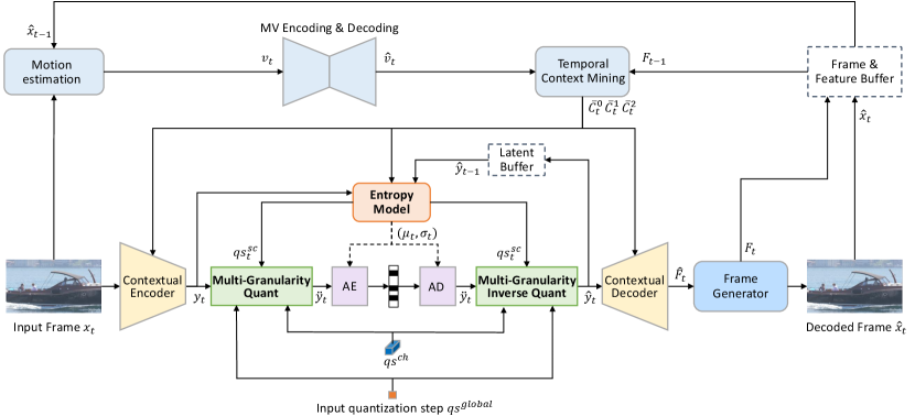
To achieve higher compression ratio for the input frame ( is the frame index), we adopt the conditional coding-based framework rather than the residual coding-based framework. Specifically, we follow the DCVC (Li et al., 2021) and its improved work (Sheng et al., 2021), and then redesign the core modules therein. The framework of our codec is presented in Fig. 1. As shown in this figure, the entire coding process can be roughly divided into three steps: temporal context generation, contextual encoding/decoding, and reconstruction.
Temporal context generation. To fully explore the temporal correlation, we generate the multi-scale contexts , , at different resolutions via the temporal context mining module (more details of this module can be found in (Sheng et al., 2021)). To carry richer information, we also use the temporal feature rather than previous decoded frame as the module input. As for motion estimation, we adopt the light-weight SPyNet (Ranjan and Black, 2017) for acceleration.
Contextual encoding/decoding. Conditioned by the multi-scale contexts, the current frame is transformed into latent representation by the contextual encoder. To achieve bitrate saving, the is quantized to before being sent to the arithmetic encoder which generates the bit-stream. During the decoding, is decoded from bit-steam by arithmetic decoder and inversely quantized to . Also conditioned on the multi-scale contexts, the contextual decoder decodes the high-resolution feature from . In this encoding/decoding process, how to accurately estimate the distribution of by the entropy model is vital for bitrate reduction. To this end, we propose the hybrid spatial-temporal entropy model (Section 3.2). To support smooth rate adjustment in single model, the multi-granularity quantization powered by our entropy model is proposed (Section 3.3).
Reconstruction. After obtaining the high-resolution feature , our target is generating the high-quality reconstructed frame via the frame generator. Different from DCVC (Li et al., 2021) and (Sheng et al., 2021) only using plain residual blocks (He et al., 2016), we proposing using the W-Net (Xia and Kulis, 2017) based structure which ties two U-Nets. Such kind of network design can effectively enlarge the receptive field of model with acceptable complexity. This results in stronger generation ability for model.
3.2. Hybrid Spatial-Temporal Entropy Model
For arithmetic coding, it needs to know the probability mass function (PMF) of to code it. However, we do not know its true PMF and usually approximate it with an estimated PMF . The cross-entropy captures the average number of bits needed by the arithmetic coding without considering the negligible overhead. In this paper, we follow the existing work (PyT, 2022) and assume that follows the Laplace distribution. Thus, our target is designing an entropy model which can accurately estimate the distribution parameter of to reduce the cross-entropy.
To improve the estimation, for each element (, , and are the height, width, and channel indexes) therein, we need to fully mine the correlation between it and its known information, e.g., the previous decoded latent representation, temporal context feature, and so on. Theoretically, may correlate to all these information from all previous decoded positions. For traditional codec, it is unable to explicitly exploit such correlation due to the huge space. Thus, traditional codec usually uses simple handcrafted rules to use context from a few neighbour positions. By contrast, the deep learning enables the capability of automatically mining the correlation in huge space.
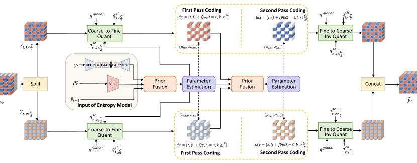
Thus, we propose feeding manifold inputs to the entropy model, and let the model extract the complementary information from the rich high-dimensional inputs. The illustration of our entropy model is shown in Fig. 2. As shown in this figure, the inputs not only contain the commonly-used hyper prior and the temporal context , but also include the as the latent prior. Although both and are from temporal direction, they have different characteristics. For example, at 4x down-sampled resolution usually contains lots of motion information (more details can be found in (Sheng et al., 2021)). By contrast, is in the latent representation domain at 16x down-sampled resolution, and has more similar characteristics with . Thus, and can provide the complementary auxiliary information to improve estimation. In addition, it is noted that we adopt the cascaded training strategy (Chan et al., 2021; Sheng et al., 2021), where the gradients will back propagate to multiple frames. Under such training strategy, the propagation chain of latent representation is formed. It means that the connection between the latent representation of the current frame and that of long-range reference frame is also built. Such connection is very helpful for extracting the correlation across the latent representation of multiple frames, and then results in more accurate prediction on distribution.
Besides using the latent prior to enrich the input, our entropy model also adopts the dual spatial prior to exploit the spatial correlation. To pursue a time-efficient mechanism, we follow the checkerboard model (He et al., 2021) rather than the commonly-used auto-regressive model (Minnen et al., 2018) which seriously slows down the coding speed. However, all channels in the original checkerboard model use the same coding order, namely the even positions are always first coded and then used as context for the coding of odd positions. Such coding order cannot handle various videos because sometimes coding the even positions first has worse RD performance than coding the odd positions first. Therefore, we design the dual spatial prior, where half channels in both even and odd positions are first coded at the same time.
As shown in Fig. 2, the latent representation is split into two chunks along the channel dimension. During the first-step coding, the above branch in Fig. 2 will code the even positions in the first chunk. Simultaneously, the below branch codes the odd positions in the second chunk. The uncoded positions (i.e., the white regions in Fig. 2) in these two chunks are set as zero. After the first-step coding, the coded and are fused together and then further generate the contexts for the second-step coding. During the second-step coding, the left positions in each chunk are coded. The above branch codes the odd positions in the first chunk and the below branch codes the even positions in the second chunk. As shown in Fig. 2, this coding manner enables that the second-step coding can benefit from the contexts from all positions. When compared with original checkerboard model (He et al., 2021), the scope of spatial context is doubled and results in more accurate prediction on distribution. It is noted that, for both steps, the first chunk and second chunk will be added and then sent to the arithmetic encoder. Thus, our dual spatial prior will not bring any additional coding delay when compared with (He et al., 2021).
In addition, from the perspective of channel dimension, our dual spatial prior also mines the correlation across channels. The coded during the first-step coding process can be also used as the condition for the coding of during the second-step coding process. It is similar for the coding of and , where the coding direction of channel is inverse. In a summary, our proposed dual spatial prior further squeezes the redundancy in by more efficiently exploiting the correlation across the spatial and channel positions.
3.3. Rate Adjustment in Single Model
It is a big pain that most existing neural codecs cannot handle rate adjustment in single model. To achieve different rates, the model needs to be retrained by adjusting the weight in the RD loss. It will bring large training cost and model storage burden. Such shortcoming calls for a mechanism supporting neural codec to achieve wide rate range in single model. To this end, we propose an adaptive quantization mechanism to enable this capability.
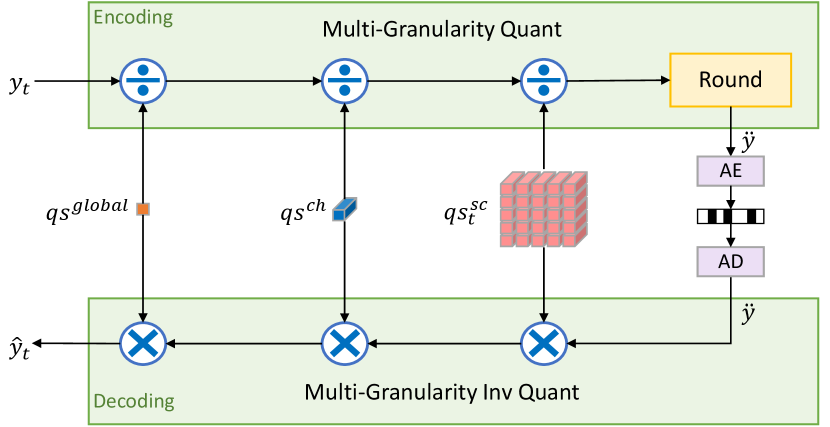
As shown in Fig. 3, our multi-granularity quantization involves three different kinds of quantization step (QP): the global QS , the channel-wise QS , and the spatial-channel-wise QS . The is only a single value and is set from the user input for controlling the target rate. As all positions take the same QS, the brings a coarse quantization effect. Thus, motivated by the channel attention mechanism (Hu et al., 2018), we also design a modulator to scale the QS at different channels because different channels carry information with different importance. However, the different spatial positions also have different characteristics due to the various video contents. Thus, we follow (Huang et al., 2022) and learn the spatial-channel-wise to achieve the precise adjustment on each position.
| UVG | MCL-JCV | HEVC B | HEVC C | HEVC D | HEVC E | HEVC RGB | Average | |
|---|---|---|---|---|---|---|---|---|
| VTM-13.2 | 0.0 | 0.0 | 0.0 | 0.0 | 0.0 | 0.0 | 0.0 | 0.0 |
| HM-16.20 | 40.5 | 45.4 | 40.4 | 40.9 | 36.0 | 46.2 | 42.1 | 41.6 |
| x265 | 191.5 | 160.3 | 143.4 | 105.2 | 96.1 | 128.4 | 151.2 | 139.4 |
| DVCPro (Lu et al., 2020b) | 227.0 | 180.8 | 209.8 | 220.6 | 166.4 | 446.2 | 178.5 | 232.8 |
| RLVC (Yang et al., 2021a) | 224.2 | 214.3 | 207.0 | 212.4 | 149.2 | 392.8 | 195.5 | 227.9 |
| MLVC (Lin et al., 2020) | 113.6 | 124.0 | 118.0 | 213.7 | 166.5 | 237.6 | 151.2 | 160.7 |
| DCVC (Li et al., 2021) | 126.1 | 98.2 | 115.0 | 150.8 | 109.6 | 266.2 | 109.6 | 139.4 |
| Sheng 2021 (Sheng et al., 2021) | 17.1 | 30.6 | 28.5 | 60.5 | 27.8 | 67.3 | 17.9 | 35.7 |
| Ours | –18.2 | –6.4 | –5.1 | 15.0 | –8.9 | 7.1 | –16.4 | –4.7 |
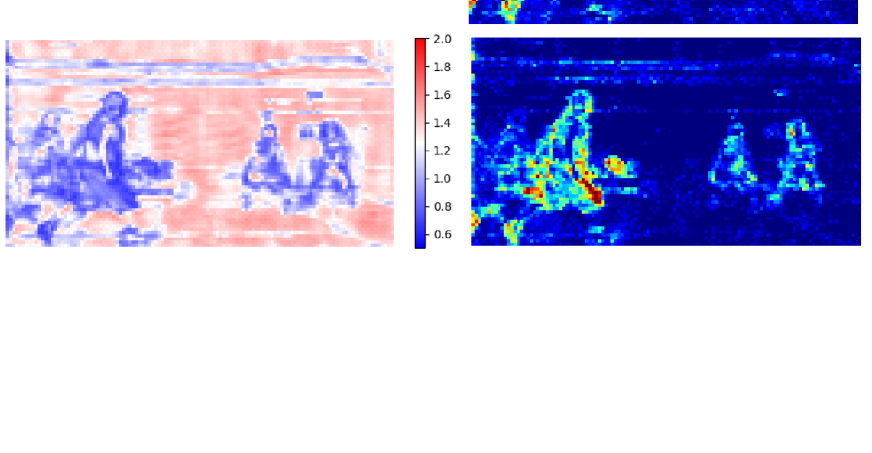
The is generated by our entropy model, as shown in Fig. 2. It is noted that, for each frame, it is dynamically changed to adapt the video contents. Such design not only helps us achieve smooth rate adjustment but also improves the final RD performance by content-adaptive bit allocation. The important information which is vital for the reconstruction or is referenced by the coding of the subsequent frames will be allocated with smaller QS. We show a visualization example of in Fig. 4. In this example, the model learns that the moving players are more important and produces smaller QS for these regions. By contrast, the backgrounds have larger QS, which brings considerable bitrate saving (as shown in region indicated by the yellow line). The ablation study in section 4.3 shows can achieve substantial improvements on multiple datasets.
During the decoding, the corresponding inverse quantization is applied. It is noted that, the needs to be transmitted to the decoder along with the bit-stream. However, this overhead is negligible as only single number is transmitted for each frame or video (flexible setting for user). The modulator belongs to a part of our neural codec and is learned during the training.
4. Experimental Results
4.1. Experimental Setup
Datasets. We use Vimeo-90k (Xue et al., 2019) for training. The videos are randomly cropped into 256x256 patches. For testing, we use the same test videos as (Sheng et al., 2021). All these test videos are widely used in the evaluation of traditional and neural video codecs, including HEVC Class B, C, D, E, and RGB. In addition, the 1080p videos from UVG (Mercat et al., 2020) and MCL-JCV (Wang et al., 2016) datasets are also tested.
Test conditions. We test 96 frames for each video. The intra period is set to 32 rather than 10 or 12. The reason is that intra period 32 gets closer to the practical usage in the real applications. For example, when compared with intra period 12, intra period 32 has an average of 23.8% (Sheng et al., 2021) bitrate saving for HM. We follow the low delay encoding settings as most existing works (Lu et al., 2019, 2020b; Li et al., 2021; Sheng et al., 2021). The compression ratio is measured by BD-Rate (Bjontegaard, 2001), where negative numbers indicate bitrate saving and positive numbers indicate bitrate increase.
Besides x265 (x26, 2022) (veryslow preset is used), our benchmarks include HM-16.20 (HM, 2022) and VTM-13.2 (VTM, 2022), which represent the best encoder of H.265 and H.266, respectively. For HM and VTM, we follow (Sheng et al., 2021) and use the configuration with the highest compression ratio. We also compare previous SOTA neural video codecs including DVCPro (Lu et al., 2020b), MLVC (Lin et al., 2020), RLVC (Yang et al., 2021a), DCVC (Li et al., 2021), as well as Sheng 2021 (Sheng et al., 2021).
| UVG | MCL-JCV | HEVC B | HEVC C | HEVC D | HEVC E | HEVC RGB | Average | |
|---|---|---|---|---|---|---|---|---|
| VTM-13.2 | 0.0 | 0.0 | 0.0 | 0.0 | 0.0 | 0.0 | 0.0 | 0.0 |
| HM-16.20 | 36.9 | 43.7 | 36.7 | 38.7 | 34.9 | 40.5 | 37.2 | 38.4 |
| x265 | 150.5 | 137.6 | 129.3 | 109.5 | 101.8 | 109.0 | 121.9 | 122.8 |
| DVCPro (Lu et al., 2020b) | 68.1 | 37.8 | 61.7 | 59.1 | 23.9 | 212.5 | 57.3 | 74.3 |
| RLVC (Yang et al., 2021a) | 83.9 | 72.1 | 66.6 | 76.5 | 34.1 | 268.4 | 60.5 | 94.6 |
| DCVC (Li et al., 2021) | 33.6 | 4.7 | 31.0 | 22.8 | 1.2 | 124.7 | 36.5 | 36.4 |
| Sheng 2021 (Sheng et al., 2021) | –10.1 | –24.4 | –24.1 | –23.3 | –37.3 | –8.0 | –25.9 | –21.9 |
| Ours | –35.1 | –46.8 | –48.1 | –44.6 | –55.7 | –47.5 | –47.0 | –46.4 |
Implementation and training details. The entropy model and quantization for the latent representation of motion vector follow those of . The only difference is the input of entropy model. In the coding of motion vector, the inputs are the corresponding hyper prior and the latent prior, i.e., the quantized latent representation of motion vector from the previous frame. There is no temporal context prior for the coding of motion vector because the generation of temporal context depends on the decoded motion vector. In addition, as we target at single model handling multiple rates, we also train a neural image codec supporting such capability for intra coding.
During the training, the loss function includes the distortion and rate: . refers to the distortion between the input frame and the reconstructed frame. The distortion can be loss or MS-SSIM (Wang et al., 2003) for different visual targets. represents the bits used for encoding and the quantized latent representation of motion vector, both associated with the bits used for encoding their corresponding hyper prior.
We adopt the multi-stage training, same as (Sheng et al., 2021). In addition, to train single model supporting rate adjustment, we use different values in different optimization steps. For simplifying the training process, 4 values (85, 170, 380, 840) are used. During the training, 4 values will be learned via the RD loss with each corresponding value. We trained image and video models separately and they have different values. It is noted that, although we only use 4 values during the training, the model still can achieve smooth rate adjustment by manually adjusting the during the testing, and the corresponding study is presented in Section 4.4.
4.2. Comparisons with Previous SOTA Methods
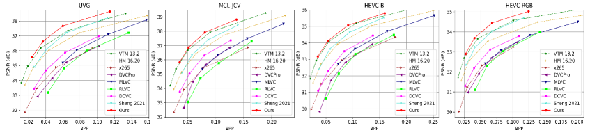
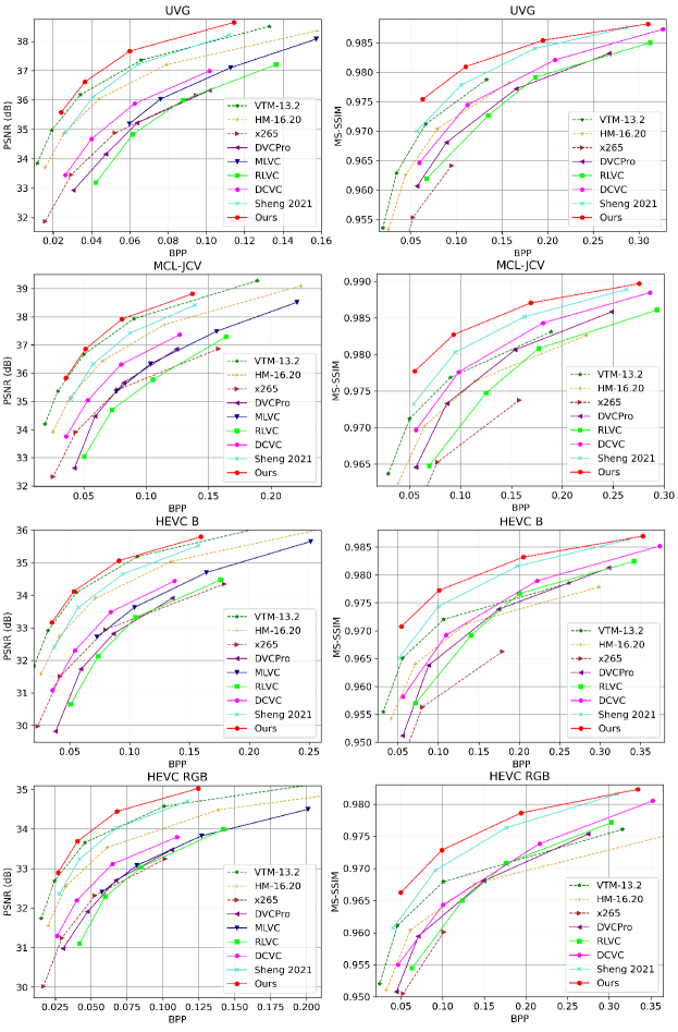
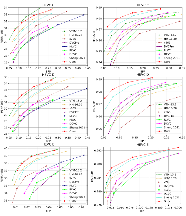
Table 1 and Table 2 show the BD-Rate (%) comparisons in terms of PSNR and MS-SSIM, respectively. The best traditional codec VTM is used as anchor. From Table 1, we can find that our neural codec achieves an average of 4.7% bitrate saving over VTM on all datasets. By contrast, the second best method Sheng 2021 (Sheng et al., 2021) is far behind than VTM and has 35.7% bitrate increase. To the best of our knowledge, this is the first end-to-end neural video codec that outperforms VTM using the highest compression ratio configuration, which is an important milestone in the development of neural video codec. In particular, our neural codec performs better for 1080p videos (HEVC B, HEVC RGB, UVG, MCL-JCV). Fig. 5 shows RD curves on these datasets. We can find our codec consumes the least bits under the same quality. These results verify the effectiveness of our entropy model on exploiting the correlation among the volumed video data. In addition, the high-resolution video will be more popular in the future and the advantage of our neural codec will be more obvious. When oriented to MS-SSIM, our neural video codec has larger improvement. As shown in Table 2, we achieve an average of 46.4% bitrate saving over VTM on all datasets.
4.3. Ablation Study
To verify the effectiveness of each component, we conduct a comprehensive ablation study. We analyze the effect of entropy model input, our dual spatial prior, the multi-granularity quantization, as well as the design on frame generator. For simplification, we only use HEVC testsets in ablation study. The comparisons are measured by BD-Rate (%).
| Hyper | Temporal | Latent | B | C | D | E | RGB | Average |
| prior | context prior | prior | ||||||
| ✓ | ✓ | ✓ | 0.0 | 0.0 | 0.0 | 0.0 | 0.0 | 0.0 |
| ✓ | ✓ | ✗ | 9.5 | 5.6 | 6.4 | 18.4 | 10.7 | 10.1 |
| ✓ | ✗ | ✓ | 9.2 | 8.8 | 9.1 | 15.0 | 9.1 | 10.2 |
| ✗ | ✓ | ✓ | 19.5 | 9.1 | 11.9 | 27.2 | 20.9 | 17.7 |
| ✓ | ✗ | ✗ | 12.4 | 14.7 | 17.9 | 23.4 | 9.4 | 15.6 |
| ✗ | ✓ | ✗ | 33.8 | 29.3 | 31.6 | 54.3 | 36.2 | 37.0 |
| ✗ | ✗ | ✓ | 19.5 | 19.3 | 19.2 | 21.1 | 17.3 | 19.3 |
The inputs of entropy model. As shown in Fig. 2, our entropy model contains three different kinds of inputs: hyper prior, temporal context prior, and latent prior. Table 3 compares the effectiveness of these inputs. When removing our latent prior, there is 10.1% bitrate increase. If only enabling one prior input, the first and second most important inputs are hyper prior (15.6%) and our latent prior (19.3%). From these comparisons, we can find that the hyper prior is still the most important. But enriching the entropy model input via our latent prior also brings significant bitrate saving.
Different spatial priors. Table 4 compares the effect of different spatial prior modules on exploring the inner correlation in . The tested spatial context models include our proposed dual spatial prior, checkerboard prior (He et al., 2021), and the parallel-unfriendly auto-regressive prior (Minnen et al., 2018). From this table, we can find that our dual spatial prior could bring 14.1% bitrate saving. And there is 6.2% improvement over the checkerboard prior. This verifies the benefit of enlarging the scope of spatial context and exploiting the cross-channel correlation. In addition, we also find that the auto-regressive prior could further save the bitrate by a large margin (12.0%). However, considering the very slow encoding and decoding speed, we still do not adopt it in our neural codec.
| B | C | D | E | RGB | Average | |
|---|---|---|---|---|---|---|
| Proposed dual spatial prior | 0.0 | 0.0 | 0.0 | 0.0 | 0.0 | 0.0 |
| Checkerboard prior | 5.6 | 4.1 | 6.0 | 11.0 | 5.5 | 6.2 |
| No spatial prior | 11.9 | 11.1 | 11.6 | 29.7 | 6.4 | 14.1 |
| Auto-regressive prior | –14.8 | –11.4 | –11.2 | –5.6 | –16.9 | –12.0 |
Multi-granularity quantization. As introduced in Section 3.3, the multi-granularity quantization powered by our entropy model not only helps us achieve rate adjustment in single model but also improves the final RD performance by content-adaptive bit allocation. Table 5 shows the BD-rate comparison. From this table, we can find that there is 11.8% loss if disabling the whole multi-granularity quantization. When only removing the spatial-channel-wise quantization step , there is a significant 8.9% bit increase. It shows that the play an important role in multi-granularity quantization and it is necessary to design a dynamic bit allocation which can adapt to various video contents.
| B | C | D | E | RGB | Average | |
|---|---|---|---|---|---|---|
| Multi-granularity quantization | 0.0 | 0.0 | 0.0 | 0.0 | 0.0 | 0.0 |
| w/o | 9.7 | 10.1 | 10.6 | 8.3 | 5.6 | 8.9 |
| w/o multi-granularity quantization | 9.9 | 15.1 | 14.6 | 11.7 | 7.8 | 11.8 |
Frame generator design. To improve the generation ability of neural codec, our frame generator uses W-Net based structure to enlarge the receptive field. To verify its effectiveness, we compare the frame generator using different networks, as shown in Table 6. We compare W-Net, U-Net, and residual block (Li et al., 2021; Sheng et al., 2021) based structures. From this table, we can find that W-Net has more than 10% bitrate saving than the plain network using residual blocks. The W-Net which ties two U-Nets is also 7.9% better than the single U-Net. Thus, it is possible that larger bitrate saving can be achieved by using more U-Nets. However, considering the complexity, we currently use W-Net.
4.4. Smooth Rate Adjustment in Single Model
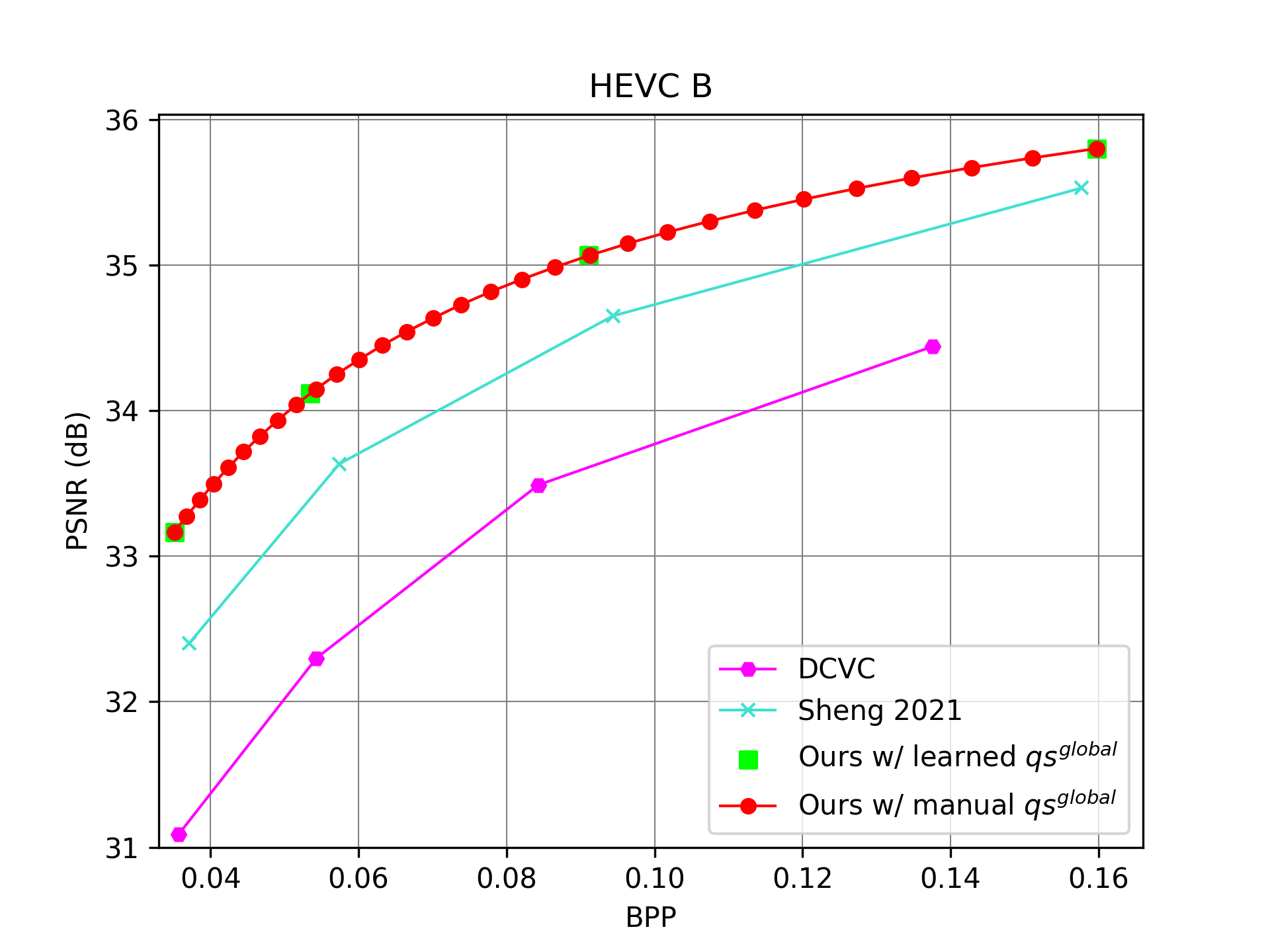
Table 5 shows the RD improvement of multi-granularity quantization. This sub-section investigates whether our multi-granularity quantization can achieve smooth rate adjustment. For our codec, the global quantization step can be flexibly adjusted during the testing. It serves the similar role of quantization parameter in traditional video codecs. Fig. 6 shows the results of our codec using the learned 4 values which are guided by RD loss using the 4 values during the training. In addition, we also manually generate 30 values by the interpolation between the maximum and minimum of the learned values. From the results at the 30 rate points, we can find that our single model could achieve smooth rate adjustment without any outlier. By contrast, DCVC (Li et al., 2021) and Sheng 2021 (Sheng et al., 2021) need different models for each rate point.
4.5. Model Complexity
We compare the model complexity in model size, MACs (multiply–accumulate operations), encoding time, and decoding time with previous SOTA neural video codecs, as shown in Table 7. We use 1080p frame as input to measure these numbers. For the encoding/decoding time, we measure the time on NVIDIA V100 GPU, including the time of writing to and reading from bitstream as in (Sheng et al., 2021). As aforementioned, our model supports rate adjustment in single model. Thus, we significantly reduce the model training and storage burden. Because DCVC (Li et al., 2021) uses the parallel-unfriendly auto-regression prior model, its encoding/decoding time is quite slow. By contrast, (Sheng et al., 2021) and our codec are much faster. Compare with (Sheng et al., 2021), our encoding/decoding time is increased a little. However, the compression ratio is pushed into a new height (from Sheng 2021 surpassing HM to ours surpassing VTM). We believe this is a price worth paying.
5. Conclusion
In this paper, we have presented how to design an efficient entropy model which helps our neural codec not only achieve the higher compression ratio than VTM but also smoothly adjust the rates in single model. In particular, the latent prior is proposed to enrich the input of entropy model. Via building the the propagation chain, the model can exploit the correlation across the latent representation of multiple frames. The proposed dual spatial prior not only doubles the scope of spatial context in parallel-friendly manner but also further squeezes the redundancy across the channel dimension. In addition, our entropy model also generates the spatial-channel-wise quantization step. Such content-adaptive quantization mechanism helps the codec cope with various video consents well. As the core element in the multi-granularity quantization, it not only helps achieve the smooth rate adjustment but also improves the final RD performance by dynamic bit allocation. When compared with the best traditional codec VTM using the highest compression ratio configuration, an average of 18.2% bitrate saving is achieved on UVG dataset, which is an important milestone.
References
- (1)
- HM (2022) 2022. HM-16.20. https://vcgit.hhi.fraunhofer.de/jvet/HM/. Accessed: 2022-03-02.
- PyT (2022) 2022. PyTorchVideoCompression. https://github.com/ZhihaoHu/PyTorchVideoCompression. Accessed: 2022-03-02.
- uvg (2022) 2022. Ultra video group test sequences. http://ultravideo.cs.tut.fi. Accessed: 2022-03-02.
- VTM (2022) 2022. VTM-13.2. https://vcgit.hhi.fraunhofer.de/jvet/VVCSoftware_VTM/. Accessed: 2022-03-02.
- x26 (2022) 2022. x265. https://www.videolan.org/developers/x265.html. Accessed: 2022-03-02.
- Agustsson et al. (2020) Eirikur Agustsson, David Minnen, Nick Johnston, Johannes Balle, Sung Jin Hwang, and George Toderici. 2020. Scale-space flow for end-to-end optimized video compression. In Proceedings of the IEEE/CVF Conference on Computer Vision and Pattern Recognition. 8503–8512.
- Ballé et al. (2017) Johannes Ballé, Valero Laparra, and Eero P. Simoncelli. 2017. End-to-end Optimized Image Compression. In 5th International Conference on Learning Representations, ICLR 2017.
- Ballé et al. (2018) Johannes Ballé, David Minnen, Saurabh Singh, Sung Jin Hwang, and Nick Johnston. 2018. Variational image compression with a scale hyperprior. 6th International Conference on Learning Representations, ICLR (2018).
- Bjontegaard (2001) Gisle Bjontegaard. 2001. Calculation of average PSNR differences between RD-curves. VCEG-M33 (2001).
- Bross et al. (2021) Benjamin Bross, Ye-Kui Wang, Yan Ye, Shan Liu, Jianle Chen, Gary J Sullivan, and Jens-Rainer Ohm. 2021. Overview of the versatile video coding (VVC) standard and its applications. IEEE Transactions on Circuits and Systems for Video Technology 31, 10 (2021), 3736–3764.
- Chan et al. (2021) Kelvin CK Chan, Xintao Wang, Ke Yu, Chao Dong, and Chen Change Loy. 2021. BasicVSR: The search for essential components in video super-resolution and beyond. In Proceedings of the IEEE/CVF Conference on Computer Vision and Pattern Recognition. 4947–4956.
- Cheng et al. (2020) Zhengxue Cheng, Heming Sun, Masaru Takeuchi, and Jiro Katto. 2020. Learned image compression with discretized gaussian mixture likelihoods and attention modules. In Proceedings of the IEEE/CVF Conference on Computer Vision and Pattern Recognition. 7939–7948.
- Cui et al. (2021) Ze Cui, Jing Wang, Shangyin Gao, Tiansheng Guo, Yihui Feng, and Bo Bai. 2021. Asymmetric gained deep image compression with continuous rate adaptation. In Proceedings of the IEEE/CVF Conference on Computer Vision and Pattern Recognition. 10532–10541.
- Djelouah et al. (2019) Abdelaziz Djelouah, Joaquim Campos, Simone Schaub-Meyer, and Christopher Schroers. 2019. Neural Inter-Frame Compression for Video Coding. In Proceedings of the IEEE/CVF International Conference on Computer Vision (ICCV).
- Habibian et al. (2019) Amirhossein Habibian, Ties van Rozendaal, Jakub M Tomczak, and Taco S Cohen. 2019. Video compression with rate-distortion autoencoders. In Proceedings of the IEEE/CVF International Conference on Computer Vision. 7033–7042.
- He et al. (2021) Dailan He, Yaoyan Zheng, Baocheng Sun, Yan Wang, and Hongwei Qin. 2021. Checkerboard context model for efficient learned image compression. In Proceedings of the IEEE/CVF Conference on Computer Vision and Pattern Recognition. 14771–14780.
- He et al. (2016) Kaiming He, Xiangyu Zhang, Shaoqing Ren, and Jian Sun. 2016. Deep residual learning for image recognition. In Proceedings of the IEEE conference on computer vision and pattern recognition. 770–778.
- Hu et al. (2018) Jie Hu, Li Shen, and Gang Sun. 2018. Squeeze-and-excitation networks. In Proceedings of the IEEE conference on computer vision and pattern recognition. 7132–7141.
- Hu et al. (2020) Zhihao Hu, Zhenghao Chen, Dong Xu, Guo Lu, Wanli Ouyang, and Shuhang Gu. 2020. Improving deep video compression by resolution-adaptive flow coding. In European Conference on Computer Vision. Springer, 193–209.
- Hu et al. (2021) Zhihao Hu, Guo Lu, and Dong Xu. 2021. FVC: A New Framework towards Deep Video Compression in Feature Space. In Proceedings of the IEEE/CVF Conference on Computer Vision and Pattern Recognition (CVPR). 1502–1511.
- Huang et al. (2022) Cong Huang, Jiahao Li, Bin Li, Dong Liu, and Yan Lu. 2022. Neural Compression-Based Feature Learning for Video Restoration. In Proceedings of the IEEE/CVF Conference on Computer Vision and Pattern Recognition (CVPR). 5872–5881.
- Hui et al. (2020) Tak-Wai Hui, Xiaoou Tang, and Chen Change Loy. 2020. A lightweight optical flow CNN—Revisiting data fidelity and regularization. IEEE transactions on pattern analysis and machine intelligence 43, 8 (2020), 2555–2569.
- Koyuncu et al. (2022) A Burakhan Koyuncu, Han Gao, and Eckehard Steinbach. 2022. Contextformer: A Transformer with Spatio-Channel Attention for Context Modeling in Learned Image Compression. arXiv preprint arXiv:2203.02452 (2022).
- Ladune et al. (2020) Théo Ladune, Pierrick Philippe, Wassim Hamidouche, Lu Zhang, and Olivier Déforges. 2020. Optical Flow and Mode Selection for Learning-based Video Coding. In 22nd IEEE International Workshop on Multimedia Signal Processing.
- Ladune et al. (2021a) Théo Ladune, Pierrick Philippe, Wassim Hamidouche, Lu Zhang, and Olivier Déforges. 2021a. Conditional Coding and Variable Bitrate for Practical Learned Video Coding. CLIC workshop, CVPR (2021).
- Ladune et al. (2021b) Théo Ladune, Pierrick Philippe, Wassim Hamidouche, Lu Zhang, and Olivier Déforges. 2021b. Conditional Coding for Flexible Learned Video Compression. In Neural Compression: From Information Theory to Applications – Workshop @ ICLR.
- Li et al. (2021) Jiahao Li, Bin Li, and Yan Lu. 2021. Deep contextual video compression. Advances in Neural Information Processing Systems 34 (2021).
- Lin et al. (2020) Jianping Lin, Dong Liu, Houqiang Li, and Feng Wu. 2020. M-LVC: multiple frames prediction for learned video compression. In Proceedings of the IEEE/CVF Conference on Computer Vision and Pattern Recognition.
- Liu et al. (2020a) Haojie Liu, Ming Lu, Zhan Ma, Fan Wang, Zhihuang Xie, Xun Cao, and Yao Wang. 2020a. Neural video coding using multiscale motion compensation and spatiotemporal context model. IEEE Transactions on Circuits and Systems for Video Technology (2020).
- Liu et al. (2020b) Haojie Liu, Han Shen, Lichao Huang, Ming Lu, Tong Chen, and Zhan Ma. 2020b. Learned video compression via joint spatial-temporal correlation exploration. In Proceedings of the AAAI Conference on Artificial Intelligence, Vol. 34. 11580–11587.
- Liu et al. (2020c) Jerry Liu, Shenlong Wang, Wei-Chiu Ma, Meet Shah, Rui Hu, Pranaab Dhawan, and Raquel Urtasun. 2020c. Conditional entropy coding for efficient video compression. In European Conference on Computer Vision. Springer, 453–468.
- Lu et al. (2020a) Guo Lu, Chunlei Cai, Xiaoyun Zhang, Li Chen, Wanli Ouyang, Dong Xu, and Zhiyong Gao. 2020a. Content adaptive and error propagation aware deep video compression. In European Conference on Computer Vision. Springer, 456–472.
- Lu et al. (2019) Guo Lu, Wanli Ouyang, Dong Xu, Xiaoyun Zhang, Chunlei Cai, and Zhiyong Gao. 2019. DVC: an end-to-end deep video compression framework. In Proceedings of the IEEE/CVF Conference on Computer Vision and Pattern Recognition. 11006–11015.
- Lu et al. (2020b) Guo Lu, Xiaoyun Zhang, Wanli Ouyang, Li Chen, Zhiyong Gao, and Dong Xu. 2020b. An end-to-end learning framework for video compression. IEEE transactions on pattern analysis and machine intelligence (2020).
- Mercat et al. (2020) Alexandre Mercat, Marko Viitanen, and Jarno Vanne. 2020. UVG dataset: 50/120fps 4K sequences for video codec analysis and development. In Proceedings of the 11th ACM Multimedia Systems Conference. 297–302.
- Minnen et al. (2018) David Minnen, Johannes Ballé, and George D Toderici. 2018. Joint autoregressive and hierarchical priors for learned image compression. Advances in neural information processing systems 31 (2018).
- Pessoa et al. (2020) Jorge Pessoa, Helena Aidos, Pedro Tomás, and Mário AT Figueiredo. 2020. End-to-end learning of video compression using spatio-temporal autoencoders. In 2020 IEEE Workshop on Signal Processing Systems (SiPS). IEEE, 1–6.
- Ranjan and Black (2017) Anurag Ranjan and Michael J Black. 2017. Optical flow estimation using a spatial pyramid network. In Proceedings of the IEEE conference on computer vision and pattern recognition. 4161–4170.
- Rippel et al. (2021) Oren Rippel, Alexander G Anderson, Kedar Tatwawadi, Sanjay Nair, Craig Lytle, and Lubomir Bourdev. 2021. ELF-VC: Efficient Learned Flexible-Rate Video Coding. In Proceedings of the IEEE/CVF International Conference on Computer Vision (ICCV). 14479–14488.
- Rippel et al. (2019) Oren Rippel, Sanjay Nair, Carissa Lew, Steve Branson, Alexander G Anderson, and Lubomir Bourdev. 2019. Learned video compression. In Proceedings of the IEEE/CVF International Conference on Computer Vision. 3454–3463.
- Sheng et al. (2021) Xihua Sheng, Jiahao Li, Bin Li, Li Li, Dong Liu, and Yan Lu. 2021. Temporal Context Mining for Learned Video Compression. arXiv preprint arXiv:2111.13850 (2021).
- Sun et al. (2020) Wenyu Sun, Chen Tang, Weigui Li, Zhuqing Yuan, Huazhong Yang, and Yongpan Liu. 2020. High-Quality Single-Model Deep Video Compression with Frame-Conv3D and Multi-frame Differential Modulation. In European Conference on Computer Vision (ECCV). Springer, 239–254.
- Theis et al. (2017) Lucas Theis, Wenzhe Shi, Andrew Cunningham, and Ferenc Huszár. 2017. Lossy image compression with compressive autoencoders. 5th International Conference on Learning Representations, ICLR (2017).
- Wang et al. (2016) Haiqiang Wang, Weihao Gan, Sudeng Hu, Joe Yuchieh Lin, Lina Jin, Longguang Song, Ping Wang, Ioannis Katsavounidis, Anne Aaron, and C-C Jay Kuo. 2016. MCL-JCV: a JND-based H. 264/AVC video quality assessment dataset. In 2016 IEEE International Conference on Image Processing (ICIP). IEEE, 1509–1513.
- Wang et al. (2003) Zhou Wang, Eero P Simoncelli, and Alan C Bovik. 2003. Multiscale structural similarity for image quality assessment. In The Thrity-Seventh Asilomar Conference on Signals, Systems & Computers, 2003, Vol. 2. Ieee, 1398–1402.
- Wu et al. (2018) Chao-Yuan Wu, Nayan Singhal, and Philipp Krahenbuhl. 2018. Video compression through image interpolation. In Proceedings of the European Conference on Computer Vision (ECCV). 416–431.
- Xia and Kulis (2017) Xide Xia and Brian Kulis. 2017. W-net: A deep model for fully unsupervised image segmentation. arXiv preprint arXiv:1711.08506 (2017).
- Xue et al. (2019) Tianfan Xue, Baian Chen, Jiajun Wu, Donglai Wei, and William T Freeman. 2019. Video Enhancement with Task-Oriented Flow. International Journal of Computer Vision (IJCV) 127, 8 (2019), 1106–1125.
- Yang et al. (2021a) Ren Yang, Fabian Mentzer, Luc Van Gool, and Radu Timofte. 2021a. Learning for Video Compression with Recurrent Auto-Encoder and Recurrent Probability Model. IEEE Journal of Selected Topics in Signal Processing 15, 2 (2021), 388–401.
- Yang et al. (2021b) Ruihan Yang, Yibo Yang, Joseph Marino, and Stephan Mandt. 2021b. Hierarchical autoregressive modeling for neural video compression. 9th International Conference on Learning Representations, ICLR (2021).
Appendices provide the supplementary material to our proposed hybrid spatial-temporal entropy modelling for neural video compression.
Appendix A Network Architecture
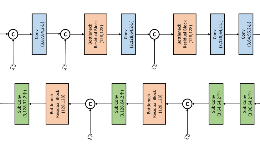
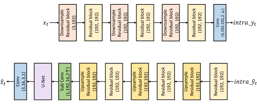
Contextual encoder and decoder. The network design of our contextual encoder and decoder is shown in Fig. 7. For encoder, the inputs are the current original frame and the multi-scale contexts , , at different resolutions (original, 2x downsampled, 4x downsampled) with channel 64. The output is the latent representation with channel 96 at 16x downsampled resolution. For decoder, the inputs contain the decoded latent representation . Conditioned on and , the high-resolution feature with channel 32 is decoded. For the convolutional and sub-pixel convolutional layers in Fig. 7, the indicate the kernel size, input channel number, output channel number, and stride, respectively. In Fig. 7, the bottleneck residual block comes from (Sheng et al., 2021). The kernel size and stride of convolutional layer therein are 3 and 1, respectively. Thus, we only show the input and output channel numbers for bottleneck residual block.
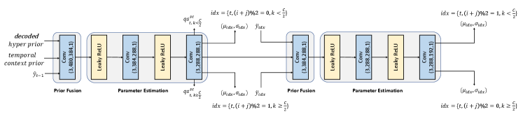
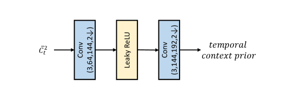
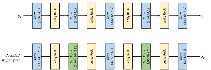
Entropy model. Fig. 8 shows the detailed network structure of our entropy model. The inputs include the the hyper prior with channel 192, the temporal context prior with channel 192, the latent prior (i.e., the decoded latent representation from the previous frame) with channel 96. The temporal context prior is generated by the temporal context encoder, as shown in Fig. 9. The network structures of hyper prior encoder and decoder are shown in Fig. 10.
In the first-step coding, the entropy model not only estimates the mean and scale values of the probability distribution for the quantized latent representations and , but also generates the quantization step at spatial-channel-wise. During the second-step coding, the coded latent representations in previous step are fused to the input, and then the entropy model estimates the the mean and scale values of the probability distribution for and .
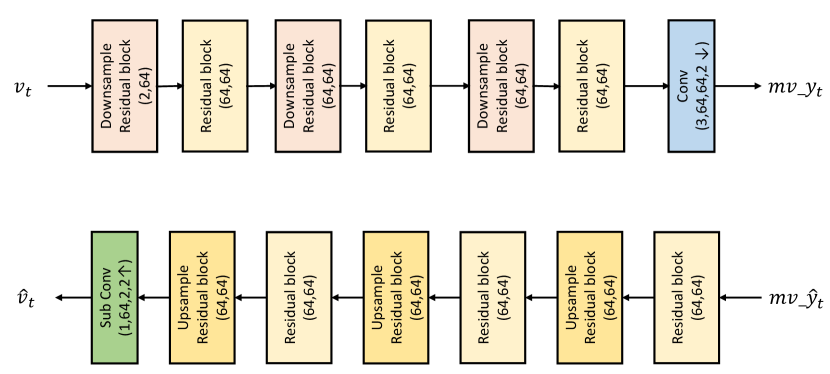
Motion vector encoder and decoder. The encoder and decoder for motion vector are illustrated in Fig. 11. For encoder, the input is the original motion vector with channel 2. The output is the latent representation at 16x downsampled resolution with channel 64. The decoder follows the inverse structure. The multi-granularity quantization and entropy model for follow those of . The only difference is the entropy model input. For motion vector, the inputs of entropy model are the corresponding hyper prior and the latent prior. In Fig. 11, the downsample and upsample residual blocks are from (Sheng et al., 2021).
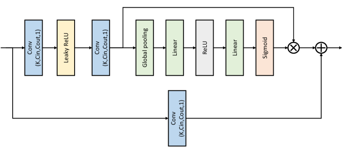
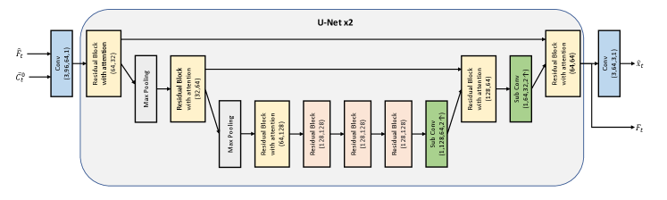
Frame generator. Different from DCVC (Li et al., 2021) and (Sheng et al., 2021) only using plain residual blocks, we proposing using the W-Net (Xia and Kulis, 2017) based structure to build our frame generator. The W-Net can effectively enlarge the receptive field of model to improve the generation ability of model. The detailed network structure of our frame generator is presented in Fig. 14. The inputs include the the high-resolution feature with channel 32 and the context at original resolution with channel 64. The outputs are the final reconstructed frame and the feature used by the next frame. In Fig. 14, there are two same U-Nets to build the W-Net. The residual block with attention in the U-Net is illustrated in Fig.12.
Neural image codec. As we target at single model handling multiple rates, we also need a neural image codec supporting such capability for intra coding. The structure of our neural image codec is presented in Fig. 13. The corresponding multi-granularity quantization and the entropy model are similar with those of . The only difference is the input of entropy model. For neural image codec, the input of entropy model only includes the hyper prior. In Fig. 13, we also use one U-Net to improve the generation ability of neural image codec and its network structure is similar to that in Fig. 14. The compression ratio of our image codec is on par with that of Cheng 2020 (Cheng et al., 2020), as shown in Table 8.
Appendix B Settings of Traditional Codecs
For x265 (x26, 2022), we use the veryslow preset. We also compare HM-16.20 (HM, 2022) and VTM-13.2 (VTM, 2022), which represent the best encoder of H.265 and H.266, respectively. For HM and VTM, the low delay configuration with the highest compression ratio is used. 4 reference frames and 10-bit internal bit depth are used (settings in encoder_lowdelay_main_rext.cfg for HM and encoder_lowdelay_vtm.cfg for VTM). The comparison in (Sheng et al., 2021) has shown that, although the final distortion is measured in RGB domain, using YUV 444 as the internal color space could boost the compression ratio. Thus, we also use this setting. More studies on codec setting can be found in (Sheng et al., 2021). The detailed settings of x265, HM, and VTM are:
-
•
x265
ffmpeg
-pix_fmt yuv420p
-s {width}x{height}
-framerate {frame rate}
-i {input file name}
-vframes {frame number}
-c:v libx265
-preset veryslow
-tune zerolatency
-x265-params
“qp={qp}:keyint=32:csv-log-level=1:
csv={csv_path}:verbose=1:psnr=1”
{output video file name}
-
•
HM
TAppEncoder
-c encoder_lowdelay_main_rext.cfg
–InputFile={input file name}
–InputBitDepth=8
–OutputBitDepth=8
–OutputBitDepthC=8
–InputChromaFormat=444
–FrameRate={frame rate}
–DecodingRefreshType=2
–FramesToBeEncoded={frame number}
–SourceWidth={width}
–SourceHeight={height}
–IntraPeriod=32
–QP={qp}
–Level=6.2
–BitstreamFile={bitstream file name}
-
•
VTM
EncoderApp
-c encoder_lowdelay_vtm.cfg
–InputFile={input file name}
–BitstreamFile={bitstream file name}
–DecodingRefreshType=2
–InputBitDepth=8
–OutputBitDepth=8
–OutputBitDepthC=8
–InputChromaFormat=444
–FrameRate={frame rate}
–FramesToBeEncoded={frame number}
–SourceWidth={width}
–SourceHeight={height}
–IntraPeriod=32
–QP={qp}
–Level=6.2
| UVG | MCL-JCV | HEVC B | HEVC C | HEVC D | HEVC E | HEVC RGB | Average | |
|---|---|---|---|---|---|---|---|---|
| Cheng 2020 image codec (Cheng et al., 2020) | 0.0 | 0.0 | 0.0 | 0.0 | 0.0 | 0.0 | 0.0 | 0.0 |
| Our image codec | -0.9 | 0.2 | -1.9 | -0.2 | 2.5 | 1.9 | -1.2 | 0.1 |
Appendix C Rate-Distortion Curves
Fig. 15 and Fig. 16 show the RD (rate-distortion) curves on each dataset, including both the PSNR and MS-SSIM results. From these results, we can find that our codec can achieve SOTA compression ratio in wide rate range.
Appendix D Comparison under Different Intra Period Settings
Previous work Sheng 2021 (Sheng et al., 2021) shows that intra period 12 is harmful to the compression ratio and is seldom used in the real applications. For example, when compared with intra period 12, intra period 32 has an average of 23.8% bitrate saving for HM (Table 3 in the supplementary material of (Sheng et al., 2021)). Thus, to get closer to the practical scenario, we follow [39] and also use intra period 32 in our paper.
But it is also important to evaluate our codec under intra period 12. Table 9 shows the corresponding BD-rate (%) comparison in terms of PSNR. It is noted that, since the GOP size of VTM with *encoder_lowdelay_vtm* configuration is 8, it does not support intra period 12. Therefore, we configure VTM-13.2* by following (Sheng et al., 2021) and use it as the anchor (more configuration details of VTM-13.2* can be found in (Sheng et al., 2021)). We can see that, under intra period 12, our codec also significantly outperforms all previous SOTA neural and traditional codecs.
| UVG | MCL-JCV | HEVC B | HEVC C | HEVC D | HEVC E | HEVC RGB | Average | |
|---|---|---|---|---|---|---|---|---|
| VTM-13.2* | 0.0 | 0.0 | 0.0 | 0.0 | 0.0 | 0.0 | 0.0 | 0.0 |
| HM-16.20 | 8.3 | 15.3 | 20.1 | 13.3 | 11.6 | 22.4 | 13.2 | 14.9 |
| x265 | 97.4 | 99.2 | 89.1 | 49.5 | 44.2 | 79.5 | 94.5 | 79.1 |
| DVCPro (Lu et al., 2020b) | 54.8 | 63.0 | 67.3 | 70.5 | 47.2 | 124.2 | 50.8 | 68.3 |
| RLVC (Yang et al., 2021a) | 74.0 | 103.8 | 87.2 | 86.1 | 53.0 | 98.7 | 66.2 | 81.3 |
| MLVC (Lin et al., 2020) | 39.9 | 65.0 | 57.2 | 99.5 | 75.8 | 84.1 | 64.3 | 69.4 |
| DCVC (Li et al., 2021) | 21.0 | 28.1 | 32.5 | 44.8 | 25.2 | 66.8 | 22.9 | 34.5 |
| Sheng 2021 (Sheng et al., 2021) | -20.4 | -1.6 | -1.0 | 15.7 | -3.4 | 7.8 | -13.7 | -2.4 |
| Ours | -38.4 | -24.2 | -19.9 | -10.5 | -23.9 | -18.7 | -34.2 | -24.3 |
Appendix E Visual Comparisons
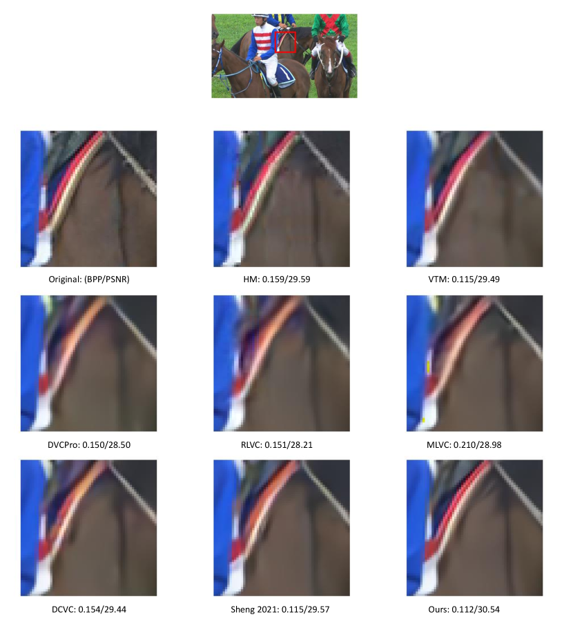
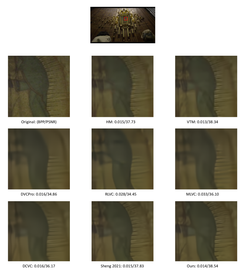
We also conduct the visual comparisons with the previous SOTA neural and traditional video codecs. Two examples are shown in Fig. 17 and Fig. 18. From these comparisons, we can find that our codec can achieve much higher reconstruction quality without increasing the bitrate cost. For instance, in the example shown in Fig. 17, we can find that the frames reconstructed by previous neural codecs have obvious color distortion. By contrast, our codec can restore more accurate stripe color. In Fig. 18, our codec can generate clearer texture details.
Appendix F Other Details
Our codec is built upon previous developments DCVC (Li et al., 2021) and its improved work Sheng 2021 (Sheng et al., 2021). When compared with Sheng 2021 (Sheng et al., 2021), the motion estimation, motion vector encoder/decoder, temporal context mining, and contextual encoder/decoder are reused. The entropy model, quantization mechanism, and frame generator are redesigned. In addition, we add more details on our quantizer and MEMC (motion estimation and motion compensation) process, respectively.
Quantizer. The quantizer works as follows:
-
•
First, the latent representation is divided by the quantization step (QS).
-
•
Second, the mean value is subtracted.
-
•
Third, the latent representation is rounded to the nearest integer and converted into bit-stream via the arithmetic encoder.
During the decoding, the rounded latent representation is first decoded by the arithmetic decoder and adds back the mean value. At last, the QS is multiplied. In this process, most existing image and video codecs use the fixed QS, i.e., 1. By contrast, we decide the QS at multi-granularity levels. First, the global QS is set by the user for the specific target rate. Then it is scaled by the channel-wise QS because different channels contain information with different importance. At last, the spatial-channel-wise QS generated by our entropy model is applied. This can help our codec cope with various video contents and achieve precise rate adjustment at each position.
Motion estimation and motion compensation. The MEMC process can be divided into the following steps:
-
•
First, the original motion vector (MV) between the current frame and the reference frame is estimated via the optical flow estimation network. The MV is dense at full resolution.
-
•
The original MV is then transformed into latent representation via the MV encoder.
-
•
The latent representation of MV is quantized and converted into bit-stream. The quantization step therein is also determined at multi-granularity levels. The quantization and entropy model are similar with those of the latent representation of the current frame.
-
•
The MV at full resolution is then reconstructed via arithmetic decoder and MV decoder.
-
•
The reconstructed MV is used to warp the feature and extract the context via the temporal context mining module.