Hyperbolic Self-supervised Contrastive Learning Based Network Anomaly Detection

Yuanjun Shi Tianjin University switchsyj@tju.edu.cn

Abstract

Anomaly detection on the attributed network has recently received increasing attention in many research fields, such as cybernetic anomaly detection and financial fraud detection. With the wide application of deep learning on graph representations, existing approaches choose to apply euclidean graph encoders as their backbone, which may lose important hierarchical information, especially in complex networks. To tackle this problem, we propose an efficient anomaly detection framework using hyperbolic self-supervised contrastive learning. Specifically, we first conduct the data augmentation by performing subgraph sampling. Then we utilize the hierarchical information in hyperbolic space through exponential mapping and logarithmic mapping and obtain the anomaly score by subtracting scores of the positive pairs from the negative pairs via a discriminating process. Finally, extensive experiments on four real-world datasets demonstrate that our approach performs superior over representative baseline approaches.

1 Introduction

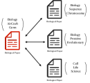
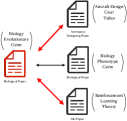
Anomaly detection on attributed networks has received enormous attention. Anomaly detection Li et al. (2019); Ding et al. (2019) refers to the process of spotting data instances that deviate significantly from the majorities. Since the attributed graph is made up of attribute features and edges, in general, there are two types of anomalies, i.e. the attributed anomaly shown in Figure 1(a) and the structural anomaly shown in Figure 1(b). As a result, due to its complexity, it seems difficult to apply a simple anomaly detection method, which is initially employed for attribute-only data Chen et al. (2001) or static plain networks Duan et al. (2020). Furthermore, accessing the ground-truth label in a corrupted attributed graph is expensive. Hence, it is difficult to identify abnormalities in an attributed network immediately due to a lack of appropriate supervision signals. Hence, the key to addressing this issue is to conclude the patterns of normal nodes or abnormal nodes in diverse patterns, and utilize the information from the corrupted network without much supervision signals.

(a) Attribute Anomaly

(b) Structural Anomaly

Figure 1: (a) For the attribute anomaly in a citation network, the red anomaly paper is perturbed with its word attributes. (b) For the structural anomaly, the anomalous citation relationships are indicated by the red edges.

Several approaches have been made to deal with anomaly detection for attributed networks. Some are shallow learning methods, including Perozzi and Akoglu (2016); Li et al. (2017); Peng et al. (2018); Xu et al. (2007). Unfortunately, shallow models are limited by their ability to capture specific patterns due to data sparsity or complex modality issues Ding et al. (2019). For example, Xu et al. (2007) mainly focuses on graph node attributes or topological structures. Perozzi and Akoglu (2016) takes both into account, but only considers its neighbors rather than the node itself.

Moreover, with the development of graph deep learning techniques, graph neural network(GNN) becomes a powerful tool for graph modeling, exhibiting superior performance in a variety applications. For example, Kipf and Welling (2017) proposes graph convolution network by applying the convolutional operation on graph data. Veličković et al. (2018) employs the attention mechanism on graph, which is more competitive in specific inductive tasks. Specifically, some approaches for anomaly detection try to learn feature representation of normality using graph encoders in a generative paradigm, including Li et al. (2019); Ding et al. (2019); Fan et al. (2020). The assumption for this is that normal instances are more likely to be better reconstructed than abnormal ones Pang et al. (2021). However, first, this reconstruction process aims to data compressing rather than anomaly detection, which is designed to learn the general representation of the underlying normal instances. Second, it takes great cost in the computation of reconstruction process when the network is large, as graph convolution operation for the whole graph is required (e.g. SpecAE Li et al. (2019)).

Self-supervised contrastive learning is a feasible alternative for overcoming the aforementioned limitations. Contrastive learning has shown its great potential in many application fields, including computer vision Chen et al. (2020); He et al. (2020), natural language processing Gao et al. (2021) and graph representation learning Zhu et al. (2020, 2021); Hassani and Khasahmadi (2020). It is intended to optimize contrastive loss in order to learn the generic representation of different types of instances. Specifically, similar positive pairs are pulled together, while dissimilar negative ones are pushed apart.

Inspired by Liu et al. (2021), there is consistency between a normal node and its neighbors. While for an abnormal node, there is inconsistency with neighbors in its attributes, graph topologies, or both. Furthermore, the prediction score of the contrastive discriminator is utilized to calculate contrastive loss, which is highly related to alignment and uniformity between different pairs. In this view, contrastive learning is inherently helpful to solve anomaly detection tasks by aligning nodes with their neighbors, where abnormal nodes fail to follow this pattern. Despite their effectiveness, recent work Wilson et al. (2014) has demonstrated that graph data shows more hyperbolic geometric properties, as the number of nodes rises exponentially with the growth of distance to the root of the whole graph. Intuitively, complex networks with hierarchical information can be naturally embedded into hyperbolic space. Recent approaches Liu et al. (2019); Chami et al. (2019); Zhang et al. (2021) have exhibited great modeling ability of hyperbolic graph neural networks on attributed graphs, resulting in great improvements on several node classification tasks.

In view of this, we extend the contrastive learning method to the hyperbolic space via the self-supervised learning paradigm to utilize the hierarchical relationship between different nodes and to solve accompanying challenges: (1) how to sample positive and negative pairs, which are subsequently encoded into the hyperboloid model making use of hierarchical information; (2) how to distinguish between positive and negative pairs in the hyperboloid model, which is different from the fundamental contrastive learning framework. The main contributions are summarized as below.

•

Propose an efficient anomaly detection framework using hyperbolic self-supervised contrastive learning. To the best of our knowledge, we are the first to extend contrastive learning to hyperbolic space for anomaly detection utilizing the rich information of hierarchical graph data via exponential mapping and logarithmic mapping.
•

Perform subgraph sampling and target nodes anonymization to conduct data augmentation, and employ discriminator after hyperboloid encoding and tangent space decoding. To demonstrate the notion of the hierarchical information, we further analyze the key role of our hyperboloid encoder and tangent decoder in the ablation study. Furthermore, we also conduct subgraph matrix calculation stably and efficiently.
•

Conduct extensive experiments on four real-world datasets and demonstrate that our approach performs superior over representative baseline approaches. Moreover, results suggest that the more hyperbolic the dataset is, the more improvements this method can make.

2 Related Work

2.0.1 Anomaly Detection on Networks

Traditional non-deep learning anomaly detection techniques, such as AMEN Perozzi and Akoglu (2016) focus on detecting abnormality of subgraphs with node information in an ego-net. Radar Li et al. (2017) learns residual error by reconstruction and considers the top-k nodes with larger norms of error as anomalies. ANOMALOUS Peng et al. (2018) tries to use CUR matrix decomposition to select attributes, which is closely related to network structure, followed by the same residual analysis used in Radar. Although these techniques try to capture graph information from attributes and structures, they cannot work well on large complex networks.

Moreover, graph deep learning techniques have been applied in varieties of applications. DOMINANT Ding et al. (2019) aims to minimize network and attribute reconstruction errors with node representations embedded by a graph convolutional encoder. SpecAE Li et al. (2019) applies graph convolutional encoder to learn nodes representations and detect anomalies through a density estimation approach. Unfortunately, reconstruction-based methods also have disadvantages: the training object is reconstruction error instead of anomaly score itself, which results in overfitting to the general patterns of normal nodes. Hence, it cannot handle the out-of-distribution(OOD) problem in inductive tasks.

More recent works combine supervised contrastive learning with anomaly detection. Contrastive learning across different data augmentation views has recently achieved the state-of-the-art in the field of self-supervised learning, aiming to learn representations by pulling similar pairs closer and pushing dissimilar ones away. Such as CoLA Liu et al. (2021) uses the “target node v.s local subgraph” view. ANEMONE Jin et al. (2021) proposes a multi-view contrastive learning method, which employs not only “node v.s neighbor” but also “node v.s node”. Despite their success, it is not an appropriate way to model large complex networks, which contains rich hierarchical information.

2.0.2 Hyperbolic Graph Neural Network

Recently, Hyperbolic Graph Neural Networks (HGNNs Liu et al. (2019)) has attracted more attention. Different from GCN Kipf and Welling (2017) and GAT Veličković et al. (2018), HGNNs are designed for modeling complex networks with higher ordered hierarchical information Wilson et al. (2014). HGCN Chami et al. (2019) defines convolution operation and neighborhood aggregation in hyperbolic space, whereas HAT Zhang et al. (2021) proposed a graph attention mechanism in hyperbolic space. And these hyperbolic models have shown great improvements on graph modeling tasks. To tackle the problem mentioned above, in this paper, we apply contrastive learning method for anomaly detection in the hyperbolic space while paying extra attention to the hierarchical information between nodes.

3 Proposed Method

Refer to caption — Figure 2: Our model framework: we first perform subgraph sampling and target nodes anonymization from the real-world attributed network containing anomalies as Graph Data Augmentation step, and then apply Hyperbolic Mapping through exponential mapping and logarithmic mapping. Finally, we can get anomaly score by subtracting scores of the positive pairs from the negative pairs via the Discriminating Process. Specifically, we should note that red nodes denote the anomalies while blue nodes denote the normal ones in the attributed network.

3.1 Preliminaries: Hyperbolic Geometry

Riemannian Manifold.

A manifold $\mathcal{M}$ is a topological space mapping from the original space $\mathbb{R}^{d}$ near each point, referring to a generalization of surfaces in high dimensions. Intuitively, for each $x\in\mathcal{M}$ , there is a tangent space $\mathcal{T}_{\mathbf{x}}\mathcal{M}$ of the same dimension as $\mathcal{M}$ , including all possible directions of curves in $\mathcal{M}$ passing through $\mathbf{x}$ .

For a smooth manifold $\mathcal{M}$ , a Riemannian manifold is defined as a pair ( $\mathcal{M},\textbf{g}$ ), where $\textbf{g}=(g_{\mathbf{x}})_{\mathbf{x}\in\mathcal{M}}$ is a Riemannian metric measuring the distance on $\mathcal{M}$ , and $g_{\mathbf{x}}:\mathcal{T}_{\mathbf{x}}\mathcal{M}\times\mathcal{T}_{\mathbf{x}}\mathcal{M}\to\mathbb{R}$ . We can use exponential and logarithmic methods to map between Riemannian manifold and its tangent space. For a certain point $\mathbf{x}\in\mathcal{T}_{\mathbf{x}}\mathcal{M}$ , the exponential mapping: $exp_{\mathbf{x}}(\mathbf{u})$ projects the vector from tangent space to Riemannian manifold. While the logarithmic mapping: $log_{\mathbf{x}}(\mathbf{v})$ projects the vector to its tangent space. For two given points $\mathbf{x},\mathbf{y}\in\mathcal{M}$ , the parallel transport $P_{\mathbf{x}\to\mathbf{y}}(\mathbf{u})$ maps a vector $\mathbf{u}\in\mathcal{T}_{\mathbf{x}}\mathcal{M}$ to $\mathcal{T}_{\mathbf{y}}\mathcal{M}$ .

Hyperbolic Space.

The hyperbolic space is a connected Riemannian manifold with negative curvature. There are several hyperbolic models, such as Poincaré or Hyperboloid model (a.k.a the Minkowski or Lorentz model). We will give the detailed information about hyperboloid model utilized for further discussion.

Given two vectors $\mathbf{u},\mathbf{v}$ in the tangent space $\mathcal{T}_{\mathbf{x}}\mathbb{H}_{d}^{K}=\{\mathbf{y}\in\mathbb{R}^{d+1}|\langle\mathbf{x},\mathbf{y}\rangle_{\mathcal{L}}=0\}$ , we denote the hyperboloid metric $\mathbf{g}_{\mathbf{x}}^{K}(\mathbf{u},\mathbf{v})=\langle\mathbf{u},\mathbf{v}\rangle_{\mathcal{L}}$ , where $\langle{\cdot,\cdot}\rangle_{L}:\mathbb{R}^{d+1}\times\mathbb{R}^{d+1}\to\mathbb{R}$ denotes the Minkowski inner product:

\langle\mathbf{x},\mathbf{y}\rangle_{\mathcal{L}}=-x_{0}y_{0}+x_{1}y_{1}+...+x_{d}y_{d}.

(1)

Hence, the hyperboloid model $\mathbb{H}$ with a negative curvature $-1/K(K>0)$ in $d$ dimensions is defined as:

(\mathbb{H}^{d,K},\textbf{g})=\{\mathbf{x}\in\mathbb{R}^{d+1}:\langle\mathbf{x},\mathbf{x}\rangle_{L}=-K,x_{0}>0\}.

(2)

Furthermore, we can use exponential mapping, logarithmic mapping, and parallel transport equation for mapping between euclidean space and hyperbolic space:

exp_{\mathbf{x}}^{K}(\mathbf{v})=cosh(\frac{\|\mathbf{v}\|_{\mathcal{L}}}{\sqrt{K}})\mathbf{x}+\sqrt{K}sinh({\frac{\|\mathbf{v}\|_{\mathcal{L}}}{\sqrt{K}}})\frac{\mathbf{v}}{\|\mathbf{v}\|_{\mathcal{L}}},

(3)

where $\|\mathbf{v}\|_{\mathcal{L}}=\sqrt{\langle\mathbf{v},\mathbf{v}\rangle_{\mathcal{L}}}$ denotes the norm of $\mathbf{v}$ .

log_{\mathbf{x}}^{K}(\mathbf{v})=d_{\mathcal{L}}^{K}(\mathbf{x},\mathbf{v})\frac{\mathbf{v}+\frac{1}{K}\langle\mathbf{x},\mathbf{v}\rangle_{\mathcal{L}}\mathbf{x}}{\|\mathbf{v}+\frac{1}{K}\langle\mathbf{x},\mathbf{v}\rangle_{\mathcal{L}}\mathbf{x}\|_{\mathcal{L}}},

(4)

where $d_{\mathcal{L}}^{K}(\mathbf{x},\mathbf{v})$ is the distance between two points in $\mathbb{H}_{d}^{K}$ :

d_{\mathcal{L}}^{K}(\mathbf{x},\mathbf{v})=\sqrt{K}arcosh(\frac{-\langle\mathbf{x},\mathbf{v}\rangle_{\mathcal{L}}}{K}).

(5)

Parallel transport in hyperboloid model is used for mapping a vector from one tangent space to another. Concretely, given a vector $\mathbf{v}\in\mathcal{T}_{\mathbf{x}\mathcal{M}}$ , transport $P_{\mathbf{x}\to\mathbf{y}}(\mathbf{v})$ maps $\mathbf{v}$ to a Riemannian tensor in $\mathcal{T}_{\mathbf{y}}\mathcal{M}$ .

3.2 Problem Definition: Anomaly Detection on Attributed Networks

Attributed Network.

Given a node set $\mathcal{V}=(v_{1},...,v_{n})$ , an adjacency matrix $\mathbf{A}\in\mathbb{R}^{n\times n}$ , and an attribute matrix $\mathbf{X}\in\mathbb{R}^{n\times d}$ , an attributed network $\mathcal{G}$ can be defined as $\mathcal{G}=(\mathcal{V},\mathbf{A},\mathbf{X})$ . The $i$ -th row of attribute matrix $\mathbf{X}$ denotes the attribute information of node $v_{i}$ . In the adjacency matrix, $\mathbf{A}_{i,j}=1$ if there is a connection between node $v_{i}$ and $v_{j}$ , otherwise $\mathbf{A}_{i,j}=0$ .

Anomaly Detection on Attributed Network.

Given an attributed network $\mathcal{G}=(\mathcal{V},\mathbf{A},\mathbf{X})$ , our task is to learn a function $f$ to calculate the anomaly score $f(v_{i})$ for each node $v_{i}\in\mathcal{G}$ , according to its attribute information and graph structure. The higher the node’s anomaly score is, the more likely it is to be anomalous.

3.3 Contrastive Learning for Anomaly Detection in Hyperbolic Space

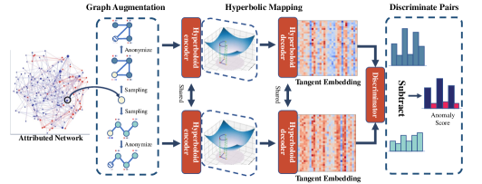
We propose an efficient hyperboloid contrastive learning method for anomaly detection. As shown in Figure 2, our detection pipeline contains four steps: (1) We employ graph data augmentation by sampling positive and negative pairs for each node. (2) The hyperboloid encoder and decoder extract hierarchical embedding in the tangent space for the selected node and its neighbor embedding through a graph readout module. (3) We obtain discriminate score for positive and negative pairs through a discriminator respectively, measuring the agreement between the selected node with different pairs. (4) Finally, we calculate the discriminate scores mentioned above using multiple rounds sampling method, which is more robust to our paradigm. Specifically, it is an overall observation of all surrounding neighbors for each node.

In general, the training object is to discriminate positive pairs and negative pairs in the tangent space, which is highly related to the anomaly detection task, due to the disagreement between anomalous node and its neighbor.

3.3.1 Graph Sampling

The most important step of contrastive learning is data augmentation. Different from contrastive learning method applied in computer vision Chen et al. (2020); He et al. (2020) and natural language processing Gao et al. (2021), graph data augmentation is more complex in specific method and implementation level. Existing graph data augmentation methods such as Zhu et al. (2021); Hassani and Khasahmadi (2020), are mainly employed on nodes and edges at the whole graph level, which is useful for graph embedding learning but unsuitable for anomaly detection, especially in hyperbolic space, which may perturb the hierarchical order. Inspired by CoLA Liu et al. (2021), an abnormal node usually shows more inconsistency with its neighbors in anomaly detection task. The heuristic is that a normal node is more consistent with its immediate neighbor than other non-neighbor nodes, but abnormal nodes never are. Thus, we extend a sampling method to hyperbolic space preserving its local hierarchical structure for anomaly detection.

Concretely, our designation focuses on the consistency of the node and its local neighbors in the tangent space via a “target node v.s. neighbor subgraph” paradigm. As is shown in Figure 2, first, a target node is randomly selected from the whole graph. Second, its neighbor is denoted as the node set by adopting RWR algorithm Tong et al. (2006) in the tangent space. For a node $v_{i}$ , a positive pair $P_{i}^{+}=\{v|v\in Neighbor(v_{i})\}$ is the neighbor of $v$ , and a negative pair $P_{i}^{-}=\{v|v\notin Neighbor(v_{i})\}$ is randomly chosen from the neighbor of other nodes. To prevent contrastive learning method from recognizing such patterns easily, we also anonymize target node in the sampled pairs. Specifically, we mask the attribute vector of the target node.

Overall, we implement the graph traversal algorithm to sample for each point in the whole graph.

3.3.2 Hyperboloid Transformation

After the graph sample step, instance pairs (either positive or negative) are denoted as $\mathcal{P}=(P^{+}_{1},...,P^{+}_{n},P^{-}_{1},...,P^{-}_{n})$ , and $n$ is the number of nodes. For each instance pair $P_{i}=(v_{i},\mathcal{S}_{i},y_{i})$ , where $v_{i}$ is the selected target node, $\mathcal{S}_{i}=(A_{i},X_{i})$ is the subgraph generated from random walk with restart algorithm with node $v_{i}$ , where $A_{i}$ denotes subgraph adjacency matrix, and $X_{i}$ denotes subgraph attribute matrix. $y_{i}$ denotes the node anomaly label, and is defined as: if $v_{i}\text{ is abnormal}$ , then $y_{i}=1$ ; otherwise, $y_{i}=0$ .

To utilize the rich hierarchical information in attributed graph, we first map the attribute of node $v_{i}$ and nodes in subgraph $\mathcal{S}_{i}=$ from the tangent space to hyperbolic space at the origin point by an exponential mapping. For each node $v\in\{v_{i}\cup\mathcal{S}_{i}\}$ , and its attribute $x$ :

\begin{split}x^{H}&=exp_{\mathbf{o}}^{K}((0,x^{E})),\\ &=(\sqrt{K}cosh(\frac{\|x^{E}\|_{2}}{\sqrt{K}})\sqrt{K}sinh(\frac{\|x^{E}\|_{2}}{\sqrt{K}})\frac{x^{E}}{\|x^{E}\|_{2}}),\end{split}

(6)

where $(0,x^{E})\in\mathbb{R}^{d+1}$ is considered as a point in $\mathcal{T}_{\mathbf{o}}\mathbb{H}^{d,K}$ , and $\mathbf{o}$ denotes the origin point in $\mathbb{H}^{d,K}$ . Recall that $\langle(0,x^{E}),\mathbf{o}\rangle=0$ , where we use $\mathbf{o}=(\sqrt{K},0,...,0)\in H^{d,K}$ as a reference point to perform tangent space operations.

For each $\mathcal{S}_{i}$ , we apply graph convolution module to aggregate its local information in the subgraph and embed hierarchical information for each node simultaneously. A single layer $l$ with a learning curvature $K$ of hyperbolic hraph convolution can be written as:

$\displaystyle H_{i}^{l}$	$\displaystyle=(W^{l-1}\otimes^{K_{l-1}}H_{i}^{l-1})\oplus^{K_{l-1}}b^{l-1},$	(7)
$\displaystyle AGG_{i}^{l}$	$\displaystyle=Aggregate^{K_{l-1}}(log_{\mathbf{o}}^{K_{l-1}}(H_{i}^{l-1}),Adj_{i}),$	(8)
$\displaystyle Act_{i}^{l}$	$\displaystyle=\sigma^{K_{l,l-1}}(AGG_{i}^{l}),$	(9)

where $H_{i}^{l-1}$ and $H_{i}^{l}$ $\in\mathbb{R}^{(subgraph\_size,d)}$ are the hidden subgraph representations of layer $l-1$ and layer $l$ , $W_{l}$ and $b^{l}$ are the learning parameters, $Adj_{i}$ denotes the normalized adjacency matrix $\widetilde{D_{i}}^{-\frac{1}{2}}\widetilde{(A_{i}+I)}\widetilde{D_{i}}^{-\frac{1}{2}}$ . For $l=0$ , $H_{i}^{0}=X_{i}^{H}$ is the subgraph attributed matrix in hyperbolic space. Operator $\otimes^{K_{l-1}}$ represents hyperbolic matrix multiplication, which can be computed through the logarithmic mapping followed by the exponential mapping:

W^{l}\otimes^{K_{l-1}}H^{l-1}=exp_{\mathbf{o}}^{K_{l-1}}(Wlog_{\mathbf{o}}^{K_{l-1}}H^{l-1}).

(10)

The same as $\otimes^{K_{l-1}}$ , $\oplus^{K_{l-1}}$ is mobius add in hyperbolic space with curvature $K_{l-1}$ , can be computed through the parallel transport:

H^{l-1}\oplus^{K_{l-1}}b^{l-1}=exp_{H^{l-1}}^{K_{l-1}}(P_{\mathbf{o}\to H^{l-1}}^{K_{l-1}}(b)).

(11)

In detail, we implement the ReLU function as non-linear activation function in equation (9).

3.3.3 Anomaly Discriminator

The discriminator aims to distinguish between positive and negative pairs for a selected node and its local subgraphs. Specifically, we first decode the node representation to the tangent sapce and then project it into classification space. Furthermore, we apply $bilinear$ function to compute the similarity score between a selected node and its subgraph instance pairs via a graph readout module.

H_{i}^{E}=W\times log_{\mathbf{o}}^{K}(H_{i}^{H})+b,

(12)

s_{i}=Readout(H_{i}^{E})=\frac{1}{n}\sum_{k=0}^{n}h_{k}^{E},

(13)

where $n$ is the number of nodes in a subgraph. We can get the node representation for $v_{i}$ with the same hyperboloid encoder and decoder for the following score computation:

q_{i}=Bilinear(DEC(ENC(X_{(v_{i})})),s_{i}),

(14)

where the ENC denotes the convolutional encoder in our hyperboloid model mentioned above and the DEC denotes the parallel transportation from the hyperbolic space to the tangent space at the origin point. It is worth mentioning that we also apply different kinds of discriminate methods, including contrasting positive and negative pairs in hyperbolic space directly and attention-based readout module. But we do not observe any improvement. Detailed results are discussed in the Ablation Study, where conducting w/o hyperboloid decoder denotes discriminate directly in the hyperbolic space.

3.3.4 Loss Function

After discriminate score computation, our contrastive learning objective can be viewed as the binary classification task. The learning process is to discriminate between target node and positive or negative pairs. The same as label $y_{i}$ , for a positive pair the predicted label is expected to be $1$ , while for negative one is expected to be $0$ . Hence, we adopt binary cross-entropy (BCE) loss as our criterion function. Given a batch of training instances $\mathcal{P}=\{\mathcal{P}_{1},...,\mathcal{P}_{N}\}$ , our criterion function can be computed as:

\mathcal{L}=-\sum_{i=1}^{N}y_{i}log(q_{i})+(1-y_{i})log(1-q_{i}).

(15)

3.3.5 Anomaly Detection

In the final step, we can get anomaly score by making subtraction between the score of a positive pair $\mathcal{P}_{i}^{+}$ and a negative pair $\mathcal{P}_{i}^{-}$ , since a normal node is consistent with its neighbor in a positive pair, while exhibits more inconsistency with a negative pair. For a normal node, the discriminate score of a positive pair is closer to 1, while for a negative pair is closer to 0. In contrast, for a abnormal node, there is small margin of discriminate score between a positive and negative pair, because the model fails to generalize such pattern via training on a large amount of normal node. Hence, the anomaly score can be computed as:

Q_{i}=q_{i}^{-}-q_{i}^{+}.

(16)

Concretely, for further robustness of our hyperboloid model, we sample $R$ rounds for each node, obtaining an overall view. On the other hand, for a structural anomaly node which contains some uncorrelated edges in the subgraph is more difficult to capture its abnormality through few rounds detection. Thus, we implement the multi-round neighbor detection, which can be computed as:

	$\displaystyle Q_{(i,R)}$	$\displaystyle=q_{(i,r)}^{-}-q_{(i,R)}^{+},$		(17)
	$\displaystyle Q_{i}$	$\displaystyle=\frac{1}{R}\sum_{k=0}^{R}Q_{(i,R)},$		(18)

where $q_{(i,R)}$ denotes the discriminate score of node $v_{i}$ either a positive or negative instance pair.

3.3.6 Time Complexity Analysis

We further analyze the time complexity of our framework with main steps aforementioned in section 3.3. Specifically, we apply random walk with restart (RWR) algorithm to sample positive and negative pairs, the time complexity for batch size $n$ with local subgraph size $c$ and mean degree $\sigma$ is $\mathcal{O}(nc\sigma)$ . In the hyperboloid encoder, we perform hyperboloid linear transformation, local aggregation and non-linear activation, which costs $\mathcal{O}(nkc^{2})$ , where $k$ denotes the hidden size. In the hyperboloid decoder, we employ tangent space projection, which costs $\mathcal{O}(nc)$ . Furthermore, the discriminator for each instance costs $\mathcal{O}(2nk)$ . Finally, the overall time complexity is $\mathcal{O}(n(c\sigma+kc^{2}+c+2k))$ .

4 Experiments

Datesets. To evaluate our proposed hyperboloid model, we test the performance on four widely used datasets, including three social networks and a flight network. The statistics of the datasets are listed in Table 1. We report Gromov’s $\sigma$ hyperbolicity values to indicate its hyperbolic geometry, where the lower $\sigma$ is, the more hyperbolic the dataset should be.

•

Citation Networks. CORA, CITESEER and PUBMED are public citation network datasets. Nodes represent scientific papers and edges represent citation relations. The attribute feature is the bag of word representation, where dimension is determined by its dictionary size.
•

Flight Networks. We follow the same settings in HGCN Chami et al. (2019). The nodes in airport denote the airports, and edges indicate flights. The attributes indicate the geographic information including longitude, latitude, altitude and GDP.

Following previous works Ding et al. (2019); Liu et al. (2021), we inject a combination of structural anomalies and attribute anomalies into each dataset since there are no ground-truth anomalies in these datasets mentioned above. Concretely, the attribute anomalies are constructed by adding extra noise to $k$ selected nodes. For node $v_{i}$ , we first randomly select adequate number of nodes as candidates, and choose the least similar node $v_{j}$ to change the attribute of $v_{i}$ as $v_{j}$ , according to the euclidean distance between two nodes. The structural anomalies are constructed by adding extra noise to the topological structure of the network. We first choose $n$ cliques that contains $m$ nodes each as fully connected graphs. To balance the number of two types of anomalies, we set $k=p\times q$ , according to the number of nodes in each dataset. Specifically, following the settings in previous works, we set $p=15$ for all datasets, and $q=5,5,20,5$ for CORA, CITESEER, PUBMED, and AIRPORT.

Dataset	Nodes	Edges	Features	Anomaly	$\sigma$
CORA	2708	5429	1433	0.06	2.5
CITESEER	3327	4732	3703	0.05	4.0
PUBMED	19717	44338	500	0.03	2.5
AIRPORT	3188	18631	1000	0.05	1.5

Table 1: Statistics of datasets.

Baselines. For comparison, we choose different baseline models, including naive and localized (especially for anomaly detection task) contrastive learning models, and original hyperboloid models used for classification task. Since shallow based methods cannot achieve satisfactory performance limited by their intrinsic mechanism which cannot cope with complex network structure and sparse attributes, we do not make further comparison with these methods. (1) DOMINANT. Ding et al. (2019) DOMINANT is a reconstruction based method. It aims at reconstructing the adjacency matrix and the attribute matrix after employing graph convolution network. For inference step, it utilizes ranking strategy by choosing nodes with higher reconstruction error as anomalies. (2) MVGRL. Hassani and Khasahmadi (2020) MVGRL is a graph contrastive learning method for representation learning. It generates graph embedding by contrasting in “node v.s node” and “graph v.s graph” views simultaneously. The bilinear function is used to discriminate between positive and negative sample pairs. (3) CoLA. Liu et al. (2021) CoLA is a contrastive learning method framework for anomaly detection task in euclidean space. It utilizes the general “node v.s neighbor” paradigm but the hierarchical information is ignored in this process. For AIRPORT dataset, we take the same hidden dimension setting used in our model, and then take an average metric on different ten seeds. Concretely, we set $lr=0.001$ and $hidden\_dim=64$ and run $100$ epochs for training. (4) HGCN. Chami et al. (2019) HGCN is the Hyperboloid Graph Convolutional Network, which is designed for graph embedding tasks via supervised learning. Here, we employ the same train/val/test split method as Chami et al. (2019). For AIRPORT, we set the train/val/test set proportion as $0.15/0.15/0.7$ respectively.

Hyperparameter Settings. For all datasets, the learning rate is set as $0.03$ . We apply Adam optimizer with $0.999$ momentum, and $0.0001$ weight decay value for CITESEER, PUBMED and AIRPORT, $0.0002$ for CORA. We should note that we also apply Riemannian Adam optimizer, but it fails to converge in this situation. Dropout is the key to prevent the model from overfitting for a certain dataset. We set dropout rate to 0.5 for CORA and 0.1 for CITESEER, PUBMED and AIRPORT. We should note that we set curvature $K=2.5$ for CORA, PUBMED and AIRPORT, $K=1.0$ for CITESEER. In the inference stage, we perform $256$ rounds detection method to get an overall view of a target node.

Anomaly Detection Results and Analysis. We evaluate the performance of our model on four datasets compared with three baseline models in Table 2. Concretely, we employ the ROC-AUC metric, where ROC is the curve of true positive rate against false positive rate. AUC is the value of ROC curve under area, which demonstrates how confident our model is to make the right predictions. When the AUC value is closer to 1, it means the model has a better performance.

Methods		CORA	CITESEER	PUBMED	AIRPORT
Hyperbolicity		$\mathbf{\sigma}$ =2.5	$\mathbf{\sigma}$ =4.0	$\mathbf{\sigma}$ =2.5	$\mathbf{\sigma}$ =1.5
Euclidean	DOMINANT	0.8155	0.8251	0.8081	0.6964
	MVGRL	0.6255	0.4096	0.6714	0.4604
	CoLA	0.8827	0.8968	0.9512	0.7575
Hyperboloid	HGCN	0.5285	0.6984	0.5966	0.6221
Hyperboloid	Ours	0.8914	0.7618	0.9513	0.7805

Table 2: AUC results of our proposed approach and baselines.

The average results are exhibited in Table 2, where we experiment on five seeds. Compared with the baselines, our model improves 5.42% using the AUC score on AIRPORT dataset, which has the lowest hyperbolicity value. Overall, we can get the following observations. Our model shows significant performance on AIRPORT dataset, which has a lower hyperbolicity value. Generally, the more hyperbolic the dataset is, the better performance it can obtain.

Ablation	AIRPORT	PUBMED	CORA	Avg.
w/o hyperboloid decoder	0.7273	0.9386	0.8097	0.8252
w/o hyperbolic space	0.7590	0.9160	0.6464	0.7738
Full model	0.7805	0.9513	0.8914	0.8744

Table 3: AUC results of ablation study on the different datasets.

The Ablation Study. To illustrate the role of encoder and decoder of our hyperboloid contrastive learning model, we perform an ablation study on the AIRPORT, PUBMED and CORA datasets, where we outperform the baseline approaches. As shown in Table 3, compared to employing contrastive learning model directly in the hyperbolic space without a logarithmic mapping decoder, the AUC score decreases by 4.92%. Furthermore, we explore the role of our hyperboloid model by discriminating positive and negative pairs in the euclidean space. The AUC score decreases by 10.06%.

Case Study. We conduct a case study on the AIRPORT dataset to make a detailed comparison with the Euclidean-based model CoLA Liu et al. (2021). As shown in Figure 3, P610 has two anomaly neighbors P1361 and P2632(due to the space limitation, we only show two of its neighbors). In comparison to the baseline model, our hyperboloid model can more efficiently detect anomalies utilizing the hierarchical information. Table 4 shows that our model predicts anomalies with a small margin computed by equation(16). The smaller the margin is, the more likely it is an anomaly node. Hence, we can imply that our model is much easier to distinguish anomalies from the normal ones than the baseline with the same 32 hidden neurons setting.

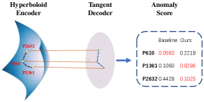
Methods	Point	Negative( $q_{i}^{-}$ )	Positive( $q_{i}^{+}$ )	Margin= $\|q_{i}^{-}-q_{i}^{+}\|$
CoLA	P610	0.2285	0.2868	0.0583
	P1361	0.2739	0.1679	0.1060
	P2632	0.2805	0.7233	0.4428
Ours	P610	0.1901	0.4119	0.2218
	P1361	0.2156	0.2442	0.0286
	P2632	0.1631	0.2656	0.1025

Table 4: Results of P160 and its neighbor in the AIRPORT dataset, where the margin denotes the anomaly score.

5 Conclusion

In this paper, we propose the anomaly detection framework based on hyperbolic self-supervised contrastive learning. We are the first to introduce the contrastive learning method to the hyperbolic space, especially for the anomaly detection task. In our hyperboloid model, hierarchical information is included via exponential and logarithmic mapping. Results show that the more hyperbolic the dataset is, the more hierarchical information it can obtain. Furthermore, we conduct an ablation study to illustrate the key role of hyperboloid encoder and decoder. In comparison to baselines, our approach detects anomalies in a small margin, implying that our model is more confident in the detection results. We hope that our work will inspire future work on hyperbolic graph learning.

References

Chami et al. [2019] Ines Chami, Zhitao Ying, Christopher Ré, and Jure Leskovec. Hyperbolic graph convolutional neural networks. Advances in neural information processing systems, 32:4868–4879, 2019.
Chen et al. [2001] Yunqiang Chen, Xiang Sean Zhou, and Thomas S Huang. One-class svm for learning in image retrieval. In Proceedings 2001 International Conference on Image Processing, volume 1, pages 34–37. IEEE, 2001.
Chen et al. [2020] Ting Chen, Simon Kornblith, Mohammad Norouzi, and Geoffrey Hinton. A simple framework for contrastive learning of visual representations. In ICML, pages 1597–1607. PMLR, 2020.
Ding et al. [2019] Kaize Ding, Jundong Li, Rohit Bhanushali, and Huan Liu. Deep anomaly detection on attributed networks. In Proceedings of the 2019 SIAM International Conference on Data Mining, pages 594–602. SIAM, 2019.
Duan et al. [2020] Dongsheng Duan, Lingling Tong, Yangxi Li, Jie Lu, Lei Shi, and Cheng Zhang. Aane: Anomaly aware network embedding for anomalous link detection. In 2020 IEEE International Conference on Data Mining (ICDM), pages 1002–1007. IEEE, 2020.
Fan et al. [2020] Haoyi Fan, Fengbin Zhang, and Zuoyong Li. Anomalydae: Dual autoencoder for anomaly detection on attributed networks. In ICASSP 2020-2020 IEEE International Conference on Acoustics, Speech and Signal Processing (ICASSP), pages 5685–5689. IEEE, 2020.
Gao et al. [2021] Tianyu Gao, Xingcheng Yao, and Danqi Chen. SimCSE: Simple contrastive learning of sentence embeddings. In EMNLP, 2021.
Hassani and Khasahmadi [2020] Kaveh Hassani and Amir Hosein Khasahmadi. Contrastive multi-view representation learning on graphs. In Proceedings of International Conference on Machine Learning, pages 3451–3461. 2020.
He et al. [2020] Kaiming He, Haoqi Fan, Yuxin Wu, Saining Xie, and Ross Girshick. Momentum contrast for unsupervised visual representation learning. In Proceedings of the IEEE/CVF Conference on Computer Vision and Pattern Recognition, pages 9729–9738, 2020.
Jin et al. [2021] Ming Jin, Yixin Liu, Yu Zheng, Lianhua Chi, Yuan-Fang Li, and Shirui Pan. Anemone: Graph anomaly detection with multi-scale contrastive learning. In Proceedings of the 30th ACM International Conference on Information & Knowledge Management, pages 3122–3126, 2021.
Kipf and Welling [2017] Thomas N. Kipf and Max Welling. Semi-supervised classification with graph convolutional networks. In ICLR, 2017.
Li et al. [2017] Jundong Li, Harsh Dani, Xia Hu, and Huan Liu. Radar: Residual analysis for anomaly detection in attributed networks. In IJCAI, pages 2152–2158, 2017.
Li et al. [2019] Yuening Li, Xiao Huang, Jundong Li, Mengnan Du, and Na Zou. Specae: Spectral autoencoder for anomaly detection in attributed networks. In Proceedings of the 28th ACM International Conference on Information and Knowledge Management, pages 2233–2236, 2019.
Liu et al. [2019] Qi Liu, Maximilian Nickel, and Douwe Kiela. Hyperbolic graph neural networks. CoRR, abs/1910.12892, 2019.
Liu et al. [2021] Yixin Liu, Zhao Li, Shirui Pan, Chen Gong, Chuan Zhou, and George Karypis. Anomaly detection on attributed networks via contrastive self-supervised learning. IEEE Transactions on Neural Networks and Learning Systems, 2021.
Pang et al. [2021] Guansong Pang, Chunhua Shen, Longbing Cao, and Anton Van Den Hengel. Deep learning for anomaly detection: A review. ACM Computing Surveys (CSUR), 54(2):1–38, 2021.
Peng et al. [2018] Zhen Peng, Minnan Luo, Jundong Li, Huan Liu, and Qinghua Zheng. Anomalous: A joint modeling approach for anomaly detection on attributed networks. In IJCAI, pages 3513–3519, 2018.
Perozzi and Akoglu [2016] Bryan Perozzi and Leman Akoglu. Scalable anomaly ranking of attributed neighborhoods. In Proceedings of the 2016 SIAM International Conference on Data Mining, pages 207–215. SIAM, 2016.
Tong et al. [2006] Hanghang Tong, Christos Faloutsos, and Jia-Yu Pan. Fast random walk with restart and its applications. In ICDM), pages 613–622. IEEE, 2006.
Veličković et al. [2018] Petar Veličković, Guillem Cucurull, Arantxa Casanova, Adriana Romero, Pietro Liò, and Yoshua Bengio. Graph Attention Networks. International Conference on Learning Representations, 2018. accepted as poster.
Wilson et al. [2014] Richard C Wilson, Edwin R Hancock, Elżbieta Pekalska, and Robert PW Duin. Spherical and hyperbolic embeddings of data. IEEE transactions on pattern analysis and machine intelligence, 36(11):2255–2269, 2014.
Xu et al. [2007] Xiaowei Xu, Nurcan Yuruk, Zhidan Feng, and Thomas AJ Schweiger. Scan: a structural clustering algorithm for networks. In Proceedings of the 13th ACM SIGKDD international conference on Knowledge discovery and data mining, pages 824–833, 2007.
Zhang et al. [2021] Yiding Zhang, Xiao Wang, Chuan Shi, Xunqiang Jiang, and Yanfang Fanny Ye. Hyperbolic graph attention network. IEEE Transactions on Big Data, 2021.
Zhu et al. [2020] Yanqiao Zhu, Yichen Xu, Feng Yu, Qiang Liu, Shu Wu, and Liang Wang. Deep Graph Contrastive Representation Learning. In ICML Workshop on Graph Representation Learning and Beyond, 2020.
Zhu et al. [2021] Yanqiao Zhu, Yichen Xu, Feng Yu, Qiang Liu, Shu Wu, and Liang Wang. Graph contrastive learning with adaptive augmentation. In Proceedings of the Web Conference 2021, pages 2069–2080, 2021.