Hyperbolic volume and Heegaard distance
Abstract.
We prove (Theorem 1.5) that there exists a constant so that if is a -generic complete hyperbolic 3-manifold of volume and is a Heegaard surface of genus , then , where denotes the distance of as defined by Hempel. The term -generic is described precisely in Definition 1.3; see also Remark 1.4.
The key for the proof of Theorem 1.5 is Theorem 1.8 which is on independent interest. There we prove that if is a compact 3-manifold that can be triangulated using at most tetrahedra (possibly with missing or truncated vertices), and is a Heegaard surface for with , then .
Key words and phrases:
3-manifold, Heegaard splittings, Heegaard distance1991 Mathematics Subject Classification:
57M99, 57M251. Introduction
All the manifolds considered in this paper are 3-dimensional, compact, connected, and orientable. By hyperbolic manifold we mean a manifold whose interior admits a complete finite volume Riemannian metric locally isometric to hyperbolic 3-space .
It is generally agreed that the volume of a hyperbolic manifold , , is a good measure of the complexity of . As evidence of that, arguments of M. Gromov, T. Jørgensen and W. Thurston show that the hyperbolic volume is linearly equivalent to the number of tetrahedra needed to triangulate a link exterior in . The argument is based on Thurston’s notes [thurston], for a detailed presentation see [gjt]; throughout this paper we follow the notation and definitions given in that paper. For a precise statement, let be the smallest number of tetrahedra needed to triangulate , where the minimum is taken over all links (possibly, ) and all possible triangulations.
Theorem 1.1 (Gromov, Jørgensen, Thurston).
There exist constants so that for any hyperbolic manifold the following holds:
Remark 1.2.
In the proof of Theorem 1.1 given in [gjt] it is shown that given , a Margulis constant for , and , there exists , so that can be triangulated using at most tetrahedra; here denotes the closed -neighborhood of the -thick part of . We note that depends on and .
Theorem 1.1 implies that manifolds of low volume admit Heegaard splittings of low genus: let be a hyperbolic manifold, a link, and a triangulation of that realizes . Let be , where denotes the 1-skeleton of . It is easy to see that is a Heegaard surface for and its genus is at most the number of tetrahedra plus one, that is, . Since the Heegaard genus does not increase after Dehn filling we get:
Here and throughout this paper, denotes the Heegaard genus of . The converse is false: it is easy to construct hyperbolic manifolds of arbitrarily high volume and Heegaard genus two (for example, consider Dehn fillings of 2-bridge knots; see [schultens2bridge]).
Our goal is to show that any Heegaard surface for a generic hyperbolic manifold is “simple”. This is described precisely in Theorem 1.5, and we informally explain it here. In [hempel] J. Hempel defined a complexity of Heegaard surfaces which we will call the distance, denoted by (the distance, which is based on Kobayashi’s idea of height of loops [KobayashiHeights], is defined in Section 4). We say that a Heegaard surface is simple if either is low (in terms of the volume) or . A. Casson and C. Gordon constructed a hyperbolic manifold admitting infinitely many Heegaard surfaces, and showed that these surfaces all have distance at least two (in their language, are strongly irreducible). They further showed that there is no upper bound on the genera of these surfaces; hence this result is best possible.
We now explain what a generic hyperbolic manifold is. Let be a compact 3-manifold (not necessarily hyperbolic) so that consists of tori, say . Let be a manifold obtained from by Dehn filling some of its boundary components, say , . Note that and any Heegaard surface for is a Heegaard surface for . Rieck and E. Sedgwick [rieck][rs1][rs2] prove that on each there is a finite set of slopes, denoted by , so that if the slope filled on each intersects every slope of more than once, then any Heegaard surface for is a Heegaard surface for (after isotopy if necessary). In that case, we say that is a generic Dehn filling of . With this in mind, we define:
Definition 1.3.
Let be a Margulis constant for and fix . Let be a complete hyperbolic manifold of finite volume. Let be the closed -neighborhood of the -thick part of ; for a discussion see [gjt], where it was observed that is obtained from by Dehn filling. We say that is -generic if is a generic Dehn filling of .
Remark 1.4.
In an effort to justify the term “generic” we now sketch an argument that shows that for any and , there are indeed many -generic manifold. Fix . By Remark 1.2 there are only finitely many topological types for the manifolds , where ranges over all hyperbolic manifolds of volume less than . Let be one of these manifolds and denote the components of by . Then for each there is a finite set of slopes of , say , with the following property: as above let be a manifold obtained from by Dehn filling some of its boundary components, say , , so that slope filled is not in for all . Then is hyperbolic, the short geodesics in coincide with the cores of the attached solid tori, and each short geodesic has a neighborhood of radius greater than . Thus . We conclude that if is obtained by filling along slopes that are not in and intersect every slope in more than once (where was defined in the paragraph preceding Definition 1.3), then is -generic. This shows that if is at least the volume of the figure eight knot exterior (so that there are infinitely many hyperbolic manifolds of volume less than ), then there are infinitely many -generic manifolds that have volume less than .
In this paper we prove that -generic manifolds enjoy the following property:
Theorem 1.5.
Let be a Margulis constant for and fix . Then there exists so that for any complete finite volume -generic hyperbolic manifold and any Heegaard surface for the following holds:
If , then .
Remark 1.6.
Fix a hyperbolic manifold . It is easy to see that if is sufficiently large or sufficiently small, then is diffeomorphic to , and in particular is -generic. Thus, the conclusion of Theorem 1.5 holds for . This has two consequences:
-
(1)
It is well known that the examples of Casson and Gordon mentioned above have distance two and arbitrarily high genus. Hence Conclusion (2) of Theorem 1.5 cannot be improved.
-
(2)
If there exists as in Theorem 1.5 that is independant of and , then the assumption that is -generic can be removed. Unfortunately, for constructed in this paper both and hold.
Our proof of Theorem 1.5 uses Dehn filling and hence forces us to assume that is -generic. However, this does not seem to be an integral part of the theory. In light of this and Remark 1.6 (2) we ask:
Question 1.7.
Is the assumption that is -generic necessary?
The three ingredients necessary for the proof of Theorem 1.5 are Theorem 1.1, the work of Rieck and Sedgwick, and Theorem 1.8, which represents the bulk of the work in this paper. In this theorem we allow a flexible definition of triangulation, which we call generalized triangulation. See Definition 4.1 and Lemma 4.2 for existence.
Theorem 1.8.
Let be a compact orientable connected 3-manifold and a Heegaard surface for . Suppose that for some (possibly empty or disconnected) compact surface , admits a generalized triangulation with generalized tetrahedra.
If , then .
Remark 1.9.
-
(1)
Theorem 1.8 generalizes S. Schleimer’s [schleimer, Theorem 11.1], where it was shown that if is a closed manifold and , then .
-
(2)
Theorem 1.8 implies that for every manifold , there is , so that if is a Heegaard surface of genus at least , then ; this also follows from [schleimer, Theorem 11.1].
Outline. In Section 2, we show how Theorem 1.5 follows from Theorem 1.8. In Section 3 we explain our perspective of Theorem 1.8 and list open questions related to it. In Section 4 we explain a few preliminaries. The work begins in Section 5, where we take a strongly irreducible Heegaard surface of genus at least , color it, and analyze the coloring; the climax of Section 5 is Proposition 5.6, where we prove existence of a pair of pants with certain useful properties. Finally, in Section 6 we prove Theorem 1.8.
Acknowledgment. We thank Cameron Gordon, Marc Lackenby, Kimihiko Motegi, and Saul Schleimer for interesting conversations and correspondence. We thank the anonymous referees for a careful reading of the paper and insightful comments that added to the content and improved the presentation of this work. The second named author: this work was carried out while I was visiting OCAMI at Osaka City University and Nara Women’s University. I thank Professor Akio Kawauchi and OCAMI, and Professor Tsuyoshi Kobayashi and the math department of Nara Women’s University for the hospitality I enjoyed during those visits.
2. Proof of Thoerem 1.5
We first show how Theorem 1.5 follows from Theorem 1.8. Fix the notation of Theorem 1.5. Let , where is the constant given in Theorem 1.1. By Remark 1.2, for any complete finite volume hyperbolic 3-manifold , can be triangulated using at most tetrahedra.
Set . Let be a Heegaard surface of genus . Using the definition of and the fact that (Gabai, Meyerhoff, and Milley [gmm]) we get:
By assumption, is a -generic, that is, is obtained from by a generic Dehn filling (recall Definition 1.3). Hence, after isotopy if necessary, is a Heegaard surface for . By Remark 1.2, can be triangulated using tetrahedra. We see that , and by Theorem 1.8 (applied to as a Heegaard surface of ), . It is elementary to see that distance never increases under Dehn filling, and we conclude that is a Heegaard surface of distance at most 2, completing the proof of Theorem 1.5.
3. Open Questions
Theorem 1.8 is a constraint on the distance of surfaces of genus or more. There are other constraints on the distance known, and by far the most important is Casson and Gordon’s theorem [cg] that says that no Heegaard surface of an irreducible, non-Haken 3-manifold has distance exactly one. Other examples include W. Haken’s theorem that says that any Heegaard surface of a reducible 3-manifold has distance zero, and T. Li’s theorem [li2] that says that a non-Haken 3-manifold admits only finitely many Heegaard surfaces of positive distance. Another constraint is [schtom, Corollary 3.5], where M. Scharlemann and M. Tomova prove that if and are non isotopic Heegaard surfaces of a closed manifold so that , then (in fact, they show that is obtained from by stabilization).
On the positive side, all but finitely many of the surfaces constructed by Casson and Gordon have distance exactly two (Casson and Gordon’s work show that the distance is at least 2 and Theorem 1.5 provides a new proof that the distance is at most 2). Hempel [hempel], using a construction of Kobayashi [KobayashiHeights], shows that for any there exists a sequence of 3-manifolds and Heegaard splittings for , so that and . T. Evans [evans] improved this by constructing, given and , a Heegaard splitting of genus with distance at least . Recently, Qiu, Zou, and Guo [QiuZouGuo] and, independently, Ido, Jang and Kobayashi [IJK], constructed, given and , a compact manifold with Heegaard splitting of genus and distance exactly . In [yoshi] Yoshizawa shows that when is even, a Heegaard splitting of distance exactly can be obtained by applying high powers of a single Dehn twist.
However, the answers to the following questions are not known in general:
Questions 3.1.
-
(1)
Given and (), does there exist a 3-manifold admitting distinct Heegaard surfaces , , so that and ?
-
(2)
Given (), does there exist a 3-manifold admitting distinct Heegaard surfaces , , so that ?
Questions (1) and (2) above can naturally be generalized to more that two surfaces by setting , for some chosen . The word “distinct” in the questions above can be interpreted as “distinct up to isotopy” or “distinct up to homeomorphism”; both yield interesting questions.
The answer for Question 3.1 (2) is known only in the following cases:
-
•
: As mentioned above, there are examples of Casson and Gordon of 3-manifolds admitting infinitely many Heegaard surfaces of unbounded genera and of distance invariant two. Other examples follow from S. Beiler and Y. Moriah [BleilerMoriah] (see also K. Morimoto and M. Sakuma [MorimotoSakuma]). They show that there exist 2-bridge knots admitting more than one minimal genus Heegaard surface (up to homeomorphism). Let be one of these surfaces. It is easy to see that : first, since , it is easy to see that . Next, is constructed by viewing as a torus 1-bridge knot (that is, there exists a genus 1 Heegaard splitting so that intersects each in a single unknotted arc) and tubing once. Meridian disks for which are disjoint from and the tube, are also disjoint from the core of the tube, showing that .
-
•
: Let be a 4-punctured sphere and . J. Schultens [schultens] showed that . We note that admits two minimal genus Heegaard splittings, say and , such that is obtained by tubing three boundary parallel tori, and is obtained by tubing two boundary parallel tori, with an extra tube that wraps around a third boundary component. Since and induce boundary partitions with distinct numbers of components, they are distinct up to homeomorphism. By construction, .
-
•
: In [KRSIWR] the authors constructed a 3-manifold admitting minimal genus Heegaard splittings , , with and . In this example, .
-
•
: Scharlemann [MR2823137], based on a preprint by Berge [berge], shows that there exists a closed manifold admitting two Heegaard splittings and , distinct up-to homeomorphism, so that and .
We see that much is known when , . By contrast, the answers to the following basic questions are unknown:
Questions 3.2.
-
(1)
Does there exist a 3-manifold admitting two (or more) distinct Heegaard surfaces with distance four or more?
-
(2)
Does there exist a 3-manifold admitting a Heegaard surface of distance three or more that is not of minimal genus?
4. Preliminaries
By manifold we mean compact, connected, orientable 3-manifold. We assume familiarity with the basic notions of 3-manifold topology (see, for example, [hempel-book] or [jaco]) and the basic facts about Heegaard splittings (see, for example, [scharlemann] or [sss]). We use the notation for open normal neighborhood, for boundary, and for the number of components. We define:
Definitions 4.1.
-
(1)
Let be a tetrahedron. A generalized tetrahedron is obtained by fixing two disjoint sets of vertices of , denoted , , and then removing and truncating ; that is, a generalized tetrahedron has the form . has exactly four faces (resp. exactly six edges, at most four vertices), which are the intersection of the faces (resp. edges, vertices) of with . In particular, the components of are not considered faces. Important special cases are when , then is called semi-ideal, and when consists of all four vertices, then is called ideal.
-
(2)
A generalized triangulation is obtained by gluing together finitely many generalized tetrahedra, where the gluings are done by identifying faces, edges, and vertices. Self-gluings (that is, gluing a tetrahedron to itself) are allowed, as are multiple gluings (that is, gluing two tetrahedra along more than one face). We refer the reader to [hatcher] for a detailed description in the special case when only tetrahedra are used, known there as complexes. If all the generalized tetrahedra are ideal (resp. semi ideal), then the generalized triangulation is called an ideal (resp. semi ideal) triangulation. If the quotient obtained is homeomorphic to a given manifold it is said to be a generalized triangulation of .
We refer the reader to, for example, [LackenbyAlgorithm, Section 2] for a detailed discussion of generalized tetrahedra. It is well known that a very large class of 3-manifolds admits generalized triangulations, including all compact 3-manifolds. We outline the proof here. Let be a compact manifold and () a disjoint, closed, connected subsurfaces. By crushing each to a point , we obtain a 3-complex . We can triangulate so that each is a vertex of the triangulation. Removing we obtain a semi-ideal triangulation of . We conclude that (with corresponding to ):
Lemma 4.2.
Let be a compact manifold and a (not necessarily connected) closed subsurface. Then admits a generalized triangulation.
In [hempel] Hempel defined the distance of a Heegaard splitting:
Definition 4.3.
Let be a Heegaard splitting and an integer. We say that the distance of is , denoted by , if is the smallest integer so that there exist meridian disks and , and essential curves (), so that , , and ( for ).
The following lemma is easy and well known (see, for example [schleimer, Remark 2.6]):
Lemma 4.4.
Let be a Heegaard splitting. Suppose that one of the following holds:
-
(1)
for , there exists a properly embedded, non-boundary parallel annulus , and there exists an essential curve so that (that is to say, and have an essential common boundary component), or:
-
(2)
there exist a meridian disk and a properly embedded non-boundary parallel annulus , so that is disjoint from at least one component of that is essential in .
Then .
5. Coloring and constructing the pair of pants
Fix as in the statement of Theorem 1.8 and let be a Heegaard splitting for with . Let be a generalized triangulation of (where is a closed subsurface) with generalized tetrahedra.
If weakly reduces, then ; we assume as we may that is strongly irreducible. Rubinstein [rubinstein] (see also Stocking [stocking] and Lackenby [lackenby][LackenbyAlgorithm] when is not closed) show that is isotopic to an almost normal surface, that is, after isotopy the intersection of with the generalized tetrahedra of consists of normal faces, of which there are two types:
-
(1)
normal disks (normal triangles and normal quadrilaterals)
-
(2)
an exceptional component, which is either an octagonal disk or an annulus obtained by tubing together two normal disks; at most one normal face of is an exceptional component.
Let be a regular neighborhood of , the 1-skeleton of . For each , let be the component of containing . Then is a disk properly embedded in , called the vertex disk corresponding to . Let be a normal face contained in a generalized tetrahedron . Then is obtained from by removing a neighborhood of the vertices of . is called a truncated normal face. For the remainder of this paper, by a face we mean a truncated normal face or a vertex disk.
Remark 5.1.
The union of the boundaries of the faces forms a 3-valent graph in .
Let be two vertices and , the corresponding vertex disks. Then and are called -adjacent if and are contained in the same edge and is adjacent to along . Note that is -adjacent to if and only if and are contained in the same edge and there exists an -bundle over with total space , so that , , and is the associated -bundle.
Let and be truncated normal faces. Then and are called -adjacent if the corresponding normal faces are parallel and there is no normal face between the two. Note that and are -adjacent if and only if they are contained in the same generalized tetrahedron , and there exists an -bundle with total space , so that and is disjoint from the vertices, truncated vertices, and missing vertices, , and is the associated -bundle.
Clearly -adjacency is symmetric but not, in general, transitive. The equivalence relation generated by -adjacency is called -equivalence, and its equivalence classes are called -equivalent families. For example, suppose that a tetrahedron contains four quadrilaterals and denote the corresponding truncated normal faces by (listed in order). If there is a truncated exceptional piece between and , then the truncated quadrilaterals form exactly two -equivalent families: and .
Let be an -equivalent family. Then -adjacency induces a linear ordering on the faces in , ordered as , so that is -adjacent to (). This order is unique up-to reversing. We color the faces of as follows:
-
(1)
, , , and are colored red.
-
(2)
If , then are colored blue and yellow alternately. Note that this leaves us the freedom to exchange the blue and yellow colors of the faces of .
Remark.
For most of our work it suffices to color red and . We need to color and red as well for the last case of the proof of Theorem 1.8, where a further refinement of the colors will be given.
By construction, any yellow or blue face is -adjacent to two distinct faces.
Remark 5.2.
Let be a red vertex disk. By construction, is outermost or next to outermost along an edge of . Therefore all the truncated normal faces that intersect are red as well.
Lemma 5.3.
Let denote the number of the red truncated triangles and the number of the red truncated quadrilaterals. Then one of the following holds:
-
(1)
and .
-
(2)
and .
Proof.
A generalized tetrahedron not containing the exceptional component admits at most four -equivalent families of truncated triangles and one -equivalent family of truncated quadrilaterals. If there is an exceptional component, the generalized tetrahedron containing it admits at most five -equivalent families of truncated triangles and one -equivalent family of truncated quadrilaterals, or at most four -equivalent families of truncated triangles and two -equivalent families of truncated quadrilaterals. Each family contains at most four red faces. The lemma follows. ∎
Let (resp. , ) denote the union of the blue (resp. yellow, red) faces; note that faces are closed, so , , and are compact and may intersect along their boundaries. By Remark 5.1, , , , and are subsurfaces of .
Lemma 5.4.
.
Proof.
We first show that ; for that, we order the red faces as , , (for some , ) so that is the exceptional piece (if there is one, otherwise), are the red truncated normal faces, and are red vertex disks. Note that or , so the worst case scenario is 0. By Remark 5.1, for , the possibilities for are: , , or a number of segments, each homeomorphic to . Since a truncated normal triangle (respectively quadrilateral) is a hexagon (respectively octagon), the number of segments is at most 3 (respectively 4). We see that
when is a truncated normal triangle and
when is a truncated normal quadrilateral. By Remark 5.2, for , caps a hole of ; hence
in that case. Recall that and were defined and bounded in Lemma 5.3. Adding the contributions of the exceptional component (at worst ), the triangles (at worst ), the quadrilaterals (at worst ), and ignoring the positive contribution of the vertex disks, Lemma 5.3 gives:
Since and are subsurfaces, , and consists of circles, we have that . By assumption , or equivalently . Hence:
∎
Lemma 5.5.
.
Proof.
By construction . Bounding is similar to the proof of the previous lemma and we only paraphrase it here: we order the red faces as as in the proof of the previous lemma. It is easy to see that is at most 2, and (similar to the Euler characteristic count on the previous lemma) for ,
when is a truncated normal triangle, and
when is a truncated normal quadrilateral. By Remark 5.2, for ,
Adding up the contributions of the truncated normal faces and ignoring the negative contribution of the vertex disks, Lemma 5.3 gives:
∎
By Remark 5.1, is a compact 1-manifold properly embedded in . Let be the union of the arc components of . Endpoints of are the vertices of where red, blue, and yellow faces meet. By Remark 5.2 around any vertex of that is on the boundary of a red vertex disk all the colors are red; therefore the vertex disk at an endpoints of is yellow or blue.
Let be the set of vertices of red truncated normal faces. We subdivide into 3 disjoint sets as follows: are vertices that are on the boundary of at least two red faces; are vertices that are on the boundary of three faces so that one is red, one is yellow, and one is blue; are vertices that are on the boundary of three faces so that one is red and two are yellow, or one is red and two are blue. By construction, is exactly the set of endpoints of .
By construction, at every vertex exactly one face is a vertex disk. We exchange the colors of the blue vertex disks with the colors of the yellow vertex disks; let , , and be defined as above, using the new coloring. By Remark 5.2, is exactly the set of endpoints of (we emphasize that is the set of vertices defined above using the original coloring). Hence, by exchanging colors if necessary, we may assume that the number of endpoints of is at most . Since every arc of has two distinct endpoints and has at most endpoints, we get that .
There are at most 16 vertices in from the truncated exceptional component, at most 6 from each truncated red triangle, and at most 8 from each truncated red quadrilateral. By Lemma 5.3 we get:
Hence:
Let be the components of cut open along (note that are not, in general, faces). Cutting along increases the Euler characteristic by and increases the number of boundary components by at most . Using Lemma 5.4 we get:
And using Lemma 5.5 we get:
Combining these inequalities we get:
| (1) |
Proposition 5.6.
There exists a pair of pants with the following two properties:
-
(1)
Either or (say the former).
-
(2)
The components of , denoted by , , and , are essential in .
Proof.
By Inequality (1) above, for some , ; equivalently, . Fix such . By construction, consists of simple closed curves; see Figure 1. Let (resp. ) denote the curves of that are essential (resp. inessential) in .
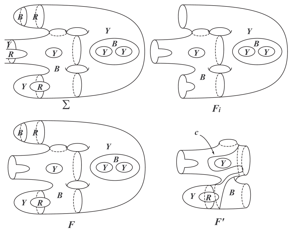
Let be the union of the components of that are disks (possibly, ). Let . By construction, every component of is essential in (possibly, ). Thus, a closed curve of is essential in if and only if it is essential in . Since , if then ; if, on the other hand, , then and in particular, ; we conclude that in either case . Thus some component of cut open along , denoted by , has . Note that every curve of is essential in . By construction, . Let be the union of the disks bounded by outermost curves of and the disks . Note that consists of disks, and is entirely blue or yellow; in Figure 1, consists of two disks, one of each kind.
Assume first that . Let be a curve, parallel to a component of , that decomposes as , where is an annulus. By isotopy of in we may assume that . We see that is entirely blue or yellow, , and is essential in .
Next assume that (that is, ). Let be a separating, essential curve in . By isotopy of we may assume that is contained in one component of cut open along . Let be the other component. We conclude that in this case too, is entirely blue or yellow, , and is essential in .
Let , , and be three curves that are essential in (and hence in ) and co-bound a pair of pants, denoted by , in . It is easy to see that , , , and have the properties listed in Proposition 5.6. ∎
Since it is on the boundary of the total space of an -bundle in (). The other component of the associated -bundle is a pair of pants denoted by . The components of are denoted by , , and so that is parallel to , is parallel to , and is parallel to . Since , every point of is yellow or red; we conclude that . Hence the -bundle in is trivial. The annulus extended from to (resp. to , to ) in is denoted by (resp. , ). By construction, these annuli are embedded. Note that is possible.
Lemma 5.7.
One of the following holds:
-
(1)
After renaming if necessary, and are not boundary parallel, and , , and are boundary parallel.
-
(2)
.
Proof.
We claim that one of , or is not boundary parallel in (). Suppose, for a contradiction, that , , are all boundary parallel. Let be the annulus that is parallel to. Since is an essential pair of pants it is not contained in ; it is easy to see that the intersection of the region of parallelism between and and the trivial -bundle in is exactly ; similarly we treat and . We see that is homeomorphic to the trivial -bundle, and hence is a genus 2 handlebody. This contradicts our assumption that .
Therefore one of , or is not boundary parallel, and after renaming if necessary we may assume it is . We may assume is boundary parallel, for otherwise by Lemma 4.4 (1). Similarly, one of , or is not boundary parallel, after renaming if necessary we may assume it is , while is boundary parallel. Finally by Lemma 4.4 (1) we may assume that or is boundary parallel, say . ∎
Lemma 5.8.
One of the following holds:
-
(1)
, and are essential in , and is not isotopic in to , or .
-
(2)
.
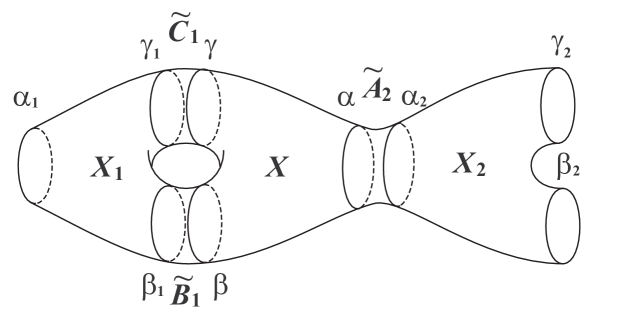
Proof.
We may assume that Conclusion (1) of Lemma 5.7 holds; thus , and are boundary parallel. We denote by the annuli to which , , and are parallel (respectively). See Figure 2, where , but this need not be the case.
If is inessential in , then we may cap off, and after a small isotopy we obtain a meridian disk with . Using and , Lemma 4.4 (2) shows that . Similarly if (resp. ) is inessential in then (resp. ) bounds a meridian disk . Using and , Lemma 4.4 (2) shows that .
If is isotopic to in then either the annulus connecting the two contains or . The former is impossible since is an essential pair of pants and the latter contradicts the assumption .
Let be a closed curve constructed by pasting together four arcs, the first connecting to in , the second connecting to in , the third connecting to in , and the final arc connecting to in . Since , we have . By construction . Therefore is not isotopic in to either or . ∎
6. Proof of Theorem 1.8
With notation as in Section 5 we assume, as we may by Lemma 5.7, that and are not boundary parallel and that , , and are boundary parallel. We assume, as we may by Lemma 5.8, that , and are essential in and is not isotopic in to , or .
The proof is divided into the following two cases:
Case One. can be isotoped to be disjoint from . Let , , and be as in Lemma 5.8. Let be the twice punctured torus . Isotope so that . After this isotopy, . Hence either or . In the former case, . Since is isotopic to in , is isotopic into . By Proposition 5.6(2) is essential, and hence is isotopic to a component of , contradicting our assumptions.
Hence we may assume that . Let be a meridian disk obtained by compressing or boundary compressing . After a small isotopy we may assume that , and hence either (hence ) or (hence ). Thus is disjoint from at least one component of ; by Lemma 4.4 (2), , proving Theorem 1.8 in Case One.
Before proceeding to Case Two we refine our colorings. Let be an -equivalent family of faces, ordered as so that is -adjacent to (). Then the red faces are , , , and . We color and dark red. If we color and light red.
Clearly, a face is -adjacent to two distinct faces if and only if it is colored blue, yellow, or light red. Let be a point on such a face. Then is on the boundary of two -fibers, on the and sides. Denote the other endpoints of these fibers by and . By construction we see that the colors at , and fulfill the conditions in Table 1.
| , | |
|---|---|
| blue | yellow or light red |
| yellow | blue or light red |
| light red | one is dark red and the other can be any color |
Notation 6.1.
Every light red face is -equivalent to a dark red face on one side. On the other side it is -equivalent to a face that may be blue, yellow, light red or dark red. This decomposes the set of light red points into four disjoint subsets. We label a light red face that is -equivalent to a blue (resp. yellow) face by lr[b] (resp. lr[y]).
Case Two. cannot be isotoped to be disjoint from . Since , each point of is yellow or light red. Hence bounds -bundles on both sides. Let be the be the (possibly immersed) -bundle obtained by extending into , and denote by ; see Figure 3.
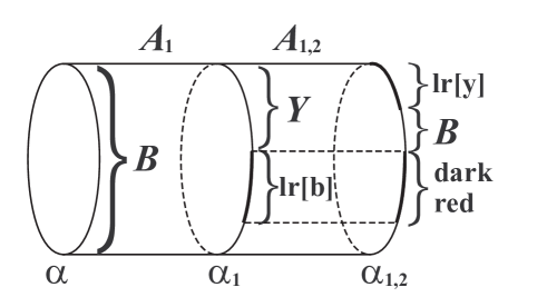
Since every point of is yellow or light red and labeled lr[b], every point of is blue, light red and labeled lr[y], or dark red (see Table 1 and Notation 6.1). Thus , and we see that is trivial -bundle, that is, an embedded annulus.
Since and co-bound an -bundle, every point of is yellow or light red and labeled lr[b]. Thus . By assumption cannot be isotoped off . Hence is not isotopic to ; this implies that is not boundary parallel. By assumption is not boundary parallel and is essential in . Applying Lemma 4.4 (1) to , , and we conclude that , completing the proof of Theorem 1.8.