HyperLoRA for PDEs

We consider Partial Differential Equations of the form

$$N[x,t,u(x,t)]=0,t\in[0,T],x\in\Omega$$

(1)

Here, $N$ is a non-linear differential operator consisting of space and time derivatives of spatial variable $x$ and temporal variable $t$. The neural network is trained using a loss function that consists of: 1) A supervised initial condition loss $L_{IC}$ and boundary condition loss $L_{BC}$ component and 2) An unsupervised physics-informed loss component.

	$\displaystyle L(\theta)$	$\displaystyle=L_{IC}(\theta)+L_{BC}(\theta)+L_{Physics}(\theta)$
	$\displaystyle L_{IC}(\theta)$	$\displaystyle=\sum_{x_{i}\in IC}(u(x_{i},0)-f(x_{i}))^{2}$
	$\displaystyle L_{BC}(\theta)$	$\displaystyle=\sum_{x_{bc},t_{bc}\in BC}(u(x_{bc},t_{bc})-h(x_{bc},t_{bc}))^{2}$
	$\displaystyle L_{Physics}(\theta)$	$\displaystyle=\sum_{x,t\in C}N(u,x,t,u_{t},u_{x},u_{xx},\text{...})^{2}$		(2)

Here, C represents the set of collocation points on which the Physics-loss is calculated. IC, BC represents the set of points at which Initial Conditions and Boundary Conditions are evaluated. $f$,$h$, represent the initial condition and boundary condition functions respectively. $\theta$ represents the weights of the neural network.

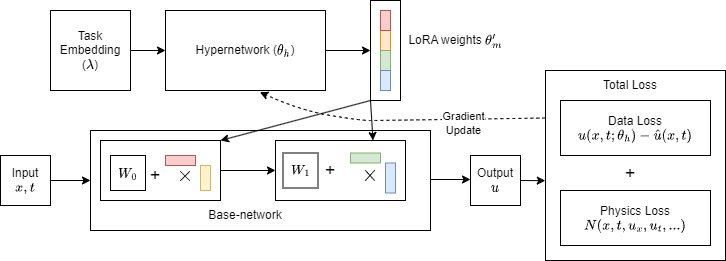
We follow the methodology as proposed in (Hu et al. 2021). We first train a PINN on task $T_{0}$ and represent it’s weights as $W_{0}$. Now, we represent the weights of a task $T_{1}$ as $W_{1}$ and represent it’s update as follows:

$$W_{1}=W_{0}+\Delta W=W_{0}+A\cdot B\\$$

(3)

Here, $W_{1}\in R^{m\times n}$,$W_{0}\in R^{m\times n}$, $B\in R^{m\times r}$, $A\in R^{r\times n}$. Here $r<$min{$m,n$}. During train time, $W_{0}$ is kept frozen and matrices $A,B$ contain trainable parameters which adapt from task $T_{0}$ to task $T_{1}$.

Hypernetworks (Ha, Dai, and Le 2016) are neural networks parameterized by $\theta_{h}$ which accept a task-representation $\lambda$ as input and predict weights $\theta_{m}$ of a neural network $M$ used to model that particular task.

	$\displaystyle\theta_{m}$	$\displaystyle=H(\lambda;\theta_{h})$
	$\displaystyle\textbf{u}(x,t)$	$\displaystyle=M(x,t;\theta_{m})$		(4)

Here $\theta_{m}$ is directly supplied to the main-network for evaluating the solution $\textbf{u}_{pinn}$. We sample different values of $\lambda$ to train the hypernetwork, and generalize to unseen $\lambda$ values at test-time.

LoRA-based Hypernetworks are a combination of Hypernetworks and low-ranked adaptation of the main-network. The mathematical formulation is defined as follows:

	$\displaystyle\theta^{\prime}_{m}$	$\displaystyle=H(\lambda;\theta_{h})$
	$\displaystyle\theta_{m}$	$\displaystyle=W_{0}+\theta^{\prime}_{m}$
	$\displaystyle\textbf{u}(x,t)$	$\displaystyle=M(x,t;\theta_{m})$		(5)

Here, $W_{0}$ refers to the weights of a pretrained main-network for a task $T_{0}$. The Hypernetwork $H$, instead of predicting the weights of the entire main-network $M$, just predicts the low ranked weights $A,B$ represented by $\theta^{\prime}_{m}=[A:B]$.

HyperPINNs are hypernetworks trained using physics-informed loss introduced in (de Avila Belbute-Peres, fan Chen, and Sha 2021) to solve parameterized differential equations.

	$\displaystyle\theta_{m}$	$\displaystyle=H_{pinn}(\lambda;\theta_{h})$
	$\displaystyle\textbf{u}_{pinn}(x,t)$	$\displaystyle=M_{pinn}(x,t;\theta_{m})$		(6)

HyperPINN consists of two components, a hypernetwork $H_{pinn}$ and a main-network $M_{pinn}$. $H_{pinn}$ takes in task parameterization $\lambda_{h}$ as input and outputs the weights of the main-network $\theta_{m}$.

We combine LoRA-based adaptation and HyperPINNs to solve for parameterized PDEs while having to predict a lower number of parameters against a standard HyperPINN. The mathematical formulation of LoRA-based HyperPINN is defined as follows:

	$\displaystyle\theta^{\prime}_{m}$	$\displaystyle=H_{pinn}(\lambda;\theta_{h})$
	$\displaystyle\theta_{m}$	$\displaystyle=W_{0}+\theta^{\prime}_{m}$
	$\displaystyle\textbf{u}(x,t)$	$\displaystyle=M_{pinn}(x,t;\theta_{m})$		(7)

We provide an illustration of LoRA-based HyperPINN in figure 1.

Instead of using supervised data or physics-informed loss to train the Hypernetwork, Majumdar et al. directly perform regression in weight-space on pretrained PINN weights.

	$\displaystyle\theta_{m}$	$\displaystyle=H(\lambda;\theta_{h})$
	$\displaystyle\textbf{u}(x,t)$	$\displaystyle=M(x,t;\theta_{m})$		(8)

Here, the hypernetwork $H$ is trained using $\mathbb{E}_{t\sim T}[(\theta_{m}-\theta_{t})]^{2}$, where $T$ refers to the task space and $\theta_{t}$ refers to weights of pretrained PINN for task $t$.

Instead of predicting weights of the entire network, Hypernetwork $H$ just predicts the LoRA decomposed weights. Remaining methodology follows from the previous subsection.

The governing PDE system of one-dimensional Burger’s equation is given by:

	$\displaystyle u_{t}+u^{2}_{x}(x,t)/2$	$\displaystyle=\nu u_{xx}$
	$\displaystyle u(x,0)$	$\displaystyle=u_{0}(x)$		(9)

Here, $\Omega\in[0,1]$,$\nu=0.01$ refers to the viscosity of the system, and $u_{0}\in L^{2}_{per}((0,1);R)$ refers to the initial condition sampled from $\mu$ where $\mu=N(0,625(-\Delta+25I)^{-2})$.

The governing equations of two-dimensional coupled viscous Burger’s equation is given by:

	$\displaystyle u_{t}+u*u_{x}+v*u_{y}$	$\displaystyle=\nu*(u_{xx}+u_{yy})$
	$\displaystyle v_{t}+u*v_{x}+v*v_{y}$	$\displaystyle=\nu*(v_{xx}+v_{yy})$		(10)

The initial and boundary conditions are sampled from the true analytical solutions of the PDE, given by:

	$\displaystyle u(x,y,t)$	$\displaystyle=\frac{3}{4}+\frac{1}{4(1+exp(\frac{(-4x+4y-t)}{32\nu}))}$
	$\displaystyle v(x,y,t)$	$\displaystyle=\frac{3}{4}-\frac{1}{4(1+exp(\frac{(-4x+4y-t)}{32\nu}))}$		(11)

Here $\Omega\in[0,1]^{2}$, $t\in[0,1]$, $\nu$ refers to the viscosity of the flow. We consider $\nu\in[1e^{-4},1e^{-3}]$ for our experiments.

Navier-Stokes: Kovasznay flow is a two-dimensional steady state laminar flow. The governing Partial Differential equations are given by:

	$\displaystyle u_{x}+v_{y}$	$\displaystyle=0$
	$\displaystyle u*u_{x}+v*u_{y}$	$\displaystyle=-p_{x}+(u_{xx}+u_{yy})/Re$
	$\displaystyle u*v_{x}+v*v_{y}$	$\displaystyle=-p_{y}+(v_{xx}+v_{yy})/Re$		(12)

The boundary conditions for the equation are sampled from the true analytical solutions of the PDE, given by:

	$\displaystyle u_{true}$	$\displaystyle=1-e^{\lambda x}cos(2\pi y)$
	$\displaystyle v_{true}$	$\displaystyle=\lambda e^{\lambda x}sin(2\pi y)/2\pi$
	$\displaystyle p_{true}$	$\displaystyle=(1-e^{2\lambda x})/2$		(13)

Here, $\Omega\in[0,1]^{2}$, $\lambda=\frac{Re}{2}-\sqrt{\frac{Re^{2}}{4}+4\pi^{2}}$, where $Re$ refers to the Reynold’s number of the system. We consider $Re\in[20,100]$ for our experiments.

In this subsection, we analyze how the performance varies by changing the rank of our decomposed matrices of Neural network used for low-ranked adaptation. We tabulate the results of our Low-ranked adaptation experiments in Table 1. Our experimental design is as follows: Across all PDE examples, we first train an independent PINN on a task $T_{0}$. Then we perform Low-ranked adaptation for a new task $T_{x}$ using the trained PINN for task $T_{0}$ as our base model. Lower the rank of the decomposed tensors, the fewer the number of parameters involved in adapting to the newer task.

Across all three PDE systems, we notice the average accuracy across the test-tasks first increases with increase in rank, reaches an optimal rank, which happens to be 4, and then slightly deteriorates as the rank is further increased to the full rank of the original matrix. The best LoRA-based PINN is on average 3.98$\times$ better than PINNs, while requiring $8.22\times$ fewer parameters, $2.5\times$ fewer epochs while yielding $5.25\times$ faster training time per epoch (due to training fewer parameters). Additionally, the best LoRA-based PINN is on average $2.23\times$ better than a finetuned-PINN, while requiring $8.22\times$ fewer parameters, $2\times$ fewer epochs yielding $5.25\times$ faster training time per epoch.

Improvement of performance due to initial rank increase can be attributed to improved representation capacity of the finetuned task $T_{x}$ due to higher number of parameters. We see a 2.78% improvement in 1D-Burger’s, 2.11% improvement in Navier-Stokes, and 32.56% improvement in 2D-Burger’s on increasing the rank from 1 to 4. We additionally notice, while the training-time per epoch is lower for LoRA-based PINNs with ranks 1 and 2, as the representation capacity is restricted, these take a higher time to converge as compared to LoRA-based PINNs with rank 4. Further increase in rank leads to drop in performance, and we speculate overfitting and increased in variance to be reasons for it due to increase in # parameters. In addition, very high ranked LoRA-based PINNs require higher training time to converge, as against the best-ranked LoRA-based PINN.

In this subsection, we study the results for our experiments for LoRA-based HyperPINNs. Hypernetwork-based PINN architectures have faster inference time than PINN-based counterparts, and allows for generalization to parameterized PDE systems. We tabulate the results in Table 2. Across all examples, * refers to the case where we don’t perform LoRA, and hypernetwork predicts the entire neural network.

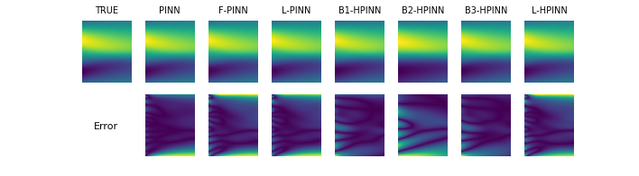
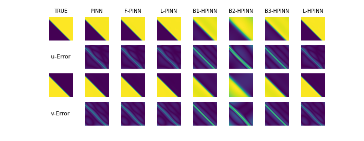
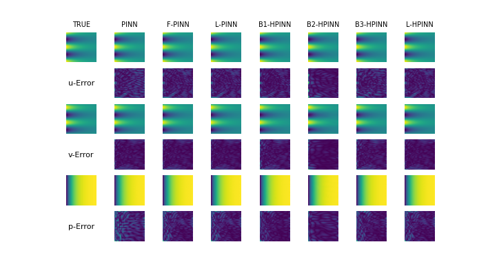
As our first benchmark, we train a LoRA-based hypernetwork using the true simulation data and solutions of the PDE as ground-truth. Similar to our analysis in previous subsection, we observe, across all PDE examples, the Hypernetwork performance improves till LoRA of rank 4, and then starts deteriorating. The reason for improved performance for rank 4 over lower ranks is higher representation capacity of base-networks. The reason for drop in performance for Hypernetworks beyond rank 4 is inability of Hypernetworks to predict very high dimensional weights in a regression setting. However, on test tasks, Rank-4 LoRA-based hypernetworks are just $1.35\times$ worse than Rank-4 LoRA-based PINNs on Kovasznay flow, but are $10.15\times$ and $460\times$ worse on 2D-Burger’s and 1D-Burger’s respectively. Thus, this benchmark has two issues. First, this benchmark requires pre-existing simulation data for multiple solved PDE instances which may not be available in practice, and second, the generalization is poor and physics is violated as seen in Figures 2, 3, 4.

We mitigate the data availability drawback by training multiple instances of PINNs and use the weights of the data generated by trained-PINNs as supervised labels for benchmark 2. In our second benchmark, we use the hypernetwork to predict the weights of the base-network and use weights of the pre-trained PINNs as regression loss following motivations from the paper (Majumdar et al. 2022). While the rank analysis remains similar and the hypernetwork has lower training time, the performace across all test-examples is quite poor. Reason: Weight-spaces are extremely sensitive to slight perturbations, thus leading to very complex manifolds being learnt. The complexity of generalizing the output manifold to test-examples is increased, thus leading to poor performance. Weight-regressor hypernetworks typically perform 2-3 orders worse than LoRA-based PINNs and benchmark 1.

In benchmark 3, we use the data generated by trained-PINNs as supervised labels and train a hypernetwork. We observe, the rank analysis to be similar as in the past sections, and the best-ranked hypernetwork performs comparably ($1.02\times$ worse) to the best-ranked hypernetwork in benchmark 1, and is 3-4 orders superior in performance as compared to weight-regressor hypernetworks. However, this benchmark like benchmark 1 performs similarly worse ($1.36\times$,$4.19\times$ and $463\times$) than LoRA-based PINNs of rank 4 on Kovasznay flow, 2D Burger’s and 1D Burger’s respectively. As a summary, this benchmark has 2 issues: 1) Training multiple PINNs can be costly 2) Poor generalization and violation of physics constraints, as seen in Figure 2, 3, 4.

We mitigate both the issues in benchmark 3 by using LoRA-based HyperPINNs. HyperPINNs take in a task embedding as input, and learn the hypernetworks in a physics-informed manner, instead of taking pre-trained data as a supervision signal. This eradicates the need of having ground-truth samples or neural surrogate samples like in benchmark 3. We observe the performance of Rank 4 LoRA-based HyperPINN is 3 and 2 orders of magnitude better in 1D-Burger’s equation and 2D-Burger’s equation respectively, and is less-than an order ($3.61\times$) worse than LoRA-based PINNs on test-examples. This indicates LoRA-based HyperPINNs have the capability to generalize across test-tasks at an inference-time advantage, compared to traditional PINNs and LoRA-based PINNs, while respecting the physics constraints observed in Figures 2, 3, 4.

We tabulate the inference time for our architectures in Table 3. Across all examples, we observe LoRA-based HyperPINNs to be around 2-3 orders of magnitude faster than vanilla architectures, as the entire computational cost is transferred to one-time train cost, and we simply predict the weights for a test-time, without having to finetune. The best-ranked LoRA-based PINNs are $10.25\times$ faster than finetuned PINNs and $13.21\times$ faster than vanilla-PINNs, due to training lower number of parameters and incorporating pre-trained information from an already trained base-task.

References

- de Avila Belbute-Peres, fan Chen, and Sha (2021) de Avila Belbute-Peres, F.; fan Chen, Y.; and Sha, F. 2021. HyperPINN: Learning parameterized differential equations with physics-informed hypernetworks. arXiv:2111.01008.
- Dupont et al. (2022) Dupont, E.; Kim, H.; Eslami, S. M. A.; Rezende, D.; and Rosenbaum, D. 2022. From data to functa: Your data point is a function and you can treat it like one. arXiv:2201.12204.
- Greenfeld et al. (2019) Greenfeld, D.; Galun, M.; Basri, R.; Yavneh, I.; and Kimmel, R. 2019. Learning to optimize multigrid PDE solvers. In International Conference on Machine Learning, 2415–2423. PMLR.
- Guo, Li, and Iorio (2016) Guo, X.; Li, W.; and Iorio, F. 2016. Convolutional Neural Networks for Steady Flow Approximation. In Proceedings of the 22nd ACM SIGKDD International Conference on Knowledge Discovery and Data Mining, KDD ’16, 481–490. New York, NY, USA: Association for Computing Machinery. ISBN 9781450342322.
- Ha (2016) Ha, D. 2016. Generating Large Images from Latent Vectors. blog.otoro.net.
- Ha, Dai, and Le (2016) Ha, D.; Dai, A.; and Le, Q. V. 2016. HyperNetworks. arXiv:1609.09106.
- Hu et al. (2021) Hu, E. J.; Shen, Y.; Wallis, P.; Allen-Zhu, Z.; Li, Y.; Wang, S.; Wang, L.; and Chen, W. 2021. LoRA: Low-Rank Adaptation of Large Language Models. arXiv:2106.09685.
- Ivison et al. (2023) Ivison, H.; Bhagia, A.; Wang, Y.; Hajishirzi, H.; and Peters, M. 2023. HINT: Hypernetwork Instruction Tuning for Efficient Zero- Few-Shot Generalisation. arXiv:2212.10315.
- Kochkov et al. (2021) Kochkov, D.; Smith, J. A.; Alieva, A.; Wang, Q.; Brenner, M. P.; and Hoyer, S. 2021. Machine learning–accelerated computational fluid dynamics. Proceedings of the National Academy of Sciences, 118(21): e2101784118.
- Li and Liang (2021) Li, X. L.; and Liang, P. 2021. Prefix-Tuning: Optimizing Continuous Prompts for Generation. arXiv:2101.00190.
- Li et al. (2020) Li, Z.; Kovachki, N.; Azizzadenesheli, K.; Liu, B.; Bhattacharya, K.; Stuart, A.; and Anandkumar, A. 2020. Fourier neural operator for parametric partial differential equations. arXiv preprint arXiv:2010.08895.
- Lu, Jin, and Karniadakis (2019) Lu, L.; Jin, P.; and Karniadakis, G. E. 2019. Deeponet: Learning nonlinear operators for identifying differential equations based on the universal approximation theorem of operators. arXiv preprint arXiv:1910.03193.
- Majumdar et al. (2022) Majumdar, R.; Jadhav, V.; Deodhar, A.; Karande, S.; Vig, L.; and Runkana, V. 2022. Real-time Health Monitoring of Heat Exchangers using Hypernetworks and PINNs. arXiv:2212.10032.
- Mescheder et al. (2019) Mescheder, L.; Oechsle, M.; Niemeyer, M.; Nowozin, S.; and Geiger, A. 2019. Occupancy Networks: Learning 3D Reconstruction in Function Space. In Proceedings of the IEEE/CVF Conference on Computer Vision and Pattern Recognition (CVPR).
- Raissi, Perdikaris, and Karniadakis (2019) Raissi, M.; Perdikaris, P.; and Karniadakis, G. 2019. Physics-informed neural networks: A deep learning framework for solving forward and inverse problems involving nonlinear partial differential equations. Journal of Computational Physics, 378: 686–707.
- Ruiz et al. (2023) Ruiz, N.; Li, Y.; Jampani, V.; Wei, W.; Hou, T.; Pritch, Y.; Wadhwa, N.; Rubinstein, M.; and Aberman, K. 2023. HyperDreamBooth: HyperNetworks for Fast Personalization of Text-to-Image Models. arXiv preprint arXiv:2307.06949.