Hyperons during proto-neutron star deleptonization and the emission of dark flavoured particles
Abstract
Complementary to high-energy experimental efforts, indirect astrophysical searches of particles beyond the standard model have long been pursued. The present article follows the latter approach and considers, for the first time, the self-consistent treatment of the energy losses from dark flavoured particles produced in the decay of hyperons during a core-collapse supernova (CCSN). To this end, general relativistic supernova simulations in spherical symmetry are performed, featuring six-species Boltzmann neutrino transport, and covering the long-term evolution of the nascent remnant proto-neutron star (PNS) deleptonization for several tens of seconds. A well-calibrated hyperon equation of state (EOS) is therefore implemented into the supernova simulations and tested against the corresponding nucleonic model. It is found that supernova observables, such as the neutrino signal, are robustly insensitive to the appearance of hyperons for the simulation times considered in the present study. The presence of hyperons enables an additional channel for the appearance of dark sector particles, which is considered at the level of the hyperon decay. Assuming massless particles that escape the PNS after being produced, these channels expedite the deleptonizing PNS and the cooling behaviour. This, in turn, shortens the neutrino emission timescale. The present study confirms the previously estimated upper limits on the corresponding branching ratios for low and high mass PNS, by effectively reducing the neutrino emission timescale by a factor of two. This is consistent with the classical argument deduced from the neutrino detection associated with SN1987A.
1 Introduction
Massive stars end their lifes in the event of a CCSN, when the stellar core collapses due to pressure losses from electron captures on protons bound in iron-group nuclei and the photodissociation of nuclei. The core collapse halts when the density exceeds the normal nuclear density, and the stellar core bounces back with the formation of a shock wave. The initial propagation of this bounce shock leads to the release of a -burst when reaching the neutrinospheres of the last inelastic scattering. The associated energy loss, in combination with the energy loss due to the photodissociation of the still infalling matter onto the expanding dynamic bounce shock, causes the latter to stall and turn into an accretion shock. Revival of this standing accretion shock is considered the CCSN explosion engine (for recent reviews, c.f., Refs. [1, 2, 3] and references therein).
Most of the gravitational binding energy gain is stored in the central compact PNS, in the magnetic-rotational energy [4], as well as in thermal degrees of freedom and neutrinos of all flavours, on the order of several erg. Hence, the neutrino-heating mechanism for shock revival, first proposed in ref. [5], has long been studied in modern CCSN simulations. These are based in multi-dimensional neutrino radiation hydrodynamics featuring neutrino transport, where in the presence of multi-dimensional hydrodynamics phenomena, such as convection and hydrodynamic instabilities, the neutrino-heating efficiency increases, compared to spherically symmetric CCSN models, which therefore generally fail to yield CCSN explosions. There are two exceptions, (i) low-mass stellar progenitors in the zero-age main sequence (ZAMS) mass range of 8–10 M⊙ [6, 7, 8] as well as ultra-stripped stellar progenitors that result from binary evolution [9, 10], despite substantial differences between spherically symmetric and multi-dimensional simulations [11, 12, 13, 14, 15], and (ii) CCSN explosions triggered due to a sufficiently strong first-order phase transition from normal nuclear matter to the quark-gluon plasma at high baryon density (c.f. Refs. [16, 17, 18, 19, 20, 21] and references therein) as well as the spontaneous scalarization of beyond the standard model degrees of freedom [22].
The latter CCSN explosion mechanism relates to one of the largest uncertainties in CCSN modelling, namely, the state of matter under CCSN conditions, i.e. at high baryon density, in excess of saturation density, large isospin asymmetry given by the hadronic charge density (the proton abundance in the absence of other charged hadronic resonances, on the order of –) and temperatures on the order of several tens of MeV (for a recent review of the role of the EOS in simulations of CCSN, see ref. [23]). Besides the QCD deconfinement phase transition, which has lately been explored extensively also in the context of binary neutron star mergers [24, 25], the impact of hadronic degrees of freedom has been studied in the context of failed CCSN in Refs. [26, 27, 28, 29, 30], even though the potential impact of strange, as well as non-strange hadronic degrees of freedom has long been studied for neutron stars (see recent reviews [31, 32, 33, 34] and references therein.) Thereby, particular emphasis has been placed on the hyperon puzzle, which is related to the softening of the supersaturation density EOS due to the presence of additional, heavy hadronic degrees of freedom, potentially violating the maximum neutron star mass constraint of about M⊙, the latter was derived from observations of massive pulsars [35, 36, 37, 38, 37, 39]. Several possible solutions have been widely discussed in the literature. Among them, it has been put forward an early onset of the quark-hadron deconfinement phase transition at densities below which strange hadronic resonances would appear, or the existence of much more repulsive hadronic interactions at high baryon densities. However, hyperon-nucleon and hyperon-hyperon interactions are less understood than nucleon-nucleon interactions, due to the sparse knowledge of scattering data. This makes their potentials poorly constrained and dynamics far from understood (c.f. ref. [40] and references therein). The theoretical understanding has been brought forward to solve the problem of thermal production of hyperons at low baryon density for heavy-ion physics based on the coupled channel approach (c.f. Refs. [41, 42, 43] and references therein) and furthermore, final-state interaction analyses [44, 45, 46, 47] as well as femtoscopy studies (see ref. [48] for a review and references therein) have become available as well as data on hypernuclear structure [49, 50, 51].
Due to the poorly known hyperon EOS at high baryon density, effective hyperonic model EOS have long been employed in astrophysical studies, e.g., based on the relativistic mean-field (RMF) approach that treats the unknown interactions via baryon-meson couplings. The present article implements the FSU2H∗ hyperonic relativistic mean field model in simulations of CCSN, focusing on the PNS deleptonization phase, i.e. the evolution after the CCSN explosion onset has been triggered during which the nascent PNS deleptonizes via the emission of neutrinos of all flavours on a timescale of 10 seconds. This phase is ideal for studying the impact of hadronic physics as the central density increases continuously as a direct consequence of the deleptonization.
The requirements for multi-purpose EOS for applications of CCSN studies is to cover a large parameter space. Therefore, the RMF framework has long been developed (for recent reviews, see Refs. [52, 53] and references therein). Recent reviews of the RMF framework for hyperon EOS can be fond in ref. [54, 33]111Note the existence of the online service CompOSE repository that provides data tables for different state of the art EOS ready for use in astrophysical applications, nuclear physics and beyond [55, 56]..
In addition to the impact that hyperons can potentially have in CCSN through the EOS, they can open potentially new cooling channels with the emission of novel, yet hypothetical, particles from the interior of the PNS. In particular, if the net energy carried away by these particles is comparable to that of neutrinos, then significant changes in the neutrino signal are predicted. These can be tested using the neutrino flux that was observed from SN1987A [57, 58]. Such phenomenology has been studied extensively in the context of the QCD axions, produced in the stellar plasma by, e.g. nucleon-nucleon bremsstrahlung [59, 60, 61, 62, 63, 64, 65], from pions studied [66] and in simulations [67], and has been extended to many other “dark-sector” theories predicting the existence of new weakly interacting particles with mass [68, 69, 70, 71, 72, 73], which is on the order of few tens of MeV.
Adding “standard” degrees of freedom in the plasma, on top of nucleons and electrons/positrons, can also extend these analyses, as was recently demonstrated in the case of muons (c.f. Refs. [74, 75, 76, 77, 73] and references therein), for pions [78, 79, 80, 66, 67, 81], and for hyperons [82, 83, 84, 85]. In the case of hyperons, this was studied for various models that can induce flavour-changing neutral currents, such as the following decays, and , where the energy difference between final and initial states is considered to be carried away by dark degrees of freedom. Therefore, results of spherically symmetric simulations were employed without exotic cooling and implementing conventional EOS without hyperons. To establish limits on these models, the impact of the new dark emission on the dynamics of the CCSN was neglected, and thermodynamic quantities such as chemical potentials were re-derived by using interpolation tables of the hyperonic extensions of the EOS used in the simulations (see also ref. [85] for a slightly different approach).
A dark sector coupled to quarks can have a rich flavour structure that is subject to strangeness-changing neutral currents (for reviews, see Refs. [86, 87]). One prototypical example of these dark flavoured sectors is the QCD axion, with non-diagonal flavour couplings, known as “familon”. This was first predicted in refs. [88, 89] as a consequence of jointly solving the strong CP and flavour problems, and was further developed [90, 91, 92, 82, 93]. Other examples include the dark photon, which interacts with standard-model fermions only through non-renormalizable operators (see Refs. [94, 95, 96, 97] and references therein) or dark baryons [84]. The latter are neutral fermions with masses of 1 GeV endowed with baryon number and that can be part of dark matter, and explain baryogenesis (c.f. Refs. [98, 99]) and the neutron lifetime puzzle [100]. The self-consistent implementation of hyperons in CCSN simulations enables us to overcome previous limitations (c.f. ref. [83] and references therein), studying the feedback of dark boson production on the supernova dynamics and neutrino emission.
The paper is organized as follows. In section 2 the RMF framework for reference nucleonic and hyperonic EOS will be introduced, which is evaluated at selected conditions in section 3, including finite temperature, and discussed accordingly. CCSN simulations will be launched and evaluated in section 4. The comprehensive analysis from the impact of dark bosons will be provided in section 5 and the manuscript closes with a summary in section 6.
2 Hyperons within the relativistic mean field framework
The present study of the impact of strange degrees of freedom in CCSN simulations employed the FSU2H∗ RMF EOS. In this framework, the interactions between the baryons are mediated via the exchange of virtual mesons, based on the following Lagrangian for baryons and mesons ,
| (2.1) |
with
| (2.2) | |||||
and
| (2.3) | |||||
The quantity represents the baryon Dirac field and indicates the mass of particle , while the mesons that mediate the interaction between the baryons are two isoscalar-scalar mesons ( and ), two isoscalar-vector mesons ( and ), and one isovector-vector meson (). The mesonic strength tensors are labeled with , , and , whereas are the Dirac matrices, labels the coupling of baryon to meson and is the isospin operator. We stress that, since we are dealing with charge-neutral objects in the absence of magnetic fields, the electromagnetic part of the Lagrangian does not play a role.
| MeV | MeV | MeV | MeV | MeV | ||||||||||
| 497.479 | 782.5 | 763 | 980 | 1020 | 102.72 | 169.53 | 197.27 |
| MeV | |||||||||
| 4.0014 | -0.0133 | 0.008 | 0.045 |
In order to determine the EOS of the system, one first needs to obtain the Euler-Lagrange equations of motion for each particle. Then, a closed set of equations can be obtained by using the mean-field approximation that allows for the meson fields to be replaced by their expectation values, as well as by coupling those equations with the weak interaction equilibrium condition and baryon and charge conservation number equations. The solution of this set fixes the composition of matter and the values of the meson fields. Finally, from the stress-energy tensor all thermodynamic quantities can be obtained, such as the pressure and energy density (for details on the set of equations to be solved, we refer the reader to the Refs. [101, 102, 103, 104] and references therein).
We show in the following the explicit form of the effective mass and chemical potential of the different species, since these are important quantities whose behaviour influences the thermal evolution in CCSN explosions. The effective mass of a given particle reads as follows,
| (2.4) |
where the expectation values of the scalar mesons, denoted as and , govern their behaviour. Since no isospin splitting is considered due to the absence of the meson channel, MeV is used in FSU2H∗ for the nucleon rest masses while those of the hyperons are given in the Particle Data Booklet [105]. The expectation values of the vector mesons, i.e. , and , control the different chemical potentials as follows,
| (2.5) |
with the thermodynamic chemical potential . We note that the hidden mesons and are coupled only to particles with non-zero strangeness.
3 Equation of state with hyperons
The different parameters of the FSU2H∗ model are chosen so as to predict an EOS that is compatible with the constraints coming from heavy ion collisions as well as those obtained from the saturation properties of nuclear matter and finite nuclei. At the same time the model predicts a maximum neutron star mass that is above 2.0 M⊙ and a radius about 13 km for canonical neutron stars of 1.4 M⊙ (for details, see Refs. [101, 102]). This model was then extended to finite temperature [103], whereas more recently the hyperonic uncertainties have been analyzed for the determination of the masses, radii, tidal deformabilities and moments of inertia, both at zero and finite temperatures [104]. Indeed, the FSU2H∗ model is compatible with the tidal deformability extracted from the GW170817 event [106] as well as the NICER determinations on radii [107, 108, 109, 110]. The values of the parameter meson masses and meson-nucleon coupling constants can be found in Table 1, whereas the other parameters of the Lagrangian (2.3) are given in Table 2. The ratios of coupling constants of hyperons to mesons are give in Table 3.
In the present work we make use of the FSU2H∗ model in two different ways. Firstly, a set of simulations is performed with the exact FSU2H∗ EOS, and the results of those simulations are referred as HYPERONS. The results of the second set of simulations, that will be referred as NUCLEONS, are obtained within the same FSU2H∗ model, but preventing the appearance of hyperons by setting their masses to infinity. This set is necessary in order to quantify the impact that hyperons have on the observables.
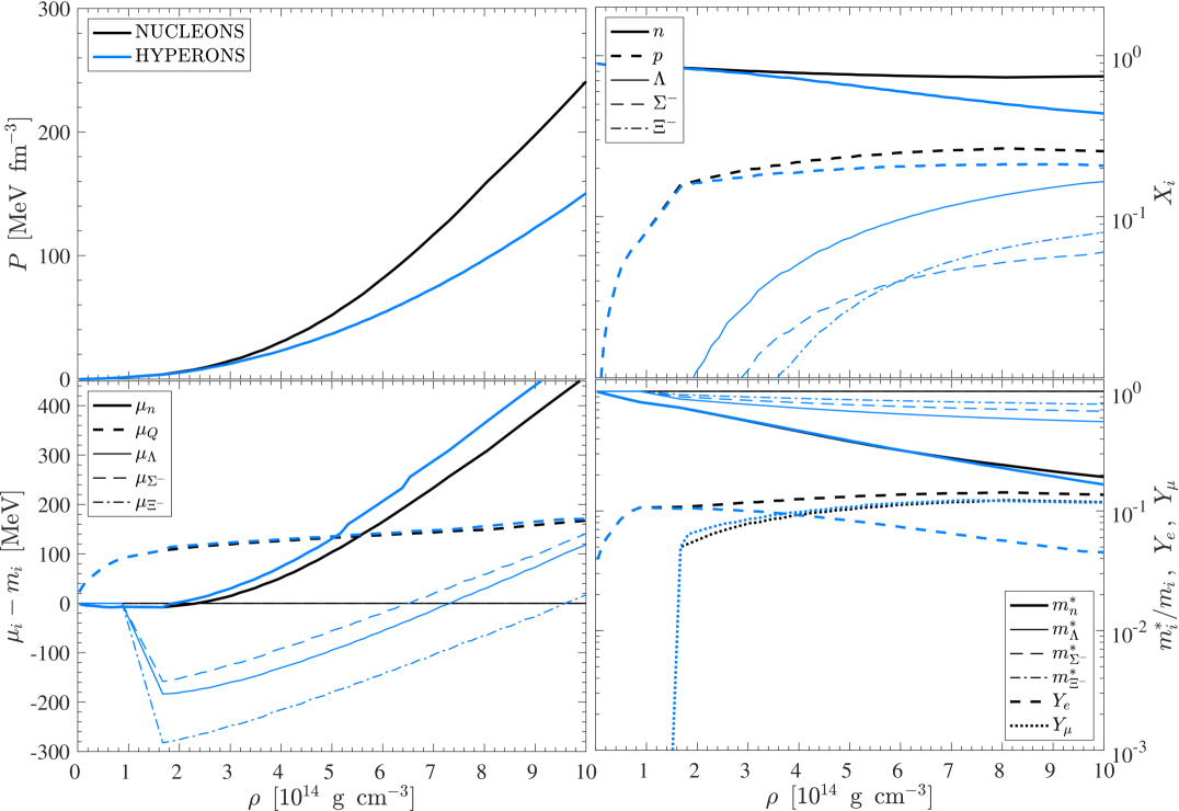
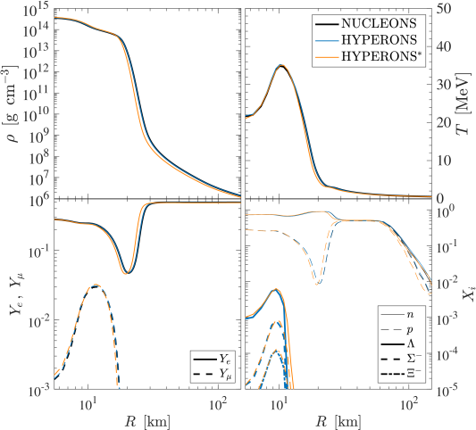
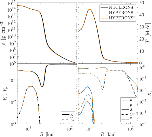
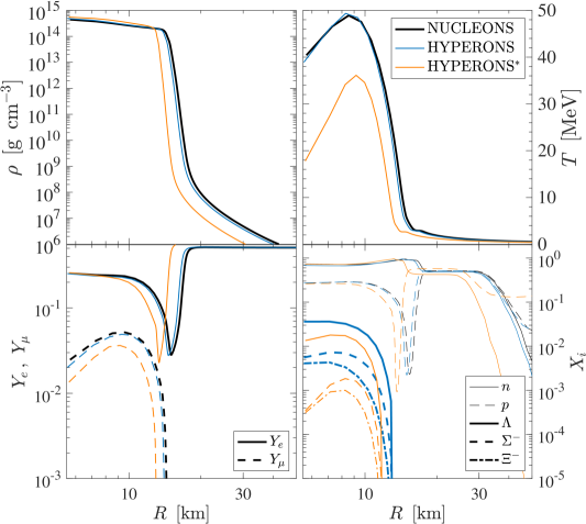
Figures 1 and 2 illustrate selected quantities of the NUCLEONS EOS (black lines) and HYPERONS EOS (blue lines) at certain conditions, at in Fig. 1 and at a constant entropy of in Fig. 2, both assuming -equilibrium. For both cases it becomes evident that the HYPERONS EOS is substantially softer at high densities than the NUCLEONS EOS, illustrated by the pressure in the upper left panels of Figs. 1 and 2. This is a consequence from the lower neutron abundance since the EOS is dominated by the neutron degeneracy at the high densities explored here (see therefore the hadron abundances in the upper right panels and note the generally low abundances222 In the case of particles with baryon number equal one, abundances and mass fractions are identical, defined through the partial densities with baryon density . of hyperons , and ). Note also the modified charge neutrality conditions in the presence of hyperons, illustrated via the electron and muon abundances, and , respectively, in the lower right panels, together with the density dependence of the effective masses gap equations (2.4).
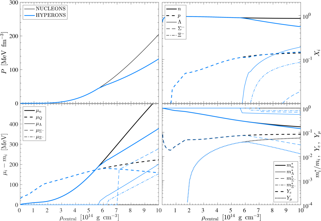
The assumption of -equilibrium results in the condition of equal chemical potentials for electrons and muons, , once the electron chemical potential exceeds the muon restmass, MeV, which was employed here for the calculation of the muon abundances. Note that this assumption differs from the conditions realized in the CCSN simulations. This discrepancy has been pointed out in Refs. [118, 19], that while , this condition can be reached only after more than 30 s post bounce in simulations of the PNS deleptonization and cooling, studied based on the DD2 relativistic mean field EOS, with density dependent meson-nucleon couplings [111]. As a consequence of this simplification applied here for the calculation of the muon EOS, the muon abundance is found to be significantly larger than what we find in the CCSN and PNS simulations, that will be discussed in Sec. 4 below.
The lower right panels in Figs. 1 and 2 also show the effective hadron masses, , relative to their vacuum values , from which it becomes evident that the neutron mass decreases most rapidly towards about 15% of its vacuum value at a density of slightly above g cm-3, whereas the effective mass of the is about 50% of its vacuum value at the same density. The corresponding chemical potentials, without rest masses , are shown in the lower left panels of Figs. 1 and 2. At zero temperature, hyperons are strictly suppressed when their effective chemical potentials, shown in the lower left panel in Fig. 1, are below their respective rest masses, while at finite temperature, shown in Fig. 2, this condition does not apply any longer.
4 Simulations of the PNS deleptonization with hyperons
For the simulations of the PNS deleptonization, the AGILE-BOLTZTRAN spherically symmetric general relativistic neutrino radiation hydrodynamics model is employed (c.f. Refs. [112, 113, 114, 115] and references therein). It is based on six-species Boltzmann neutrino transport and a complete set of weak interactions (the weak reactions used in the current study, including the references, are listed in Table 1 of ref. [116]). We distinguish between and (anti)neutrinos due to the inclusion of weak reactions involving muons and antimuons. These include the muonic charged current reactions, based on the full kinematics approach [117], as well as neutrino-(anti)muon inelastic scattering. For both of which we are following the implementation of ref. [118].
AGILE-BOLTZTRAN has a flexible EOS module that contains the Lattimer & Swesty Skyrme model [119] as well as the comprehensive RMF EOS catalogue of ref. [120]. The latter incorporates the modified nuclear statistic equilibrium (NSE) with several thousand nuclei [121], including excited state contributions, modelled via temperature dependent statistical weight factors for each nuclear species. The transition from the modified NSE to homogeneous nuclear matter is taken into account via a first-order phase transition construction where the nuclear states are suppressed through a geometric excluded volume approach (for alternative excluded volume functionals, c.f. ref. [122] and references therein). In ref. [120], the excluded volume parameter is chosen to result in the complete disappearance of all nuclei at nuclear saturation density. In the present study, we replace the supersaturation density phase of the DD2 RMF EOS [111, 120], with density-dependent meson-nucleon mean-field couplings, with the NUCLEONS and HYPERONS settings from FSU2H∗. We find that this approach, despite its ad hoc nature, results in a smooth transition. EOS contributions from electrons, positron and photons, as well as Coulomb contributions for the non-NSE regime, are implemented based on the routines of ref. [123].
The inclusion of the HYPERONS EOS is connected with the implementation of the associated hyperon degrees of freedom, , and , into the AGILE-BOLTZTRAN CCSN model. It concerns their abundances as well as the single particle properties such as the effective masses, the chemical potentials and the mean-field potentials, according to the underlying model as was discussed in Sec. 3. In particular, the latter will become relevant when implementing weak processes involving hyperons, which, for the present study, are being omitted as the simulation times are limited to when neutrinos still decouple at lower densities where no hyperons are abundant. This situation will change towards later times, when neutrinos start to decouple in the regions where hyperons are abundant, such that the inclusion of weak processes involving hyperons would influence the further deleptonization and cooling behaviour. Furthermore, the presence of hyperons modifies the charge-neutrality condition, with the negatively charged hyperons considered, i.e. . Note that despite their consistent treatment and implementation into the CCSN simulations, the heavier, neutral hyperons, and , and the positively charged hyperons, and , are neglected in the following discussions, as they are all strongly Boltzmann suppressed under the extremely neutron-rich conditions at highest densities encountered at the PNS interior, i.e. the following abundance hierarchy generally holds: as well as and .
With this enhanced EOS module setup, simulations of CCSN are launched from two progenitor models, with zero-age main sequence masses of 18 M⊙ and 25 M⊙, both from the stellar evolution series of ref. [124]. These stellar progenitors are being evolved through all CCSN phases self consistently. It is found that up to several 100 ms post bounce, the abundance of hyperons remains small, below 1%, and no impact could be observed, not on the overall dynamics nor on the neutrino heating and cooling rates. The neutrino signals are indistinguishable between NUCLEONS and HYPERONS.
The simulations with the NUCLEONS and HYPERONS EOS proceed identically.
Since neutrino-driven explosions cannot be obtained for such massive iron-core progenitors in spherically symmetric CCSN simulations, we follow closely the procedure outlined in ref. [7]. Therefore, the electronic charged current weak rates are being enhanced in the gain layer, which results in the continuous shock expansion and the onset of the CCSN explosion. Once the shock reaches a radius of about 1000 km, we switch back to the standard weak rates, following the later PNS deleptonization. A similar procedure has been employed in ref. [125] for a large sample of CCSN explosion models for various different progenitors at different metalicities.
| progenitor massa | EOS | |||||||||||
|---|---|---|---|---|---|---|---|---|---|---|---|---|
| M | M | M | km | |||||||||
| 18 | NUCLEONS | 1.543 | 1.435 | 14.18 | ||||||||
| 18 | HYPERONS | 1.558 | 1.450 | 14.09 | ||||||||
| 25 | NUCLEONS | 1.942 | 1.792 | 14.84 | ||||||||
| 25 | HYPERONS | 1.938 | 1.791 | 14.45 |
Notes.
a models from the stellar evolution series of ref. [124]
b Evaluated at g cm-3 at about 10 s post bounce
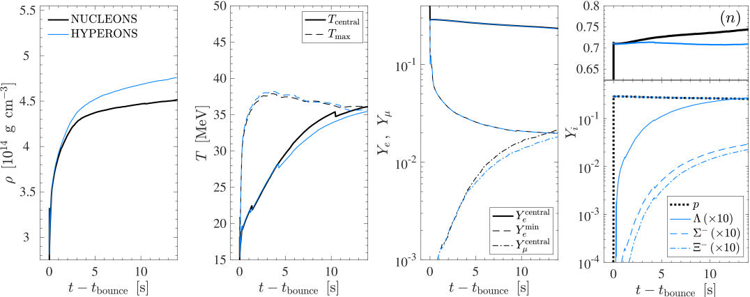
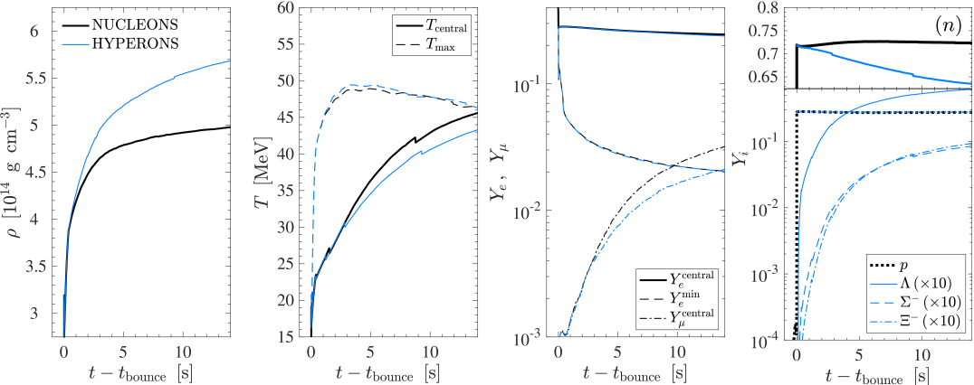
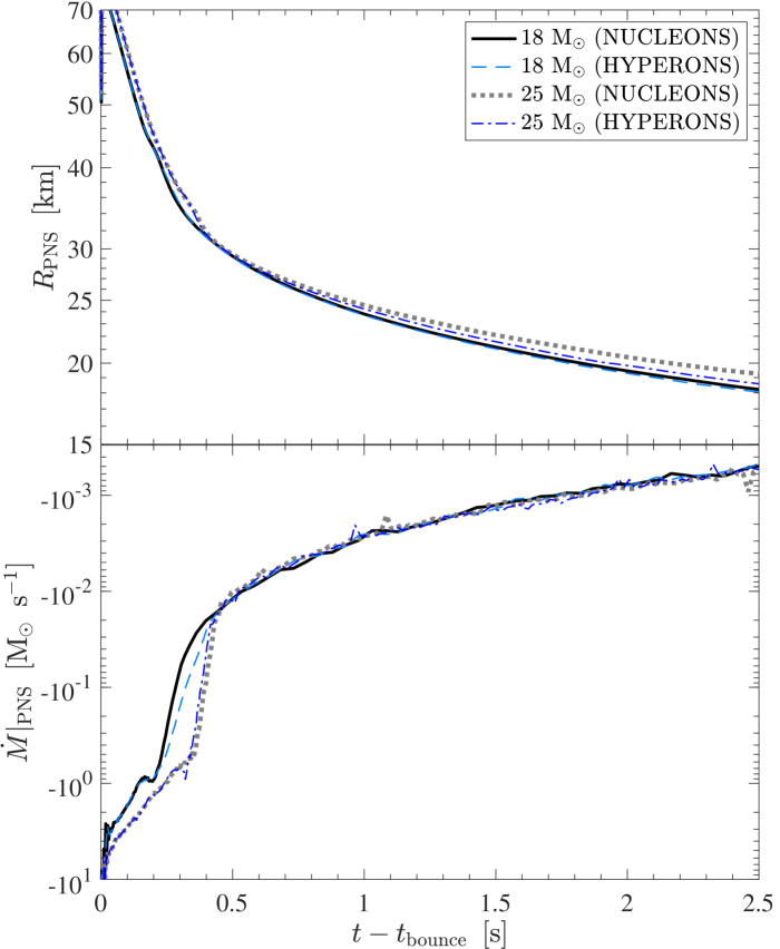
The post-bounce evolution of the four models is illustrated in Fig. 3, for 18 M⊙ and 25 M⊙ model in Figs. 3(a) and 3(b), respectively, distinguishing the NUCLEONS (black lines) and HYPERONS (blue lines) EOS. Once the supernova explosion proceeds with the revival of the shock, mass accretion onto the PNS surface ceases and the enclosed PNS baryon masses change only marginally. The latter is due to the ejection of the neutrino driven wind, initially on the order of M⊙ s-1 and later substantially lower with M⊙ s-1. The resulting PNS masses of the two sets of simulations are listed in Table 4, for both NUCLEONS and HYPERONS runs. These values are evaluated at the restmass density of g cm-3 at about 10 s post bounce. The larger PNS masses for the more massive progenitor are due to the higher post-bounce mass accretion rates for the 25 M⊙ models, in particular during the early post-bounce phase, i.e., before the shock revival, as is illustrated in the bottom panel of Fig. 4, showing the mass accretion rate , as well evaluated at g cm-3. The top panel illustrates the different PNS radii, , and their evolution for all simulations with the NUCLEONS and HYPERONS EOS under investigation, showing the slightly faster contraction of the HYPERONS PNS due to the softer supersaturation density behaviour.
Only after several seconds, in both simulations, differences due to the inclusion of hyperons arise. These differences are best seen by the evolution of the central densities, shown in the left panels of Figs. 3(a) and 3(b), where the simulations based on the HYPERONS EOS reach significantly higher values than the ones with NUCLEONS. This EOS softening is due to the continuous rise of the hyperon abundances for , and , shown in the right panels. Note that these hyperons are absent for the NUCLEONS simulations (black lines). The first hyperons which appear are ’s, due to the lowest mass (see Figs. 1 and 2), already at a density slightly in excess of nuclear saturation density, i.e. already during the early post-bounce evolution prior to the supernova explosion onset. However, the abundance of remains low, on the order of for the for 18 M⊙ model and for the for 25 M⊙ model. The latter reach higher abundances because of the generally higher densities and temperatures obtained at the central fluid elements in the simulations. Note therefore the different evolution of the central and maximum temperatures in Figs. 3(a) and 3(b). The abundances of the other hyperons, and , remain about one order of magnitude lower than those of , in both simulations.
Another difference between the runs with NUCLEONS and HYPERONS is the feedback to the nucleons. As was already discussed in Sec. 3, in particular the abundance of neutrons is reduced due to the appearance of , effectively replacing neutrons with ’s. This phenomenon is observed consistently in the CCSN simulations too. The neutron abundances are shown in the right panels of Figs. 3(a) and 3(b). The reduced neutron abundance in addition softens the high-density EOS, which is governed by neutrons with a dominating abundance of –. As a consequence of the different hadronic abundances, in order to obey the condition of charge neutrality, there is a feedback to the electron and muon abundances. In particular, the central muon abundance is reduced substantially for the massive 25 M⊙ model. Note also that the central muon abundance is substantially lower and that the central electron abundance is substantially higher than in the EOS discussion in Sec. 3, where -equilibrium was assumed. The observed difference of the electron and in particular the muon abundances are a consequence of the lower central temperatures obtained for the simulations based on the HYPERONS EOS (see Fig. 3), since the muons are produced thermally through the muonic charged current processes.
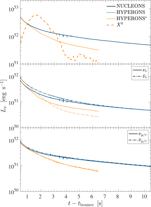
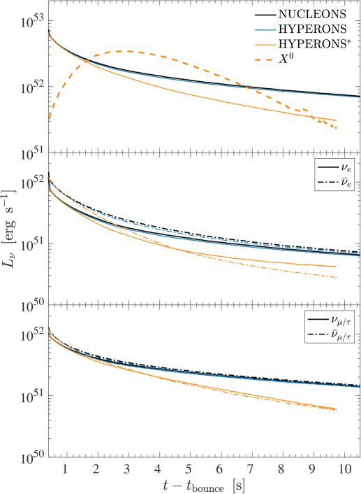
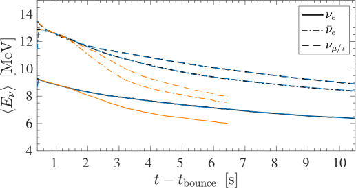
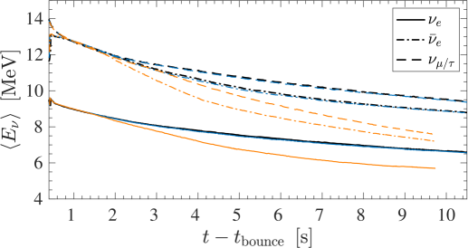
Despite the differences obtained at the PNS interior, structure and stability of the PNS are not affected by the presence of hyperons. This is partly related to the conditions for the appearance of hyperons, which in turn gives rise to finite hyperon abundances, in particular only at the very central fluid elements in the simulations. As a consequence, the locations of the neutrinospheres are not affected by the presence of hyperons and hence the neutrino luminosities and average energies are indistinguishable between the runs NUCLEONS and HYPERONS, for the intermediate-mass 18 M⊙ model, shown in Figs. 5(a) and 5(c), and high-mass 25 M⊙ model, shown in Figs. 5(b) and 5(d). The evolution of the neutrino luminosities and average energies shown in Fig. 5 are sampled in the co-moving frame of reference at a distance of 500 km.
5 Dark flavoured sectors during PNS deleptonization
The results including the dark flavoured sector are based on the same HYPERON EOS and will be henceforth denoted as HYPERONS∗, which will be discussed in this section. To investigate the impact of a dark flavoured sector in CCSN, we need to estimate the emissivity in the new channels. We assume that the emitted particles are massless (i.e. their mass is much smaller than ) and that the interactions are such that their mean free path is much larger than the radius of the PNS. These particles will then freely stream out of the PNS once they are produced in its core.
5.1 Dark flavoured emissivity
For concreteness, in the following we will focus on the emission of neutral dark bosons , such as an axion or dark photon, produced by the flavour-violating transition . This is parametrised by the following Lagrangians,
| (5.1) | |||||
| (5.2) |
where is the axion field and its decay constant and with strange and down quark fields denoted as and , respectively. is the field strength tensor of the dark photon and the energy scale associated to the UV completion of the effective Lagrangian (see ref. [97] for effective vectorial couplings of the dark photon and some UV completions), and and are dimensionless (effective) couplings. The main hadronic production mechanism in the PNS induced by Lagrangians (5.1) and (5.2) will then be , whereby decays involving heavier hyperons, such as , are suppressed by their lower abundances and neglected in the present analysis. Following ref. [82], the spectrum of the energy loss rate of the nuclear medium per unit volume, denoted as , with respect to the energy , in the PNS rest frame and induced by the process is given by the following expression,
| (5.3) |
with , is the energy of the with and are the relativistic Fermi-Dirac phase-space distribution functions of and . The information of the transition amplitude is encoded in , which is the decay rate of in vacuum,
| (5.4) |
with , where and are the vector and axial-vector baryonic couplings determined in ref. [82], and , where is the baryonic tensor coupling (further details can be found in ref. [83] and references therein).
The total emission rate can be estimated analytically by taking the nonrelativistic limit of the baryons, expanding to leading order in and neglecting the neutron’s Pauli blocking [82]. Expressed in terms of the emissivity, , one obtains the following result,
| (5.5) |
where we have re-expressed the decay width in terms of the lifetime, , and the branching fraction of the decay, BR. Adopting the classical upper limit of the emissivity, erg s-1 g-1, from SN1987A at the conditions of the PNS predicted at about 1 second post-bounce, one obtains,
| (5.6) |
This leads, for a characteristic abundance of 1%, to an upper limit of the branching fraction in the range of , which overestimates the conservative limit by a factor , which was obtained using the full expression in Eq. (5.3) and state-of-the-art spherically symmetric simulations reported in ref. [74]. Nevertheless, this upper bound is many orders of magnitude stronger than those that can be obtained from laboratory experiments, and, as was found in Refs. [82, 83], it leads to the strongest constraint on the axial couplings of the flavoured QCD axion and on the massless dark photon couplings. In addition, as discussed in ref. [83], in the case of processes one would still produce a too large emission in the deep trapping regime as the dark sector luminosity would stem from the last surface where ’s can coexist in equilibrium in the plasma and which corresponds to a region of high temperatures.
5.2 Impact of dark flavoured sector on PNS evolution
The non-relativistic emissivity (5.5) is implemented into the AGILE-BOLTZTRAN CCSN model as sink for the internal energy equation, following the implementation of dark boson losses of Refs. [126, 67]. Here, we use the literature branching ratios of for the intermediate-mass 18 M⊙ model and for the massive 25 M⊙ model, in accordance with ref. [83]. It results in enhanced cooling contributions in the domain where are abundant 333 These limits can be readily transformed in stringent limits on the flavoured QCD axion or massless dark photon described by the Lagrangians in (5.1) and (5.2). For example, in the QCD axion case with off-diagonal flavour couplings, the upper limit corresponds to the limit or (see Refs. [83] and [82] for details). . This is the case only at the innermost 15–20 km of the PNS, as is illustrated for both 18 M⊙ and 25 M⊙ models in Fig. 6 for two distinct post-bounce times of 1 s and 5 s, comparing the three setups NUCLEONS (black lines), HYPERONS (blue lines) and HYPERONS∗ (orange lines).
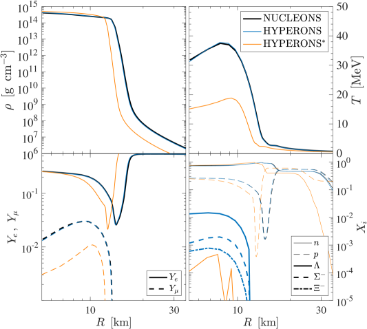
At around 1 s (top panels of Fig. 6), the abundance of reach as high as about at the very center for the 18 M⊙ model and about for the 25 M⊙ model. Going outwards in radius, the abundances rise, following the temperature profile, reaching their peak at around for the 18 M⊙ model and for the 25 M⊙ model. Figure 7 shows the corresponding dark particle emissivity (left scale) and luminosity (right scale) profiles. At around 1 s post bounce, dark sector emissivity and luminosity for the 18 M⊙ model exceed those of the 25 M⊙. Luminosities reach values of about erg for the former mode and about erg for the latter, which is also illustrated in the corresponding evolution of the dark sector luminosity in the top panels of Fig. 5. We attribute this to the larger branching ratio for the 18 M⊙ model, despite having slightly lower abundances and temperatures. Note also the sharp drop of the emissivities, after which the luminosities remain constant, which is due to the sudden drop of the abundance at around 13.75 km for the 18 M⊙ model and at around 14.5 km for the 25 M⊙ model, at 1 s post bounce. This is roughly to about one-half of saturation density, corresponding to conditions for the threshold for hyperons to exist within the HYPERON model EOS.
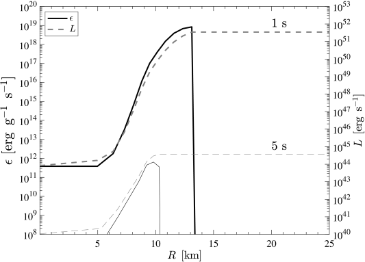
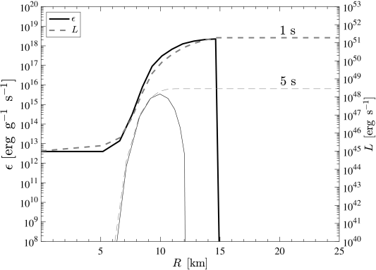
The situation changes during the ongoing PNS deleptonization with the inclusion of the additional losses due to dark boson emission. The luminosity evolution is illustrated in Fig. 5 (top panels), from where it becomes clear that the dark-boson losses dominate the cooling at around 1 s post bounce, for both intermediate-mass and high-mass models. However, the excess cooling results in the rapid drop of the PNS temperature, significantly faster than in the reference HYPERONS simulations (see the bottom panels of Fig. 6). Now, as the supernova interior features a lower temperature compared to the reference model without cooling, the feedback to the hyperon EOS is that the abundance is somewhat lower—note the strong temperature dependence of the hyperon EOS discussed in Sec. 3—depending on the timescale during the PNS deleptonization. As a consequence, at some point during the later evolution, the abundance will be too low for the process to still operate and the additional cooling due to emission ceases, featuring the continuous decrease of the luminosity; see the thick dashed lines in the top panels of Figs. 5(a) and 5(b). In a sense, the system self regulates it’s excess cooling, however, depending sensitively on the BR.
This is illustrated for the 5 s post-bounce curves in Fig. 7 such that the luminosities in Fig. 5 decrease below those of the total neutrinos and the later evolution will be determined by the neutrino losses. However, note that this is the case already at around 3 s post bounce for the intermediate-mass 18 M⊙ model, while only at around 7 s post bounce for the massive 25 M⊙ model. It is related to the generally higher temperatures and central densities for the latter model, featuring generally higher abundances of hyperons.
We note also the feedback from the excess cooling due to emission, namely the more rapid drop of the neutrino luminosities and average energies, for all flavours, during the PNS deleptonization phase that is dominated by cooling (see Fig. 5). We observe the reduction of the neutrino emission timescale by a factor of roughly two for both intermediate-mass and high-mass models.
6 Summary and conclusions
Novel hyperonic EOS are studied in simulations of CCSN in spherical symmetry. These are based on general relativistic neutrino radiation hydrodynamics, featuring six-species Boltzmann neutrino transport. Particular emphasis has been put on the role of hyperons, which have long been studied in the context of cold neutron stars, where it has been speculated that the super-saturation density EOS softens due to the appearance of these additional and heavy degrees of freedom. In the context of CCSN studies, hyperons have so far only been taken into account in failed CCSN explosion studies that result in the formation of black holes [26, 29, 30], however, based on hadronic EOS with a limited set of hyperons. The focus of the present article is on the long-term evolution of neutrino-driven CCSN explosions, i.e. the deleptonization and later cooling phases of the nascent PNS, based on hadronic EOS including a comprehensive set of hyperons that include, , and . The FSU2H∗ hyperon EOS employed in the present study is based on the RMF framework [103, 104] with meson-nucleon coupling constants selected to reproduce nuclear matter and finite nuclei properties, to fulfil certain constraints of high dense matter coming from heavy-ion collisions as well as to be consistent with the observation of massive 2 M⊙ pulsars.
The results differ from those reported in the comprehensive CCSN hyperon EOS study of ref. [127] in various ways. The largest difference arises due to the implementation of larger sample of hadronic states in the present paper. These modify the charge neutrality condition such that , which is the case in ref. [127] where no charged hyperons were considered. A second difference is related to the onset densities for the appearance of hyperons, which is the case at somewhat higher densities in ref. [127], and the abundance of hyperons is significantly higher than for the present HYPERONS EOS. In particular, in ref. [127] the abundance of hyperons exceeds those of the neutrons at high baryon densities on the order of , even at low temperatures on the order of –.
In the CCSN simulations, the appearance of hyperons leaves a negligible impact on both the PNS structure during the entire early post-bounce evolution prior to the supernova shock revival and subsequent explosion onset. The reason is related to the generally low abundance of hyperons. The high-density EOS is dominated by the protons and neutrons. This situation changes only after several seconds, during the long-term PNS deleptonization evolution, when the central density rises continuously such that also the abundances of hyperons increase. However, even for massive PNS, on the order of about 2 M⊙, the abundance of hyperons never exceeds more than few percent while the abundances of all heavier hyperons remain substantially lower, on the order of less than one percent. On the timescales considered here, on the order of several tens of seconds, the impact from the presence of hyperons on the PNS evolution remain negligible. CCSN observables, such as the neutrino signal, are hence insensitive to the composition at super-saturation density, explored in the present study within a RMF model and neglecting possible contributions to the weak interactions. In particular, the latter assumption becomes invalid once neutrinos start to decouple in the hyperon phase. This, however, has not been the case for the entire CCSN simulations under investigation.
The implementation of the hyperon in the CCSN simulations enables us to study the impact of a possible dark sector. These arise from the flavour-violating transition of strange quarks into down quarks, taken into account here from the decay of hyperon into neutron via the emission of dark bosonic degrees of freedom. Other decays, such as that of are neglected due to their generally low abundances under the conditions of high isospin asymmetry encountered at the interior of the PNS.
The excess cooling imposed by the inclusion of dark losses in the CCSN simulations results in a qualitative different evolution, in particular during the long-term PNS deleptonization phase when the abundance of hyperons reaches their maximum. It is assumed that these massless particles escape the star once upon production. Possible re-scattering is omitted, which is consistent with the small couplings to the dark sector we are considering (c.f. ref. [83]). As a consequence, the PNS deleptonizes on a shorter timescale due to the different thermal evolution. As a feedback, similar as has been reported for the case of axion cooling (c.f. Refs. [126, 63, 67]) in the case of light axions from QCD processes, we find that the neutrino emission timescale is reduced by roughly a factor of two. This is consistent with the argument of ref. [58], confirming both values of the branching ratios, for the low mass and for the high mass models, as limiting cases corresponding to the intermediate-mass and high-mass PNS models of about 1.6 M⊙ and 2.0 M⊙, respectively. We explore these two cases at the level of neutrino-driven CCSN explosions of 18 and 25 M⊙ progenitors from the stellar evolution series of ref. [124], which result in remnant PNS masses of about 1 .6 M⊙ and 2.0 M⊙ with lower central density and hence lower abundance for the former and the opposite for the latter models. We note here that the recent analysis at the level of the average -energy and the total -energy emitted, deduced from the KAM-II, IBM, BUST and LSD detections of SN1987A [128, 129], indicates that present standard core-collapse supernova models agree quantitatively with these measurements of the first few seconds of events while some tension remains with the late time events of Kam-II, IBM and BUST. The latter is due to generally short cooling timescales of all present long-term supernova simulations, including the PNS deleptonization and cooling phases. Note that considering the KAM-II data alone, current supernova models seemingly overestimate the detected average energy, including the late-time detection. If these finding will be confirmed, in particular also from future supernova neutrino detection of the next galactic events, this would potentially put certain constraints on the requirement of non-standard additional cooling agents, such as the losses explored in this work due to the presence of strange hadronic degrees of freedom.
It has to be emphasised that the entire analysis, both comparing nucleonic and hyperonic EOS in CCSN simulations as well as the impact of associated dark sector cooling, is entirely model EOS dependent. The present analysis of the impact of dark photon losses in CCSN is dominated by the phase space of and the neutron degeneracy, which in turn are determined by the underlying hyperonic model. EOS with a quantitative different high-density behaviour of the strange degrees of freedom, e.g., featuring a lower(higher) abundance of , will resemble also a lesser(stronger) impact on the excess dark cooling as is reported in the present article. All of these uncertainties can be related to the fact that the two-body and three-body interactions involving hyperons are poorly known. This is due to the fact that the available scattering data are still scarce and subject to quite large error bars, although promising results are becoming available from final-state interaction analyses and femtoscopy studies [44, 45, 46, 47, 48]. Also, data on hypernuclear structure can provide indirect information about the hyperon nuclear forces [49, 50, 51]. Moreover, advances can be anticipated on the experimental determination of two-body and three-body interactions involving hyperons and nucleons, e.g. at J-PARC, LHC or the future FAIR facility.
Another simplification applied here is related to the assumption of chemical equilibrium for strangeness imposing equal chemical potentials, e.g., of neutrons and hyperons. On the other hand, the CCSN timescales, e.g., weak interactions, mass accretion and diffusion, might be potentially on the same order of magnitude as the timescale for hyperons to appear, however, through weak processes. In other words, chemical equilibrium between strange and non-strange hadrons might not be fulfilled, similar as the condition of weak equilibrium is not fulfilled for muons for simulation times on the order of more than 30 s of the PNS deleptonization phase, as was shown in the Appendix of ref. [67]. This requires the implementation of non-equilibrium methods in order to solve for the problem of strangeness in CCSN, which we leave for future explorations.
Acknowledgments
We would like to thank Pok Man Lo for helpful comments and inspiring discussions. TF acknowledges support from the Polish National Science Centre (NCN) under grant number 2023/49/B/ST9/03941. JMC thanks MICINN for funding through the grant “DarkMaps” PID2022-142142NB-I00 and from the European Union through the grant “UNDARK” of the Widening participation and spreading excellence programme (project number 101159929). HK acknowledges support from the PRE2020-093558 Doctoral Grant of the spanish MCIN/AEI/10.13039/ 501100011033/. LT acknowledges support from the project CEX2020-001058-M (Unidades de Excelencia “María de Maeztu”) and PID2022-139427NB-I00, financed by the Spanish MCIN/ AEI/10.13039/501100011033/, as well as by the EU STRONG-2020 project, under the program H2020-INFRAIA-2018-1 grant agreement no. 824093, from the DFG through projects No. 315477589 - TRR 211 (Strong-interaction matter under extreme conditions), and from the Generalitat de Catalunya under contract 2021 SGR 171. All scientific computations were performed at the Wroclaw Centre for Scientific Computing and Networking (WCSS) under ’grant328’.
References
- [1] H.-Th. Janka, K. Langanke, A. Marek, G. Martínez-Pinedo and B. Müller, Theory of core-collapse supernovae, Phys. Rep. 442 (2007) 38 [ arXiv:0612072].
- [2] A. Mirizzi, I. Tamborra, H.-Th. Janka, N. Saviano, K. Scholberg, R. Bollig et al., Supernova neutrinos: production, oscillations and detection, Nuovo Cimento Rivista Serie 39 (2016) 1 [ arXiv:1508.00785].
- [3] A. Burrows and D. Vartanyan, Core-collapse supernova explosion theory, Nature 589 (2021) 29 [arXiv:2009.14157].
- [4] J. M. LeBlanc and J. R. Wilson, A Numerical Example of the Collapse of a Rotating Magnetized Star, Astrophys. J. 161 (1970) 541.
- [5] H. A. Bethe and J. R. Wilson, Revival of a stalled supernova shock by neutrino heating, Astrophys. J. 295 (1985) 14.
- [6] F. S. Kitaura, H.-Th. Janka and W. Hillebrandt, Explosions of O-Ne-Mg cores, the Crab supernova, and subluminous type II-P supernovae, Astron. Astrophys. 450 (2006) 345 [arXiv:0512065].
- [7] T. Fischer, S.C. Whitehouse, A. Mezzacappa, F. K. Thielemann and M. Liebendörfer, Protoneutron star evolution and the neutrino-driven wind in general relativistic neutrino radiation hydrodynamics simulations, Astron. Astrophys. 517 (2010) A80 [arXiv:0908.1871].
- [8] L. Hüdepohl, B. Müller, H.-Th. Janka, A. Marek and G.G. Raffelt, Neutrino Signal of Electron-Capture Supernovae from Core Collapse to Cooling, Phys. Rev. Lett. 104 (2010) 251101 [arXiv:0912.0260].
- [9] T. M. Tauris, N. Langer and P. Podsiadlowski, Ultra-stripped supernovae: progenitors and fate, MNRAS 451 (2015) 2123 [arXiv:1505.00270].
- [10] K. De, M. M. Kasliwal, E. O. Ofek, T. J. Moriya, J. Burke, Y. Cao et al., A hot and fast ultra-stripped supernova that likely formed a compact neutron star binary, Science 362 (2018) 201 [arXiv:1810.05181].
- [11] B. Müller, D. W. Gay, A. Heger, T. M. Tauris and S. A. Sim, Multidimensional simulations of ultrastripped supernovae to shock breakout, MNRAS 479 (2018) 3675 [arXiv:1803.03388].
- [12] B. Müller, T. M. Tauris, A. Heger, P. Banerjee, Y.-Z. Qian, J. Powell et al., Three-dimensional simulations of neutrino-driven core-collapse supernovae from low-mass single and binary star progenitors, MNRAS 484 (2019) 3307 [arXiv:1811.05483].
- [13] T. Ertl, S.E. Woosley, T. Sukhbold and H.-Th. Janka, The Explosion of Helium Stars Evolved with Mass Loss, Astrophys. J. 890 (2020) 51 [arXiv:1910.01641].
- [14] G. Stockinger, H.-Th. Janka, D. Kresse, T. Melson, T. Ertl, M. Gabler et al., Three-dimensional models of core-collapse supernovae from low-mass progenitors with implications for Crab, MNRAS 496 (2020) 2039 [arXiv:2005.02420].
- [15] T. Wang and A. Burrows, Supernova Explosions of the Lowest-mass Massive Star Progenitors, Astrophys. J. 969 (2024) 74 [arXiv:2405.06024].
- [16] I. Sagert, T. Fischer, M. Hempel, G. Pagliara, J. Schaffner-Bielich, A. Mezzacappa et al., Signals of the QCD Phase Transition in Core-Collapse Supernovae, Phys. Rev. Lett. 102 (2009) 081101 [arXiv:0809.4225].
- [17] T. Fischer, N.-U. F. Bastian, M.-R. Wu, P. Baklanov, E. Sorokina, S. Blinnikov et al., Quark deconfinement as a supernova explosion engine for massive blue supergiant stars, Nature Astronomy 2 (2018) 980 [arXiv:1712.08788].
- [18] S. Zha, E. P. O’Connor, M.-c. Chu, L.-M. Lin and S.M. Couch, Gravitational-wave Signature of a First-order Quantum Chromodynamics Phase Transition in Core-Collapse Supernovae, Phys. Rev. Lett. 125 (2020) 051102 [arXiv:2007.04716].
- [19] T. Fischer, QCD phase transition drives supernova explosion of a very massive star, Eur. Phys. J. A 57 (2021) 270 [arXiv:2108.00196].
- [20] T. Kuroda, T. Fischer, T. Takiwaki and K. Kotake, Core-collapse Supernova Simulations and the Formation of Neutron Stars, Hybrid Stars, and Black Holes, Astrophys. J. 924 (2022) 38 [arXiv:2109.01508].
- [21] N. Khosravi Largani, T. Fischer and N.-U. F. Bastian, Constraining the Onset Density for the QCD Phase Transition with the Neutrino Signal from Core-collapse Supernovae, Astrophys. J. 964 (2024) 143 [arXiv:2304.12316].
- [22] T. Kuroda and M. Shibata, Spontaneous scalarization as a new core-collapse supernova mechanism and its multimessenger signals, Phys. Rev. D 107 (2023) 103025 [arXiv:2302.09853].
- [23] T. Fischer, N.-U. F. Bastian, D. Blaschke, M. Cierniak, M. Hempel, T. Klähn et al., The State of Matter in Simulations of Core-Collapse supernovae—Reflections and Recent Developments, Publications of the Astronomical society of Australia 34 (2017) e067 [arXiv:1711.07411].
- [24] A. Bauswein, N.-U. F. Bastian, D.B. Blaschke, K. Chatziioannou, J.A . Clark, T. Fischer et al., Identifying a First-Order Phase Transition in Neutron-Star Mergers through Gravitational Waves, Phys. Rev. Lett. 122 (2019) 061102 [arXiv:1809.01116].
- [25] E. R. Most, L. J. Papenfort, V. Dexheimer, M. Hanauske, S. Schramm, H. Stöcker et al., Signatures of Quark-Hadron Phase Transitions in General-Relativistic Neutron-Star Mergers, Phys. Rev. Lett. 122 (2019) 061101 [arXiv:1807.03684].
- [26] K. Sumiyoshi, C. Ishizuka, A. Ohnishi, S. Yamada and H. Suzuki, Emergence of Hyperons in Failed Supernovae: Trigger of the Black Hole Formation, Astrophys. J. 690 (2009) L43 [arXiv:0811.4237].
- [27] T. Fischer, S. C. Whitehouse, A. Mezzacappa, F.-K. Thielemann and M. Liebendörfer, The neutrino signal from protoneutron star accretion and black hole formation, Astron. Astrophys. 499 (2009) 1 [arXiv:0809.5129].
- [28] E. O’Connor and C.D. Ott, Black Hole Formation in Failing Core-Collapse Supernovae, Astrophys. J. 730 (2011) 70 [arXiv:1010.5550].
- [29] K. Nakazato, S. Furusawa, K. Sumiyoshi, A. Ohnishi, S. Yamada and H. Suzuki, Hyperon Matter and Black Hole Formation in Failed Supernovae, Astrophys. J. 745 (2012) 197 [arXiv:1111.2900].
- [30] P. Char, S. Banik and D. Bandyopadhyay, A Comparative Study of Hyperon Equations of State in Supernova Simulations, Astrophys. J. 809 (2015) 116 [arXiv:1508.01854].
- [31] G.F. Burgio and A.F. Fantina, Nuclear equation of state for compact stars and supernovae, in The Physics and Astrophysics of Neutron Stars, pp. 255–335, Springer International Publishing (2018).
- [32] L. Tolos and L. Fabbietti, Strangeness in Nuclei and Neutron Stars, Prog. Part. Nucl. Phys. 112 (2020) 103770 [arXiv:2002.09223].
- [33] G.F. Burgio, H.J. Schulze, I. Vidana and J.B. Wei, Neutron stars and the nuclear equation of state, Prog. Part. Nucl. Phys. 120 (2021) 103879 [arXiv:2105.03747].
- [34] MUSES collaboration, Theoretical and experimental constraints for the equation of state of dense and hot matter, Living Rev. Rel. 27 (2024) 3 [arXiv:2303.17021].
- [35] P. Demorest, T. Pennucci, S. Ransom, M. Roberts and J. Hessels, Shapiro delay measurement of a two solar mass neutron star, Nature 467 (2010) 1081. [arXiv:1010.5788].
- [36] J. Antoniadis, P.C.C. Freire, N. Wex, T.M. Tauris, R.S. Lynch, M.H. van Kerkwijk et al., A Massive Pulsar in a Compact Relativistic Binary, Science 340 (2013) 448 [arXiv:1304.6875].
- [37] E. Fonseca, H.T. Cromartie, T.T. Pennucci, P.S. Ray, A.Y. Kirichenko, S.M. Ransom et al., Refined Mass and Geometric Measurements of the High-mass PSR J0740+6620, Astrophys. J. 915 (2021) L12 [arXiv:2104.00880].
- [38] NANOGrav collaboration, Relativistic Shapiro delay measurements of an extremely massive millisecond pulsar, Nature Astron. 4 (2019) 72 [arXiv:1904.06759].
- [39] R.W. Romani, D. Kandel, A.V. Filippenko, T.G. Brink and W. Zheng, PSR J09520607: The Fastest and Heaviest Known Galactic Neutron Star, Astrophys. J. Lett. 934 (2022) L17 [arXiv:2207.05124].
- [40] S. Petschauer, J. Haidenbauer, N. Kaiser, U.-G. Meißner and W. Weise, Hyperon-nuclear interactions from SU(3) chiral effective field theory, Front. in Phys. 8 (2020) 12 [arXiv:2002.00424].
- [41] P. M. Lo, Density of states of a coupled-channel system, Phys. Rev. D 102 (2020) 034038 [arXiv:2007.03392].
- [42] J. Cleymans, P. M. Lo, K. Redlich and N. Sharma, Multiplicity dependence of (multi)strange baryons in the canonical ensemble with phase shift corrections, Phys. Rev. C 103 (2021) 014904 [arXiv:2009.04844].
- [43] P. M. Lo, Thermal study of a coupled-channel system: a brief review, European Physical Journal A 57 (2021) 60.
- [44] CLAS collaboration, Improved Elastic Scattering Cross Sections Between 0.9 and 2.0 GeV/c and Connections to the Neutron Star Equation of State, Phys. Rev. Lett. 127 (2021) 272303 [arXiv:2108.03134].
- [45] J-PARC E40 collaboration, Measurement of the differential cross sections of the elastic scattering in momentum range 470 to 850 MeV/c, Phys. Rev. C 104 (2021) 045204 [arXiv:2104.13608].
- [46] J-PARC E40 collaboration, Precise measurement of differential cross sections of the reaction in momentum range 470-650 MeV, Phys. Rev. Lett. 128 (2022) 072501 [arXiv:2111.14277].
- [47] J-PARC E40 collaboration, Measurement of differential cross sections for +p elastic scattering in the momentum range 0.44–0.80 GeV/c, PTEP 2022 (2022) 093D01 [arXiv:2203.08393].
- [48] L. Fabbietti, V. Mantovani Sarti and O. Vazquez Doce, Study of the Strong Interaction Among Hadrons with Correlations at the LHC, Ann. Rev. Nucl. Part. Sci. 71 (2021) 377 [arXiv:2012.09806].
- [49] A. Feliciello and T. Nagae, Experimental review of hypernuclear physics: recent achievements and future perspectives, Rept. Prog. Phys. 78 (2015) 096301.
- [50] H. Tamura et al., Gamma-ray spectroscopy of hypernuclei - present and future, Nucl. Phys. A 914 (2013) 99.
- [51] A. Gal, E.V. Hungerford and D.J. Millener, Strangeness in nuclear physics, Rev. Mod. Phys. 88 (2016) 035004 [arXiv:1605.00557].
- [52] A. R. Raduta, F. Nacu and M. Oertel, Equations of state for hot neutron stars, Eur. Phys. J. A 57 (2021) 329 [arXiv:2109.00251].
- [53] A. R. Raduta, Equations of state for hot neutron stars-II. The role of exotic particle degrees of freedom, Eur. Phys. J. A 58 (2022) 115 [arXiv:2205.03177].
- [54] M. Oertel, M. Hempel, T. Klähn and S. Typel, Equations of state for supernovae and compact stars, Rev. Mod. Phys. 89 (2017) 015007 [arXiv:1610.03361].
- [55] V. Dexheimer, M. Mancini, M. Oertel, C. Providência, L. Tolos and S. Typel, Quick Guides for Use of the CompOSE Data Base, Particles 5 (2022) 346 [arXiv:2311.04715].
- [56] CompOSE Core Team collaboration, CompOSE Reference Manual, Eur. Phys. J. A 58 (2022) 221 [arXiv:2203.03209].
- [57] G. G. Raffelt and D. Seckel, Bounds on Exotic Particle Interactions from SN 1987a, Phys. Rev. Lett. 60 (1988) 1793.
- [58] G. G. Raffelt, Stars as laboratories for fundamental physics : the astrophysics of neutrinos, axions, and other weakly interacting particles (1996).
- [59] M. S. Turner, Axions from SN 1987a, Phys. Rev. Lett. 60 (1988) 1797.
- [60] R. Mayle, J.R. Wilson, J.R. Ellis, K.A. Olive, D.N. Schramm and G. Steigman, Constraints on Axions from SN 1987a, Phys. Lett. B 203 (1988) 188.
- [61] A. Burrows, M. S. Turner and R. Brinkmann, Axions and SN 1987a, Phys. Rev. D 39 (1989) 1020.
- [62] A. Burrows, M. Ressell and M. S. Turner, Axions and SN1987A: Axion trapping, Phys. Rev. D 42 (1990) 3297.
- [63] P. Carenza, T. Fischer, M. Giannotti, G. Guo, G. Martínez-Pinedo and A. Mirizzi, Improved axion emissivity from a supernova via nucleon-nucleon bremsstrahlung, JCAP 10 (2019) 016 [arXiv:1906.11844].
- [64] K. Choi, H. J. Kim, H. Seong and C. S. Shin, Axion emission from supernova with axion-pion-nucleon contact interaction, JHEP 02 (2022) 143 [arXiv:2110.01972].
- [65] L. Di Luzio, M. Giannotti, E. Nardi and L. Visinelli, The landscape of QCD axion models, Phys. Rept. 870 (2020) 1 [arXiv:2003.01100].
- [66] P. Carenza, B. Fore, M. Giannotti, A. Mirizzi and S. Reddy, Enhanced Supernova Axion Emission and its Implications, Phys. Rev. Lett.126 (2021) 071102 [arXiv:2010.02943].
- [67] T. Fischer, P. Carenza, B. Fore, M. Giannotti, A. Mirizzi and S. Reddy, Observable signatures of enhanced axion emission from protoneutron stars, Phys. Rev. D 104 (2021) 103012 [arXiv:2108.13726].
- [68] E. Rrapaj and S. Reddy, Nucleon-nucleon bremsstrahlung of dark gauge bosons and revised supernova constraints, Phys. Rev. C 94 (2016) 045805 [arXiv:1511.09136].
- [69] J. H. Chang, R. Essig and S. D. McDermott, Supernova 1987A Constraints on Sub-GeV Dark Sectors, Millicharged Particles, the QCD Axion, and an Axion-like Particle, JHEP 09 (2018) 051 [arXiv:1803.00993].
- [70] F. Calore, P. Carenza, M. Giannotti, J. Jaeckel, G. Lucente and A. Mirizzi, Supernova bounds on axionlike particles coupled with nucleons and electrons, Phys. Rev. D 104 (2021) 043016 [arXiv:2107.02186].
- [71] S. Balaji, P.S.B. Dev, J. Silk and Y. Zhang, Improved stellar limits on a light CP-even scalar, JCAP 2022 (2022) 024 [arXiv:2205.01669].
- [72] A. Lella, P. Carenza, G. Lucente, M. Giannotti and A. Mirizzi, Protoneutron stars as cosmic factories for massive axionlike particles, Phys. Rev. D 107 (2023) 103017 [arXiv:2211.13760].
- [73] C. A. Manzari, J. M. Camalich, J. Spinner and R. Ziegler, Supernova limits on muonic dark forces, Phys. Rev. D 108 (2023) 103020 [arXiv:2307.03143].
- [74] R. Bollig, W. DeRocco, P. W. Graham and H.-Th. Janka, Muons in supernovae: implications for the axion-muon coupling, Phys. Rev. Lett. 125 (2020) 051104 [arXiv:2005.07141].
- [75] L. Calibbi, D. Redigolo, R. Ziegler and J. Zupan, Looking forward to lepton-flavor-violating ALPs, JHEP 09 (2021) 173 [arXiv:2006.04795].
- [76] D. Croon, G. Elor, R. K. Leane and S. D. McDermott, Supernova Muons: New Constraints on ’ Bosons, Axions and ALPs, JHEP 01 (2021) 107 [arXiv:2006.13942].
- [77] A. Caputo, G.G. Raffelt and E. Vitagliano, Muonic boson limits: Supernova redux, Phys. Rev. D 105 (2022) 035022 [arXiv:2109.03244].
- [78] M. S. Turner, Dirac neutrinos and SN1987A, Phys. Rev. D 45 (1992) 1066.
- [79] G. G. Raffelt and D. Seckel, A selfconsistent approach to neutral current processes in supernova cores, Phys. Rev. D 52 (1995) 1780 [arXiv:9312019].
- [80] W. Keil, H.-Th. Janka, D. N. Schramm, G. Sigl, M. S. Turner and J. R. Ellis, A Fresh look at axions and SN-1987A, Phys. Rev. D 56 (1997) 2419 [arXiv:astro-ph/9612222].
- [81] C. S. Shin and S. Yun, Dark gauge boson emission from supernova pions, Phys. Rev. D 108 (2023) 055014 [arXiv:2211.15677].
- [82] J. M. Camalich, M. Pospelov, P. N. H. Vuong, R. Ziegler and J. Zupan, Quark Flavor Phenomenology of the QCD Axion, Phys. Rev. D 102 (2020) 015023 [arXiv:2002.04623].
- [83] J. M. Camalich, J. Terol-Calvo, L. Tolos and R. Ziegler, Supernova Constraints on Dark Flavored Sectors, Phys. Rev. D 103 (2021) L121301 [arXiv:2012.11632].
- [84] G. Alonso-Álvarez, G. Elor, M. Escudero, B. Fornal, B. Grinstein and J.M. Camalich, Strange physics of dark baryons, Phys. Rev. D 105 (2022) 115005 [arXiv:2111.12712].
- [85] M. Cavan-Piton, D. Guadagnoli, M. Oertel, H. Seong and L. Vittorio, Axion emission from strange matter in core-collapse SNe, arXiv:2401.10979.
- [86] J. F. Kamenik and C. Smith, FCNC portals to the dark sector, JHEP 03 (2012) 090 [arXiv:1111.6402].
- [87] E. Goudzovski et al., New physics searches at kaon and hyperon factories, Rept. Prog. Phys. 86 (2023) 016201 [arXiv:2201.07805].
- [88] A. Davidson and K. C. Wali, Minimal flavor unifications via multigenerational Pecci-Quinn symmetry, Phys. Rev. Lett. 48 (1982), 11
- [89] F. Wilczek, Axions and Family Symmetry Breaking, Phys. Rev. Lett. 49 (1982) 1549.
- [90] J. L. Feng, T. Moroi, H. Murayama and E. Schnapka, Third generation familons, b factories, and neutrino cosmology, Phys. Rev. D57 (1998) 5875 [arXiv:9709411].
- [91] L. Calibbi, F. Goertz, D. Redigolo, R. Ziegler and J. Zupan, Minimal axion model from flavor, Phys. Rev. D95 (2017) 095009 [arXiv:1612.08040].
- [92] Y. Ema, K. Hamaguchi, T. Moroi and K. Nakayama, Flaxion: a minimal extension to solve puzzles in the standard model, JHEP 01 (2017) 096 [arXiv:1612.05492].
- [93] L. Di Luzio, A.W.M. Guerrera, X.P. Díaz and S. Rigolin, On the IR/UV flavour connection in non-universal axion models, JHEP 06 (2023) 046 [arXiv:2304.04643].
- [94] B. Holdom, Two U(1)’s and Epsilon Charge Shifts, Phys. Lett. B 166 (1986) 196.
- [95] B. A. Dobrescu, Massless gauge bosons other than the photon, Phys. Rev. Lett. 94 (2005) 151802 [arXiv:0411004].
- [96] E. Gabrielli, B. Mele, M. Raidal and E. Venturini, FCNC decays of standard model fermions into a dark photon, Phys. Rev. D 94 (2016) 115013 [arXiv:1607.05928].
- [97] J. F. Eguren, S. Klingel, E. Stamou, M. Tabet and R. Ziegler, Flavor phenomenology of light dark vectors, JHEP 08 (2024) 111 [arXiv:2405.00108].
- [98] G. Elor, M. Escudero and A. Nelson, Baryogenesis and Dark Matter from Mesons, Phys. Rev. D 99 (2019) 035031 [arXiv:1810.00880].
- [99] T. Bringmann, J. M. Cline and J. M. Cornell, Baryogenesis from neutron-dark matter oscillations, Phys. Rev. D 99 (2019) 035024 [arXiv:1810.08215].
- [100] B. Fornal and B. Grinstein, Dark Matter Interpretation of the Neutron Decay Anomaly, Phys. Rev. Lett. 120 (2018) 191801 [arXiv:1801.01124].
- [101] L. Tolos, M. Centelles and A. Ramos, Equation of State for Nucleonic and Hyperonic Neutron Stars with Mass and Radius Constraints, Astrophys. J. 834 (2017) 3 [arXiv:1610.00919].
- [102] L. Tolos, M. Centelles and A. Ramos, The Equation of State for the Nucleonic and Hyperonic Core of Neutron Stars, Publ. Astron. Soc. Austral. 34 (2017) e065 [arXiv:1708.08681].
- [103] H. Kochankovski, A. Ramos and L. Tolos, Equation of state for hot hyperonic neutron star matter, Mon. Not. Roy. Astron. Soc. 517 (2022) 507 [arXiv:2206.11266].
- [104] H. Kochankovski, A. Ramos and L. Tolos, Hyperonic uncertainties in neutron stars, mergers, and supernovae, MNRAS 528 (2024) 2629 [arXiv:2309.14879].
- [105] S. Navas, et al. (Particle Data Group collaboration), Review of particle physics, Phys. Rev. D 110 (2024) 030001
- [106] LIGO Scientific, Virgo collaboration, GW170817: Observation of Gravitational Waves from a Binary Neutron Star Inspiral, Phys. Rev. Lett. 119 (2017) 161101 [arXiv:1710.05832].
- [107] M. C. Miller, F. K. Lamb, A. J. Dittmann, S. Bogdanov, Z. Arzoumanian, K. C. Gendreau et al., PSR J0030+0451 Mass and Radius from NICER Data and Implications for the Properties of Neutron Star Matter, Astrophys. J. 887 (2019) L24 [arXiv:1912.05705].
- [108] A. V. Bilous, A. L. Watts, A.K. Harding, T.E. Riley, Z. Arzoumanian, S. Bogdanov et al., A NICER View of PSR J0030+0451: Evidence for a Global-scale Multipolar Magnetic Field, Astrophys. J. 887 (2019) L23 [arXiv:1912.05704].
- [109] M. C. Miller, F. K. Lamb, A. J. Dittmann, S. Bogdanov, Z. Arzoumanian, K.C. Gendreau et al., The Radius of PSR J0740+6620 from NICER and XMM-Newton Data, Astrophys. J. 918 (2021) L28 [arXiv:2105.06979].
- [110] T. E. Riley, A. L. Watts, P. S. Ray, S. Bogdanov, S. Guillot, S. M. Morsink et al., A NICER View of the Massive Pulsar PSR J0740+6620 Informed by Radio Timing and XMM-Newton Spectroscopy, Astrophys. J. 918 (2021) L27 [arXiv:2105.06980].
- [111] S. Typel, G. Röpke, T. Klähn, D. Blaschke and H.H. Wolter, Composition and thermodynamics of nuclear matter with light clusters, Phys. Rev. C 81 (2010) 015803 [arXiv:0908.2344].
- [112] A. Mezzacappa and S. W. Bruenn, Type II supernovae and Boltzmann neutrino transport - The infall phase, Astrophys. J. 405 (1993) 637.
- [113] A. Mezzacappa and S. W. Bruenn, A numerical method for solving the neutrino Boltzmann equation coupled to spherically symmetric stellar core collapse, Astrophys. J. 405 (1993) 669.
- [114] A. Mezzacappa and S. W. Bruenn, Stellar core collapse - A Boltzmann treatment of neutrino-electron scattering, Astrophys. J. 410 (1993) 740.
- [115] M. Liebendörfer, O. E. B. Messer, A. Mezzacappa, S. W. Bruenn, C. Y. Cardall and F.-K. Thielemann, A Finite Difference Representation of Neutrino Radiation Hydrodynamics in Spherically Symmetric General Relativistic Spacetime, Astrophys. J. Suppl. 150 (2004) 263 [arXiv:0207036].
- [116] T. Fischer, G. Guo, A. A. Dzhioev, G. Martínez-Pinedo, M.-R. Wu, A. Lohs et al., Neutrino signal from proto-neutron star evolution: Effects of opacities from charged-current-neutrino interactions and inverse neutron decay, Phys. Rev. C 101 (2020) 025804 [arXiv:1804.10890].
- [117] G. Guo, G. Martínez-Pinedo, A. Lohs and T. Fischer, Charged-current muonic reactions in core-collapse supernovae, Phys. Rev. D 102 (2020) 023037 [arXiv:2006.12051].
- [118] T. Fischer, G. Guo, G. Martínez-Pinedo, M. Liebendörfer and A. Mezzacappa, Muonization of supernova matter, Phys. Rev. D 102 (2020) 123001 [arXiv:2008.13628].
- [119] J. M. Lattimer and F. Swesty, A generalized equation of state for hot, dense matter, Nuclear Physics A 535 (1991) 331.
- [120] M. Hempel, T. Fischer, J. Schaffner-Bielich and M. Liebendörfer, New Equations of State in Simulations of Core-collapse Supernovae, Astrophys. J. 748 (2012) 70 [arXiv:1108.0848].
- [121] M. Hempel and J. Schaffner-Bielich, A statistical model for a complete supernova equation of state, Nucl. Phys. A 837 (2010) 210 [arXiv:0911.4073].
- [122] T. Fischer, Constraining the supersaturation density equation of state from core-collapse supernova simulations?. Excluded volume extension of the baryons, European Physical Journal A 52 (2016) 54 [arXiv:1604.01629].
- [123] F. X. Timmes and D. Arnett, The Accuracy, Consistency, and Speed of Five Equations of State for Stellar Hydrodynamics, Astrophys. J. Suppl. 125 (1999) 277.
- [124] S. E. Woosley, A. Heger and T. A. Weaver, The evolution and explosion of massive stars, Rev. Mod. Phys. 74 (2002) 1015.
- [125] F. P. Jost, M. Molero, G. Navó, A. Arcones, M. Obergaulinger and F. Matteucci, Neutrino-driven Core-collapse Supernova Yields in Galactic Chemical Evolution, arXiv e-prints (2024) arXiv:2407.14319 [arXiv:2407.14319].
- [126] T. Fischer, S. Chakraborty, M. Giannotti, A. Mirizzi, A. Payez and A. Ringwald, Probing axions with the neutrino signal from the next Galactic supernova, Phys. Rev. D 94 (2016) 085012 [arXiv:1605.08780].
- [127] S. Banik, M. Hempel and D. Bandyopadhyay, New Hyperon Equations of State for Supernovae and Neutron Stars in Density-dependent Hadron Field Theory, Astrophys. J. Suppl. 214 (2014) 22 [arXiv:1404.6173].
- [128] D. F. G. Fiorillo, M Heinlein, H.-Th. Janka, G. Raffelt, E. Vitagliano, R. Bollig, Supernova simulations confront SN 1987A neutrinos, Phys. Rev. D 108 (2023) 083040 [arXiv:2308.01403].
- [129] S. W. Li, J. F. Beacom, L. F. Roberts,F. Capozzi Old data, new forensics: The first second of SN 1987A neutrino emission, Phys. Rev. D 109 (2024) 083025 [arXiv:2306.08024].