Hyperplane Distance Depth^††thanks: This work is funded in part by the Natural Sciences and Engineering Research Council of Canada (NSERC).

By Definition 9, the median is a point that minimizes the sum of the distances to all possible points passing through each point in $P$. Therefore, $H_{P}=P$. Consequently, the HDD median is equivalent to the usual definition of median in a one-dimensional space.

The distance function ${d_{h_{i}}(q)}$ from a query point $q$ to the hyperplane $h_{i}$ is convex. Any non-negative linear combination of convex functions is convex. Therefore, the HDD function $\sum_{h_{i}\in H_{P}}{d_{h_{i}}(q)}=D_{P}(q)$ is convex over $q$.

The distance from the point $q\in\mathbb{R}^{d}$ to a hyperplane $h_{i}$ is equal to ${d_{h_{i}}(q)}=\frac{|{w_{i}}.q+{b_{i}}|}{\|{w_{i}}\|}$ where $w_{i}$ and $b_{i}$ are the hyperplane’s normal vector and the offset respectively. Therefore, the HDD of the point $q$ is equal to

$$D_{P}(q)=\sum_{h_{i}\in H_{P}}{d_{h_{i}}(q)}=\sum_{h_{i}\in H_{P}}\frac{|{w_{i}}.q+{b_{i}}|}{\|{w_{i}}\|}$$

(2)

Depending on the position of $q$ with respect to $h_{i}$, ${d_{h_{i}}(q)}=\frac{|{w_{i}}.q+{b_{i}}|}{\|{w_{i}}\|}$ can be equal to $+\frac{{w_{i}}.q+{b_{i}}}{\|{w_{i}}\|}$ (above the hyperplane) ,$-\frac{{w_{i}}.q+{b_{i}}}{\|{w_{i}}\|}$ (below the hyperplane), or $0$ (on the hyperplane). Therefore, for any point $q$ we have

$$\begin{split}&\sum_{h_{i}\in H_{P}}{d_{h_{i}}(q)}=\sum_{h_{i}\in H_{P}}g_{i,q}\frac{{w_{i}}.q+{b_{i}}}{\|{w_{i}}\|}\\ &g_{i,q}=\begin{cases}+1,&\text{if $q$ is above $h_{i}$}\\ -1,&\text{if $q$ is below $h_{i}$}\\ 0,&\text{if $q$ is on $h_{i}$}\\ \end{cases}\end{split}$$

(3)

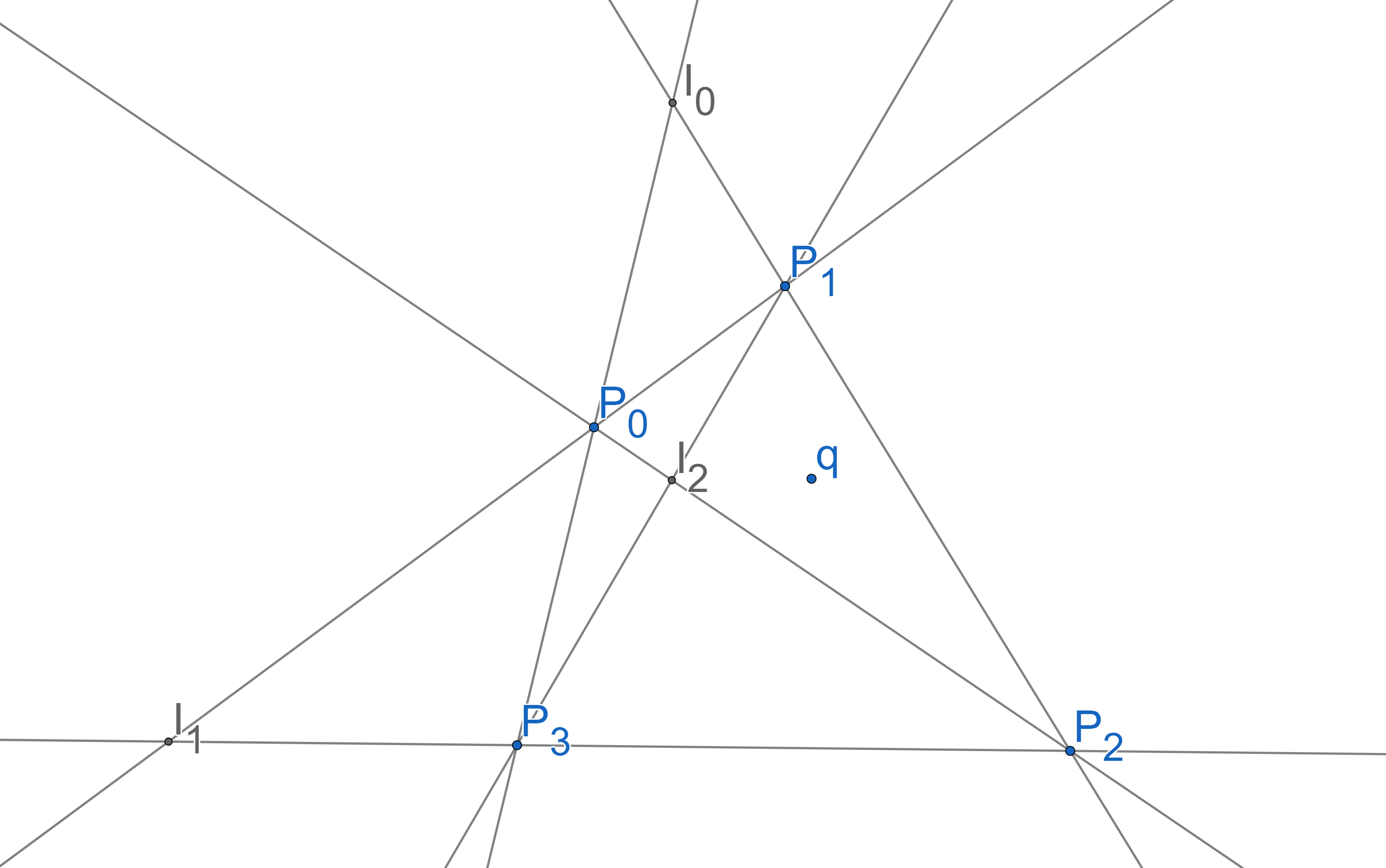
It is worth noting that the derivative of the equation (3) exists if $q$ is not on any of the hyperplanes in $H_{P}$ ($g_{i,q}\neq 0$). Now to find the HDD median with the minimum HDD measure, we should compute the derivative with respect to $q$ and see where it will be equal to $0$. For any query point $q$ inside a region bounded by some $H_{P}$ hyperplanes and not on any $H_{P}$ hyperplanes (Figure 1) we have

$$\begin{split}\frac{d}{dq}D_{P}(q)&=\frac{d}{dq}\sum_{h_{i}\in H_{P}}g_{i,q}\frac{{w_{i}}.q+{b_{i}}}{\|{w_{i}}\|}\\ &=\sum_{h_{i}\in H_{P}}g_{i,q}\frac{{w_{i}}}{\|{w_{i}}\|}\end{split}$$

(4)

Equation (4) above cannot be equal to $0$ in general since there are no variables (4). This means the assumption we made about the query point not being on the hyperplanes in $H_{P}$ was incorrect. Therefore, we can say the median is surely on one of the hyperplanes. If $q$ is on $h_{j}$, ${w_{j}}.q+{b_{j}}$ will be equal to $0$. Therefore, we can say

	$\displaystyle\frac{d}{dq}D_{P}(q)$	$\displaystyle=\frac{d}{dq}\sum_{h_{i}\in H_{P}-\{h_{j}\}}g_{i,q}\frac{{w_{i}}.q+{b_{i}}}{\|{w_{i}}\|}$
		$\displaystyle=\sum_{h_{i}\in H_{P}-\{h_{j}\}}g_{i,q}\frac{{w_{i}}}{\|{w_{i}}\|}.$		(5)

Using the same logic we can conclude that the median point should be on another hyperplane in addition to $h_{j}$. We can repeat these steps $d$ times and after that, it will be proved that the median should be on the intersection point of $d$ hyperplane (that will be a single point), thus the median will be on one of the intersection points.

Let $D^{\prime}_{p_{i}}(q)$ be the sum of the distances to all the hyperplanes in $H_{P}$ passing through the point $p_{i}$. The minimum of this convex function is always on the point $p_{i}$ where the HDD is equal to $0$. On the other hand, since each hyperplane includes $d$ input points from $P$, we have $D_{P}(q)=d\sum_{p_{i}\in P}{D^{\prime}_{p_{i}}(q)}$.
Now consider a point $q_{o}$ outside of the convex hull. by computing the gradient of $D_{P}(q_{o})$, we will show that by moving $q_{o}$ closer to the convex hull, the HDD gets smaller. Using the equation above we have $-\nabla H_{P}(q_{o})=-d\sum_{p_{i}\in P}\nabla{D^{\prime}_{p_{i}}(q_{o})}$. Since the minimum of the function $D^{\prime}_{p_{i}}(q)$ is on $p_{i}$, $-\nabla D^{\prime}_{p_{i}}(q)$ is a vector pointing to $p_{i}$ for $p_{i}\in P$. Therefore we can conclude that for every point $q_{o}$ outside of the convex hull, $-\nabla H_{P}(q_{o})$ points to the convex hull that means by moving toward that direction, the HDD decreases. Therefore the HDD median is always in the convex hull of $P$.

Let $p_{M}$ be the median of the $P$ s.t. $P$ is symmetric. If $p_{M}$ is not on the center of symmetry, consider ${p^{\prime}}_{M}$, the reflection of $p_{M}$ across the center of symmetry. Because of the symmetry, it is trivial that the HDD measure of both points is equal. Since the median point has the minimum depth measure among the other points and the depth measure function is convex, all the points on the line segment $p_{m}{p^{\prime}}_{M}$ should have a depth measure equal to the median. Therefore, the median is always at the center of symmetry.

As we move the query point $q$ to infinity, it is straightforward that there exists a hyperplane $h_{i}\in H_{P}$ that gets further from $q$. Since we can move $q$ arbitrarily far from $h_{i}$, and the distance from $q$ to the remaining hyperplanes in $H_{P}$ is non-negative, therefore HDD vanishes at infinity.

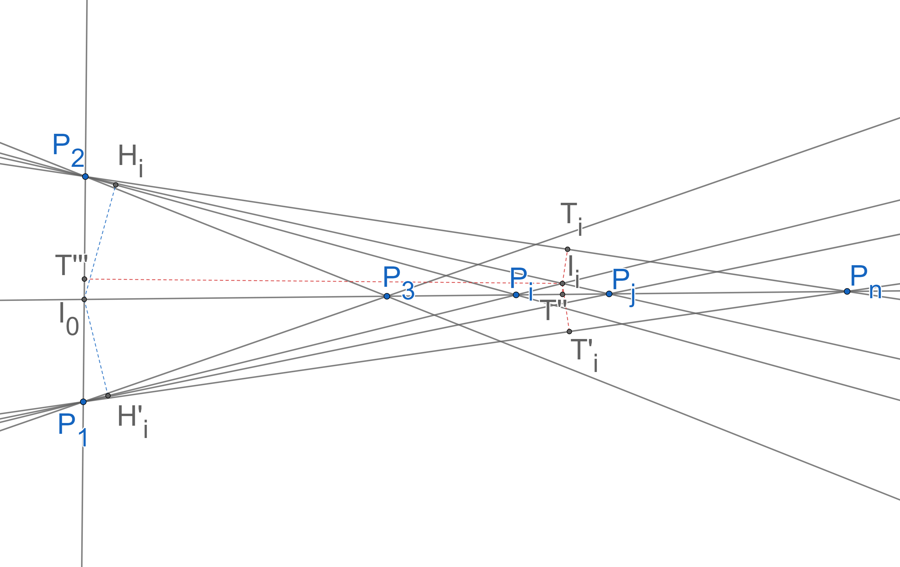
We will prove this fact using a counter-example in a 2-dimensional space (Figure 2). We can move the HDD median by changing the location of 2 points which means the HDD is not robust. The median is always on one of the intersection points and we can place the points in a way that $I_{0}$ is always the median (Figure 2). We will compute the depth measures for the points $I_{0}$ (5) and $I_{i}$ (7), where $I_{i}$ is an arbitrary intersection point except $I_{0}$.

	$\displaystyle D_{P}(I_{0})$	$\displaystyle=\sum_{i\in[3,n]}{d_{l_{P_{1}P_{i}}}(I_{0})}+\sum_{i\in[3,n]}{d_{l_{P_{2}P_{i}}}(I_{0})}$		(6)
	$\displaystyle D_{P}(I_{i})$	$\displaystyle=\sum_{i\in[3,n]}{d_{l_{P_{1}P_{i}}}(I_{i})}+\sum_{i\in[3,n]}{d_{l_{P_{2}P_{i}}}(I_{i})}$
		$\displaystyle+\binom{n-2}{2}d_{l_{P_{3}P_{n}}}(I_{i})+d_{l_{P_{1}P_{2}}}(I_{i})$		(7)

Regardless of the $I_{0}$ position, we know that $I_{0}H_{i}<I_{0}P_{2}$ and $I_{0}H^{\prime}_{i}<I_{0}P_{1}$. Therefore, we have (Equation (6)):

$$D_{P}(I_{0})<(n-2)I_{0}P_{2}+(n-2)I_{0}P_{1}=(n-2)P_{1}P_{2}$$

(8)

On the other hand, using Equation (7) we have:

$$D_{P}(I_{i})>d_{l_{P_{1}P_{2}}}(I_{i})$$

(9)

Now by moving the points $P_{1}$ and $P_{2}$ far enough, let $d_{l_{P_{1}P_{2}}}(I_{i})=(n-2)P_{1}P_{2}+m$, where $m$ is a positive number. Therefore, we have (inequality 9):

$$D_{P}(I_{i})>(n-2)P_{1}P_{2}+m$$

(10)

Combining the inequality 8 and 10 we have $D_{P}(I_{i})>D_{P}(I_{0})$.

Consequently, $I_{0}$ is the median. By increasing $m$, the median $I_{0}$ gets as far as we want. This means by moving $P_{1}$ and $P_{2}$, we can move the median point as much as we want.

Choose any $k>0$ and let $n=\max\{1,\lceil 1/k\rceil+1\}$. Let $P$ be a set of $n$ points in $\mathbb{R}$ and let $q\in\mathbb{R}$ lie to the left of $P$. By moving all points of $P$ one unit to the right ($\epsilon=1$), the hyperplane depth of $q$ relative to $P$ increases by a factor of $n$, regardless of $k$. Thus HDD is not $k$-stable.

We will prove this theorem using a counter-example. Consider the set of points $P=\{p_{0}(0,0),p_{1}(4,0),p_{2}(2,1)\}$. Using Theorem 3.5 we can show that the median is on point $p_{2}(2,1)$. Now consider the set $P^{\prime}=\{p^{\prime}_{0}(0,0),p^{\prime}_{1}(4,0),p^{\prime}_{2}(2,5)\}$ that is $P$ under the non-uniform affine transformation matrix $\begin{bmatrix}1&0\\ 0&5\end{bmatrix}$. Using theorem 3.5 and 3.9 It can be shown that the median is on the line $p^{\prime}_{0}p^{\prime}_{1}$ now. This means that the HDD median is not equivariant under affine transformation.

For any rotation, reflection, or translation transformation $f$, the distance from the query point $q$ to any hyperplane $h_{i}$ remains unchanged. That is, for any point $q$ and any hyperplane $h_{i}$, $\operatorname{dist}(q,h_{i})=\operatorname{dist}(f(q),f(h_{i}))$.

For any uniform scaling transformation $f$ with a scaling factor of $k$, distances between each pair of points will be multiplied by $k$ after the transformation. Therefore it is easy to show that, for any query point $q$, the HDD will be multiplied by $k$ after uniform transformation. Therefore, the median is equivariant under the uniform scaling transformation.

Let $l_{a}$ be an arbitrary line among the lines in $H_{P}$ (see Figure 3). There are $n\choose 2$ lines in $H_{P}$ and, consequently, $O(n^{2})$ points of intersection between $l_{a}$ and lines in $H_{P}$. Using an analogous argument as in the proof of Theorem 3.5, the point with minimum HDD on $l_{a}$ lies at an intersection of $l_{a}$ and a line in $H_{P}$. Therefore, using the same algorithm described in Section 4.2, we can find the point $i_{\min}$ on $l_{a}$ with minimum HDD in $O(n^{2}\log n)$ time; let $h_{\min}$ denote the line in $H_{P}$ such that $i_{\min}=h_{\min}\cap l_{a}$. Next, we find the closest points of intersection in $H_{P}$ to $i_{\min}$ on the line $h_{\min}$ in each direction, say $I_{u}$ and $I_{d}$. We compute the HDD for all the three points $i_{\min}$, $I_{d}$, and $I_{u}$. Since $i_{\min}$ has minimum HDD on the line $l_{a}$, if $D_{P}(i_{\min})<\min\{D_{P}(I_{u}),D_{P}(I_{d})\}$, then $i_{\min}$ is the HDD median (by Theorem 3.3). By Theorem 3.3 again, $D_{P}(i_{\min})<D_{P}(I_{u})$ or $D_{P}(i_{\min})<D_{P}(I_{d})$. Furthermore, $D_{P}(i_{\min})>D_{P}(I_{u})$ or $D_{P}(i_{\min})>D_{P}(I_{d})$. Without loss of generality, suppose $D_{P}(I_{d})<D_{P}(i_{\min})<D_{P}(I_{u})$. We claim that all points in the half-plane bounded by $h_{\min}$ that contains $I_{u}$ have HDD that exceeds $D_{P}(i_{\min})$; we prove this by contradiction. Suppose there exists a point $A$ in this half-plane such that $D_{P}(A)<D_{P}(i_{\min})$. Let $B$ be the intersection point of the line $l_{a}$ and the line segment $\overline{AI_{d}}$. Since $i_{\min}$ has minimum HDD on the line $l_{a}$, therefore, $D_{P}(i_{\min})<D_{P}(B)$. Furthermore, $D_{P}(A)<D_{P}(B)$. On the other hand, we assumed $D_{P}(I_{d})<D_{P}(i_{\min})<D_{P}(I_{u})$ and we know $D_{P}(i_{\min})<D_{P}(B)$. Consequently, $D_{P}(I_{d})<D_{P}(B)$. Combining the two resulting inequalities above, we have $D_{P}(A)<D_{P}(B)$ and $D_{P}(I_{d})<D_{P}(B)$, which is impossible since the three points are on the same line and the HDD function is convex. Therefore, no such point $A$ can exist.

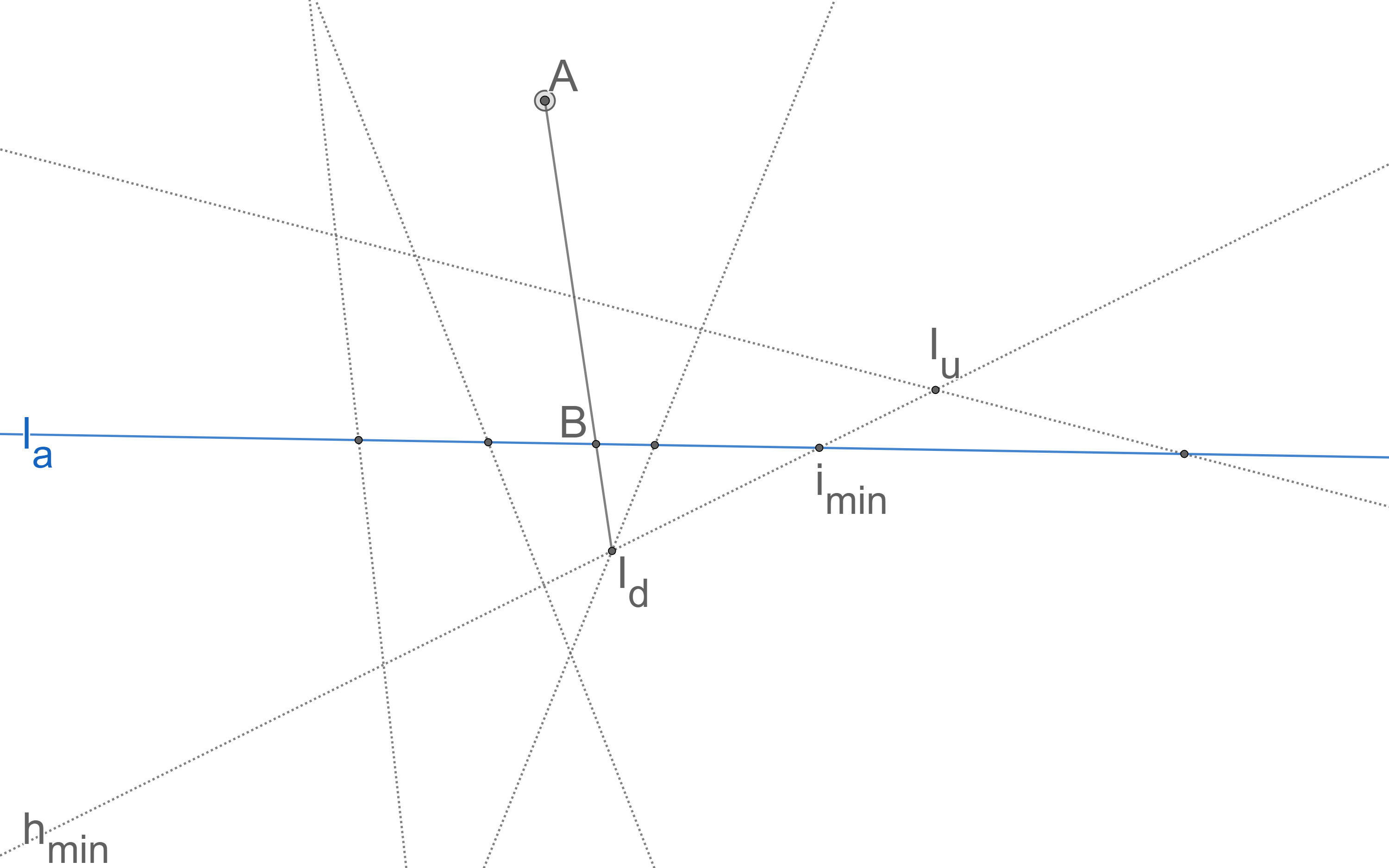
Therefore, no point of intersection in $H_{P}$ in this half-plane can be an HDD median of $P$; in $O(n^{2}\log n+3n^{2})\subseteq O(n^{2}\log n)$ time we can remove these points from consideration in our search for a median.

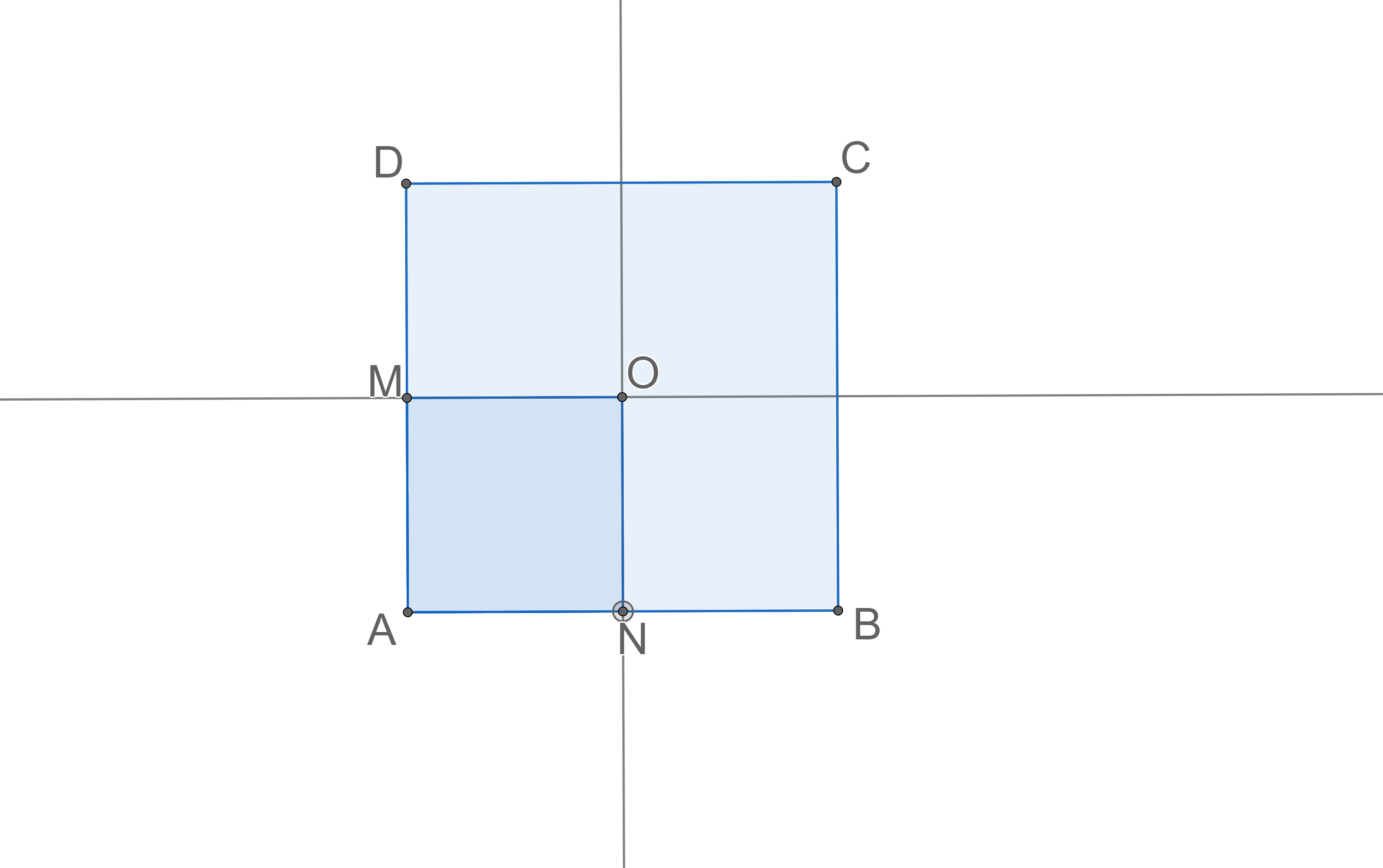
Now we will use this property to approximate the median point. Firstly, we will find the diameter $a$ of the input points in $O(n)$ time and consider an $a\times a$ square that contains $P$ (see Figure 4). By Theorem 3.7, we know that the median lies inside this square. At each step, we draw the two lines $ON$ and $OM$ that partition the square into four similar smaller squares, each with dimensions $\frac{a}{2}\times\frac{a}{2}$, and we apply the above algorithm to eliminate two half-planes in $O(n^{d}\log n)$ time. After $m$ steps we have a square of dimensions $\frac{a}{2^{m}}\times\frac{a}{2^{m}}$ and we return its center as an approximation of the HDD median. Since the HDD median is a point inside this square, the error is at most $\frac{a\sqrt{2}}{2^{m+1}}$. The total time complexity of the algorithm is $O(mn^{2}\log n)$.

References

- [1] C. Bajaj. The algebraic degree of geometric optimization problems. Discrete and Computational Geometry, 3:177–191, 1988.
- [2] V. Barnett. The ordering of multivariate data. Journal of the Royal Statistical Society: Series A (General), 139(3):318–344, 1976.
- [3] B. Chazelle and J. Friedman. Point location among hyperplanes and unidirectional ray-shooting. Computational Geometry, 4(2):53–62, 1994.
- [4] R. Durier and C. Michelot. Geometrical properties of the Fermat-Weber problem. European Journal of Operational Research, 20(3):332–343, 1985.
- [5] S. Durocher and D. Kirkpatrick. The projection median of a set of points. Computational Geometry: Theory and Applications, 42(5):364–375, 2009.
- [6] S. Durocher, A. Leblanc, and M. Skala. The projection median as a weighted average. Journal of Computational Geometry, 8(1):78–104, 2017.
- [7] R. Z. Farahani, M. SteadieSeifi, and N. Asgari. Multiple criteria facility location problems: A survey. Applied mathematical modelling, 34(7):1689–1709, 2010.
- [8] R. Y. Liu. On a notion of data depth based on random simplices. The Annals of Statistics, pages 405–414, 1990.
- [9] P. C. Mahalanobis. On the generalized distance in statistics. Sankhyā: The Indian Journal of Statistics, Series A (2008-), 80:S1–S7, 2018.
- [10] A. T. Murray and V. Estivill-Castro. Cluster discovery techniques for exploratory spatial data analysis. International journal of geographical information science, 12(5):431–443, 1998.
- [11] H. Oja. Descriptive statistics for multivariate distributions. Statistics & Probability Letters, 1(6):327–332, 1983.
- [12] J. Tukey. Mathematics and the picturing of data. In Proc. Int. Cong. Math., pages 523–531, 1957.
- [13] Y. Vardi and C.-H. Zhang. The multivariate -median and associated data depth. Proceedings of the National Academy of Sciences, 97(4):1423–1426, 2000.
- [14] Y. Zuo and R. Serfling. General notions of statistical depth function. Annals of statistics, 28(2):461–482, 2000.