Hyperplane families creating envelopes
Abstract.
A simple geometric mechanism: “the locus of intersections of perpendicular bisectors and normal lines”, often arises in many guises in Nonlinear Sciences. In this paper, a new application of this simple geometric mechanism is given. Namely, we show that this mechanism gives answers to all four basic problems on envelopes created by hyperplane families (existence problem, representation problem, equivalence problem of definitions, uniqueness problem) at once.
Key words and phrases:
Hyperplane family, Frontal, Envelope, Creative, Creator, Mirror-image mapping, Anti-orthotomic, Orthotomic, Cahn-Hoffman vector formula.2010 Mathematics Subject Classification:
57R45, 58C251. Introduction
Throughout this paper, let be a positive integer. Moreover, all manifolds, functions and mappings are of class unless otherwise stated.
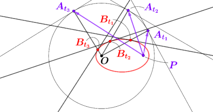
A simple geometric mechanism: “the locus of intersections of perpendicular bisectors and normal lines”, often arises in many guises in Physical Sciences. For example, as Richard Feynman elegantly explained in [9], the orbit of a planet around the sun can be understood as a consequence of this mechanism under the assumption of the inverse-square law (see Figure 2 where the circle is the hodograph of the velocity vectors of a planet , that is to say, the circle is a curve drawn by the end points of the vectors that are parallel to the velocity vectors and start at a fixed point . The orbit of the planet is similar to the locus of intersections of the perpendicular bisectors of velocity vectors and the normal lines to the circle at ). This is an example in Celestial Mechanics. In the same book [9], one can find that even the historical discovery of atomic nucleus due to Ernest Rutherford can be explained as a consequence of this simple geometric mechanism (see Figure 2 where the center of circle is an atomic nucleus. The orbit of an particle is the locus of intersections of the perpendicular bisectors of the segment and the normal lines to the circle at ). This is an example in Nuclear Physics.
In Crystallography, one can find such the mechanism in the so-called Wulff construction for the equilibrium shape of a crystal. A brief explanation of the Wulff construction is as follows. Given an equilibrium crystal, take an arbitrary point inside the crystal and fix it. Georg Wulff discovered in [20] the so-called Gibbs-Wulff theorem which asserts that the length from the fixed point to the foot of the perpendicular to the tangent space to the face of the crystal is proportional to its surface energy density of the face. Let be the surface energy density function of the equilibrium crystal. The graph of with respect to the polar coordinates about the point defines the mapping . The mapping is often called the polar plot of or the -plot or the Wulff plot. Set and suppose that the image has the well-defined normal vectors at any point . Then, by the Gibbs-Wulff theorem, the accurate shape of the crystal surface is proportional to the shape obtained by our simple geometric mechanism: “the locus of the intersection of the perpendicular bisector of the vector and the normal line to at ”. This is the Wulff construction and the constructed shape is called the Wulff shape. Notice that in general is a continuous mapping and thus from the viewpoint of rigorous mathematics, the Wulff construction is not a well-defined construction method in general. Nevertheless, Hoffman and Cahn showed in [11] that if is differentiable, then the image has a well-defined normal vector at each point and the set is exactly the shape obtained by our simple geometric mechanism for the point and the surface . The Wulff construction and the Cahn-Hoffman formula in the plane is depicted in Figure 3. For details on the Wulff construction and Wulff shapes, see for instance [8, 10].
Moreover, it is a surprising fact that our simple geometric mechanism: “the locus of intersections of perpendicular bisectors and normal lines”can be applied even to Seismic Survey (see 7.14 (9) of [6]).
In Mathematics, our simple geometric mechanism: “the locus of intersections of perpendicular bisectors and normal lines”is called the anti-orthotomic of a mapping having a well-defined normal vector to its image at each point (for details on anti-orthotomics, see 7.14 of [6]. See also [15] where anti-orthotomics are generalized to frontals and [16] where more elementary explanation on anti-orthotomics can be found). In Mathematics as well, there are examples where anti-orthotomics are effectively applied (see [6]).
In order to understand better the powerfulness
of the simple geometric mechanism,
we would like to have more striking
examples in Mathematics where anti-orthotomics are
effectively applied. Namely, we want to seek
mathematical problems
which can be geometrically solved by our simple geometric mechanism
though it seems difficult to solve them by other methods.
This is the primitive motivation of this paper.
In this paper, we show that the existence and uniqueness problem of envelopes
for a given hyperplane family is one of such problems.
Namely, we give a necessary and sufficient condition
(see Definition 2) for a given hyperplane family
to create an envelope. And then, we give a necessary and sufficient
condition for the uniqueness of created envelopes
if the given hyperplane family creates an envelope.
It seems difficult to prove that the condition
given in Definition 2 is actually a sufficient condition to create
envelopes by other methods.
In order to apply our simple geometric mechanism,
we need some geometric objects
to which the normal line can be reasonably well-defined at each point.
Hyperplane families themselves are
far from the reasonable geometric objects for our purpose.
The reasonable geometric objects are frontals
(the definition of frontal is given in the next paragraph).
In order to obtain a frontal from a given hyperplane family,
the mirror-image mapping will be locally introduced.
Then, it turns out that if the given hyperplane family is creative
(see Definition 2 below),
then the mirror-image mapping is actually a frontal such that the normal
line at each point intersects the corresponding hyperplane.
Thus, we can apply the anti-orthotomic method developed
in [15] to obtain Theorem 1
and Theorem 2.
The existence and uniqueness
problem of envelopes for a given hyperplane family
can be easily interpreted as the existence
and uniqueness problem of solutions for a
certain type of system of first order differential equations
with one constraint condition.
In the author’s opinion, one of the most attractive features
of our simple geometric mechanism is
that it can make all solutions and their precise
expressions clear in one shot by geometry
without the need to solve the corresponding system
of differential equations with
one constraint condition.
Let be the -dimensional unit sphere in the -dimensional vector space . Given a point of and an -dimensional unit vector , the hyperplane relative to and is naturally defined as follows, where the dot in the center stands for the standard scalar product of two vectors and in the vector space .
Let be an -dimensional manifold without boundary. Given two mappings and , the hyperplane family relative to and is naturally defined as follows.
A mapping is called a frontal if there exists a mapping such that for any and any , where two vector spaces and are identified. By definition, it is natural to call a Gauss mapping of the frontal . The notion of frontal has been recently investigated (for instance, see [13]). In this paper, as the definition of envelope created by a hyperplane family, the following is adopted.
Definition 1.
Let be a hyperplane family. A mapping is called an envelope created by if the following two conditions are satisfied.
-
(a)
for any .
-
(b)
for any and any .
In other words, an envelope created by is a mapping giving a solution of the following system of first order differential equations with one constraint condition, where is an arbitrary coordinate neighborhood of such that .
By definition, any envelope created by a hyperplane family must be a frontal with Gauss mapping . For details on envelopes created by families of plane regular curves, refer to [6]. In Chapter 5 of [6], several definitions for envelope are given. For a hyperplane family , Definition 1 is a generalization of their definition from a viewpoint of parametrization ( envelope is a variety tangent to all lines of the given line family. Thus, in the case of plane, an envelope defined by Definition 1 is the same notion of envelope. For details on the definition , see 5.12 of [6]). The following definition, which may be regarded as a higher dimensional generalization of from a viewpoint of parametrization ( envelope is the set of the limits of intersections with nearby members of the given line family. For details on the definition , see 5.8 of [6] and for the relation between Definition 2 in the plane case and , see Subsection 2.3), is the key notion for this paper.
Definition 2.
Let be an -dimensional manifold without boundary and let , be mappings. Let be the function defined by . Let be the cotangent bundle of . A hyperplane family is said to be creative if there exists a mapping with the form such that for any the equality holds as germs of -form at .
Namely, is creative if there exists a -form along such that for any by using of a coordinate neighborhood of at and a normal coordinate neighborhood of at , the -form germ at is expressed as follows.
where a normal coordinate neighborhood is a local coordinate neighborhood at obtained by the inverse mappping of the exponential mapping at , inherits its metric from the ambient space and is the Levi-Civita translation. Notice that our objective manifold is the unit sphere with metric inherited from . Therefore, the Levi-Civita translation is the restriction of the rotation satisfying to the tangent space . In particular, in the case , a normal coordinate at is nothing but the radian (or, its negative) between two unit vectors and and the Levi-Civita translation is just the restriction of the plane rotation through to the tangent space .
Remark 1.1.
-
(1)
It is reasonable to say that is totally differentiable with respect to if is creative.
- (2)
-
(3)
Definition 2 may be interpreted as follows. Let be a canonical contact -form on , namely at any the -form germ is expressed as , where is a normal coordinate system at and is a canonical coordinate system of at . Then, a hyperplane family is creative if there exists a mapping with the form such that , where are some functions.
Notice that in Legendrian Singularity Theory, at any point , the map-germ is assumed to be immersive and it is called a Legendrian immersion; and for Legendrian immersion , the mapping is called a wavefront or front (for details on Legendrian Singularity Theory and fronts, see for instance [1, 2, 17]). On the other hand, in Definition 2, is not assumed to be immersive in general and the mapping is called a Legendrian mapping (for details on Legendrian mappings, see for instance [12, 13, 18]). Thus, in Definition 2, in general, the set-germ may be singular at some point (for example, see Example 4.1(4)).
-
(4)
Notice that the -form along in Definition 2 is not necessarily the pullback of a -form over by (for example, see Example 4.1(3), (4)) and the “creativeness” does not depend on the particular choice of and depends only on the hyperplane family . In the case that and is the identity mapping, for any the hyperplane family is always creative by the following equality.
More generally, if may be expressed as the composition of and a certain function over an open set , then the hyperplane family is creative. However, there are examples showing that there does not exist a function such that although is creative (for example, see Example 4.1(3), (4)). Moreover, there are many examples such that is not creative. For instance, for any constant mapping , the line family is not creative where is defined by . And, it is clear in this case that does not create an envelope in the sense of Definition 1. However, it is easily seen that
where . Thus, for this example, the envelope defined by Definition 1 is different from the envelope in the sense of classical definition (see 5.3 of [6]), For more examples on creative/non-creative hyperplane families and on comparison of Definition 2 with the classical envelope , see Section 4. Therefore, it seems that the current situation on both the definitions of envelope and the relation of the creative condition (Defnition 2) with an envelope seems to be wrapped in mystery.
By definition, any frontal with Gauss mapping is an envelope created by . Therefore, the notion of envelope created by a hyperplane family is the same as the notion of frontal. Moreover, it is clear that for any mapping , a constant mapping is an envelope created by . On the other hand, for a constant mapping , if the line family does not create an envelope then must be not constant. From these elementary observations, it is natural to ask to obtain a necessary and sufficient condition for a given hyperplane family to create an envelope in terms of and . Moreover, it is also desirable to solve the following two incidentally. “Suppose that a given hyperplane family creates an envelope . Then, obtain a representation formula of .” “Suppose that . Then, find the precise relation between envelope and envelope.” In this paper, as an application of our simple geometric mechanism, all of these problems are solved as follows.
Theorem 1.
Let be an -dimensional manifold without boundary and let , be mappings. Then, the following three hold.
-
(1)
The hyperplane family creates an envelope if and only if it is creative.
-
(2)
Suppose that the hyperplane family creates an envelope . Then, for any , under the canonical identifications , the -dimensional vector is represented as follows.
where the -dimensional vector is identified with the corresponding -dimensional cotangent vector under these identifications.
-
(3)
Suppose that . Then, the line family creates an envelope (-envelope) if and only if it creates an envelope. Moreover, these two envelopes are exactly the same.
By Theorem 1, it is natural to call the creator for an envelope created by . Recall that envelope (resp., envelope) is the set of the limit of intersections with nearby lines (resp., a parametrization tangent to all members of the given family). Thus, even in the case of plane, envelope is exactly the same as the envelope in Definition 1.
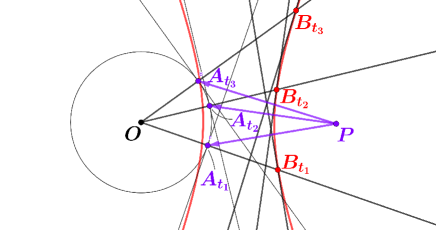
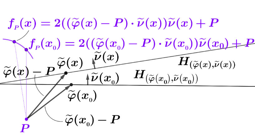
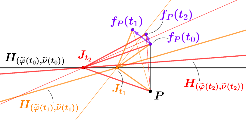
The key idea for the proof of Theorem 1 is to regard the given hyperplane family as a moving mirror parametrized by . Then, for any parameter , by taking a point outside the mirror , the mirror-image
of by the mirror must have the same information as the mirror since the mirror is reconstructed as the perpendicular bisectors of the segment , where is a point in a sufficiently small neighborhood of .
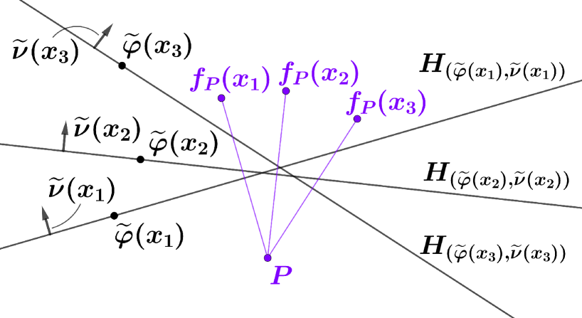
Hence, investigation of the given hyperplane family may be replaced with analyzing the associated mirror-image mapping (see Figure 4). This suggests applicability of results in [15] to the problem of this paper.
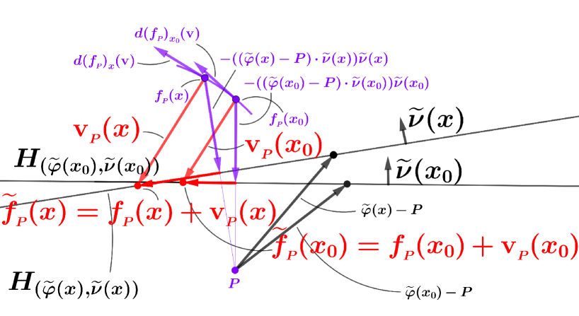
A sketch of the proof of Theorem 1 (1) may be given as follows. Suppose that the hyperplane family is creative. Then, by definition, there exists a mapping having the form such that the equality holds as germs of -form at . Then, by investigating the Jacobian matrix of the mirror-image mapping at directly, it turns out that for any the non-zero vector
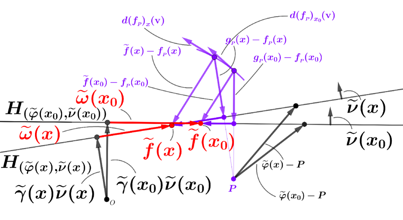
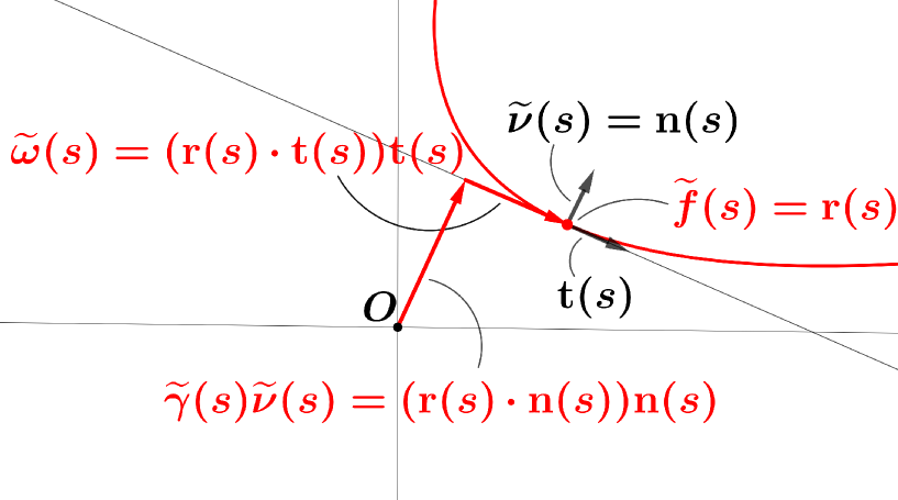
is perpendicular to the vector for any , where , and are identified and . Thus, is a frontal. From the construction, the mapping must be exactly the same as the mapping given in Theorem 1 of [15]. Therefore, by Theorem 1 of [15] asserting that satisfies both conditions (a), (b) of Definition 1, is an envelope created by the hyperplane family . The mapping is called the anti-orthotomic of relative to . Calculation shows
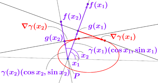
Thus, unlike , the location does not depend on the particular choice of . In other words, in order to discover the formula , the role of is merely an auxiliary point just like an auxiliary line in elementary geometry (see Figure 5).
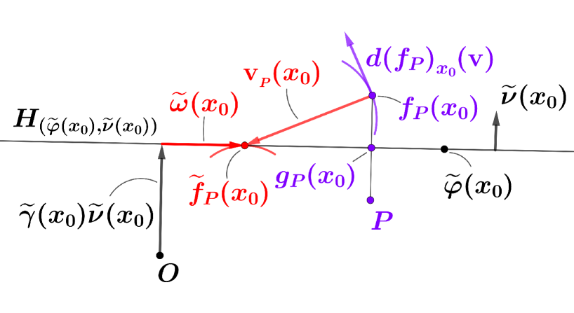
Since is an arbitrary point of , the hyperplane family creates an envelope .
Conversely, suppose that the given hyperplane family creates an envelope . Then, the mirror-image mapping (resp., the mapping defined by ) is called the orthotomic (resp., pedal) of relative to the point . It is known that both the orthotomic and the pedal are frontals (see Proposition 1 and Corollary 1 of [15]). We prefer to investigate the orthotomic rather than the pedal because its Gauss mapping has characteristic properties: and for any , and thus we can take a bird’s eye view of . Set and for any . Then, under the identification of and , having the form is a well-defined mapping . By investigating the Jacobian matrix of the mirror image mapping at directly again, it turns out that is actually the creator for the envelope . Since the vector does not depend on the particular choice of and the point is an arbitrary point of , is creative.
Theorem 1 (2) is a direct by-product of the proof of Theorem 1 (1) (see Figure 5). Theorem 1 (3) seems to be not a direct by-product of the proof of Theorem 1 (1) although it can be proved relatively easily by using the above argument (see Subsection 2.3).
When and is the identity mapping, it is easily seen . Therefore, in the case that and is the identity mapping, Theorem 1 (2) has been known as the Cahn-Hoffman vector formula ([11]). Theorem 1 (2) is a comprehensive generalization of their formula. Any Wulff shape is clearly a convex body and conversely it is known that any convex body can be constructed by the Wulff construction (for instance, see [19]). There are many Wulff shapes such that the surface energy density functions are not differentiable (convex polytopes are typical examples). Thus, for studing Wulff shapes having non-smooth surface energy functions, it is very significant to answer the following two problems: “(a) Generalize Cahn-Hoffman vector formula to the corresponding formula for any ”ȧnd “(b) Resolution of singularities of the boundary of a convex body having non-smooth boundary by a frontal ”. By Theorem 1 (2), the problem (a) is completely solved. As for the problem (b), to the best of author’s knowledge, only the boundary of a square has been realized as a frontal so far (see [15]). Although there are apparently no published proofs at present, it is a comparatively straightforward generalization of this result to show that the boundary of a convex polygon is realized as a frontal . However, even in the plane case, the problem (b) for the boundary of a convex body in general seems to be wrapped in mystery.
Moreover, Theorem 1 (2) might be useful even for the study of force problems in higher dimensional vector spaces. In [4], Petr Blaschke discovered that pedal coordinates are more suitable settings to study force problems in . Readers who want to confirm their usefulness are recommeded to refer to [4] (see also 7.24 (6) of [6] though this is not a force problem but a very suitable problem for understanding how useful pedal coordinates are). Theorem 1 (2) may be regarded as a higher dimensional generalization of pedal coordinates. Hence, it is expected that Theorem 1 (2) is a very suitable expression to study force problems etc. in all finite-dimensional vector spaces over . Example 4.2 (2) might be regarded as examples in which higher dimensional version of pedal coordinates are effectively used.
As an application of Theorem 1, a characterization for a hyperplane family to create a unique envelope is given as follows.
Theorem 2.
Let , be mappings. Then, the hyperplane family creates a unique envelope if and only if it is creative and the set consisting of regular points of is dense in .
Under the assumption that in Remark 1.1 (2) is immersive and some conditions are satisfied, a unique existence result of envelopes for hyperplane families has been obtained in [7]. Since their assumptions clearly imply that the creative condition defined in Definition 2 is satisfied and the set consisting of regular points of is dense, their result follows from Theorem 1 and Theorem 2.
Notice that non-unique existence cases, too, are intriguing cases since Theorem 1 may be effectively applied even in such cases (see Example 4.2 (1), (2)).
This paper is organized as follows. Theorem 1 and Theorem 2 are proved in Section 2 and Section 3 respectively. In Section 4, examples are given. Section 5 is an appendix where an alternative proof of Theorem 1 except for Theorem 1 (3) is given. The alternative proof is a proof by a gauge theoretic approach. In order to avoid unnecessary complication, the alternative proof is given only in the case . The author has no idea on how to prove Theorem 1 (3) by using the alternative proof.
2. Proof of Theorem 1
2.1. Proof of Theorem 1 (1)
2.1.1. Proof of “if” part
Let be an arbitrary point of . Take one point of and fix it. It follows . Let be the set of points satisfying
Then, it is clear that is an open neighborhood of and the mirror image of the fixed point by the mirror is given by
for any .
Since the hyperplane family is assumed to be creative, there exists a mapping with the form such that for any the following equality holds as -form germs at .
Let be a normal coordinate neighborhood of at . Set . Consider the mirror-image mapping defined by
for any . In order to show that is a frontal, it is sufficient to construct a Gauss mapping with respect to . By using the mapping , a Gauss mapping for is constructed as follows. For any set . Let be the Levi-Civita translation. For any , set . Then notice that for any , under the identification of and ,
is an orthonormal basis of the tangent vector space .
Lemma 2.1.
For any , the following equality holds.
By Lemma 2.1, under the identification of and , it follows
for any . Set
for any where and are identified and and are identified. By (), is not the zero vector. Moreover, the following holds.
Lemma 2.2.
For any , is perpendicular to .
Proof of Lemma 2.2. Calculation of the product of the vector and the Jacobian matrix of at (denoted by ) is carried out as follows, where and are identified and and are identified.
We may consider that the point is an arbitrary point of . Thus we have the following.
Lemma 2.3.
The mapping is a frontal with Gauss mapping such that , where .
By Lemma 2.3, the hyperplane and the line must intersect only at one point for any . Define the mapping by
Then, from the construction, must have the following form (see p.7 of [15]).
By Theorem 1 of [15] (more precisely, by 3.1 in p.9 of [15]) and Lemma 2.3, we have the following.
Lemma 2.4.
The mapping is a frontal with Gauss mapping . In other words, is an envelope created by the hyperplane family .
On the other hand, it is easily seen that (see Figure 7). Thus, the vector must belong to . From the construction and by using the equality we have the following.
This proves the following lemma.
Lemma 2.5.
The following equality holds.
2.1.2. Proof of “only if” part
Suppose that the hyperplane family creates an envelope . Then, by definition, is a frontal such that the inclusion holds for any . Let be the mapping defined by (see Figure 8).
It is sufficient to show that under some identifications, is actually a creator for the envelope .
It is easily seen that for any . Thus, under the identification of and , we have
Lemma 2.6.
For any , holds.
Let be the mapping defined by . Let be an arbitrary point of and let be a point of . Again, we consider the mirror-image mapping defined by
where . The mapping is exactly the orthotomic of relative to the point . Thus, by Proposition 1 of [15] (more precisely, by 2.1 in pp. 7–8 of [15]) , is a frontal and the mapping define by
is its Gauss mapping. In particular, we have the following.
Lemma 2.7.
For any and any , the following holds.
For any , set
Then, since is the mirror-image of with respect to the mirror , the following clearly holds.
Lemma 2.8.
The vector is perpendicular to the vector for any .
In order to decompose the vector reasonably, the open neighborhood of is reduced as follows. Let be a normal coordinate neighborhood of at . Set again . Notice that is an orthonormal basis of the cotangent space .
Lemma 2.9.
The equality
holds where three vector spaces , and are identified.
By Lemma 2.9, the following holds.
Hence, by Lemma 2.1 and Lemma 2.7, the germ of -form at is calculated as follows, where , and is the Levi-Civita translation.
This calculation proves the following lemma.
Lemma 2.10.
The equality
holds as germs of -form at .
Since is an arbitrary point of , by Lemma 2.10, is actually the creator for the given envelope . This completes the proof of “only if” part.
2.2. Proof of Theorem 1 (2)
2.3. Proof of Theorem 1 (3)
Recall that the line family is said to create an envelope (denoted by in this subsection) if for any fixed and any near the limit exists. On the other hand, the line family is said to create an envelope (denoted by in this subsection) if it creates an envelope in the sense of Definition 1.
Let be a point of and let be a sequence conversing to . Since is assumed, we can assume that a point can be taken from the intersection such that exists. Denote the limit by . Then, we have the following.
This implies
Thus we have
This implies that there exists a real number such that the following identity holds where and stand for the -dimensional cotangent vectors in , namely the following identity is nothing but the identity of two real numbers.
It is not difficult to see that the function is of class . This means that the line family is creative. Therefore, by Theorem 1 (1), the line family creates an envelope. ∎
For the proof of this implication, it is used the notions and notations introduced in the proof of Theorem 1 (1). The assumption implies that is totally differentiable with respect to . Take an arbitrary point and fixed it. Since is totally differentiable with respect to at , for any near if the length of the vector is positive, then the horizontal vector of must be non-zero, where is a point taken outside the line and is a mirror-image mapping introduced in the proof of Theorem 1 (1). Denote the intersection of the perpendicular bisector of and the line by . Then, from the construction, it follows that the triangre is an isosceles triangle with legs and . This implies the following (see Figure 9).
Notice that is positive. Thus, we have
By Proposition 1 of [15] asserting that is a frontal with its Gauss mapping , it follows
where is the anti-orthotomic of relative to the point introduced in the proof of Theorem 1 (1). Since is an arbitrary point of , the given envelope must be an envelope by Theorem 1 (1). ∎
3. Proof of Theorem 2
Proof of “if” part. Since the hyperplane is creative, by Theorem 1, it creates an envelope. Let be envelopes created by .
Let be a regular point of . Then, there exists an open coordinate neighborhood such that and is a diffeomorphism. Then, the germ of -form at is
Let be the mapping with the form such that is the creator for . Then, by the above calculation, must have the following form.
Hence, by Theorem 1 (2), we have the following.
Lemma 3.1.
At a regular point of , the equality holds.
Let be a singular point of . Then, since we have assumed that the set of regular points of is dense, there exists a point-sequence such that is a regular point of for any and . Then, by Lemma 3.1, we have
Thus, we have the following.
Lemma 3.2.
Even at a singular point of , the equality holds.
Proof of “only if” part. Suppose that the hyperplane is creative and the set of regular points of is not dense in . Then, there exists an open set of such that any point is a singular point of . Then, there exist an integer and an open set such that and the rank of at is for any . Let be a point of . We may assume that is sufficiently small open neighborhood of . Then, by the rank theorem (for the rank theorem, see for example [5]), we have the following.
Lemma 3.3.
There exist functions such that the following three hold.
-
(1)
For any , if .
-
(2)
There exists an such that .
-
(3)
The following equality holds for any .
Since we have assumed that is creative, there exists a mapping with he form such that . By Lemma 3.3, the following holds.
Lemma 3.4.
For any function and any , the following equality holds as germs of -form at .
Therefore, by Theorem 1 (2), uncountably many distinct envelopes are created by the same hyperplane family .
4. Examples
Example 4.1 (Uniform spin of affine tangent lines).
-
(1)
Let be a non-constant function. Notice that is of class as stated at the top of Section 1. Let be the mapping defined by . Let be the constant mapping . For any fixed , let be the linear mapping representing the rotation through angle . Set and . Figure is depicted in Figure 10.
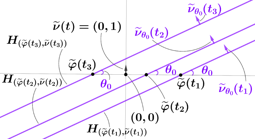
Figure 10. Figure for Example 4.1 (1). It follows and . Since is non-constant, there exists a regular point of , that is to say, there exists a such that . Therefore, by Theorem 1, the line family creates an envelope if and only if . Suppose that . In this case, by Theorem 2, uncountably many distinct envelope can be created by the given line family . Let be a function. Since and in this case, the -form along may be a creator for the line family. By Theorem 1 (2), the envelope has the following form.
where double sign should be read in the same order and , are identified (both are denoted by the same symbol ).
Set . Suppose that . In this case, the classical common definition of envelope relative to is as follows.
Therefore, in this case, if and only if is non-singular. Suppose that . Then,
Therefore, in this case, if and only if is surjective.
-
(2)
Let be the mapping given by . Set , where is the rotation defined in the above example. Then, since , it follows . Thus, by Theorem 1(1) and Theorem 2, for any the line family creates a unique envelope . For any , set . Since , by Theorem 1 (2), it follows
where the -form and the vector field are identified. Let be a function and set .
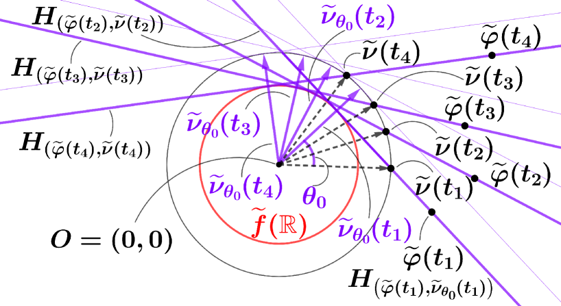
Figure 11. Figure for Example 4.1 (2). Then, it follows . Thus, as expected, the envelope created by the line family in this case is actually the circle with radius centered at the origin, where (see Figure 11).
-
(3)
Let be the mapping defined by . Set where is as above. Let be a function and set . Set . It is easily seen that is a singular point of if and only if . On the other hand, by calculation, we have and thus is a unique singular point of for any . Therefore, by Theorem 1, the hyperplane family does not create an envelope if .
Next, suppose that . Then, calculations show
where double sign should be read in the same order. Set . By Theorem 1 and Theorem 2, the hyperplane family creates a unique envelope with the desired form
where for each the cotangent vector and the vector in the vector space are identified (see Figure 12).
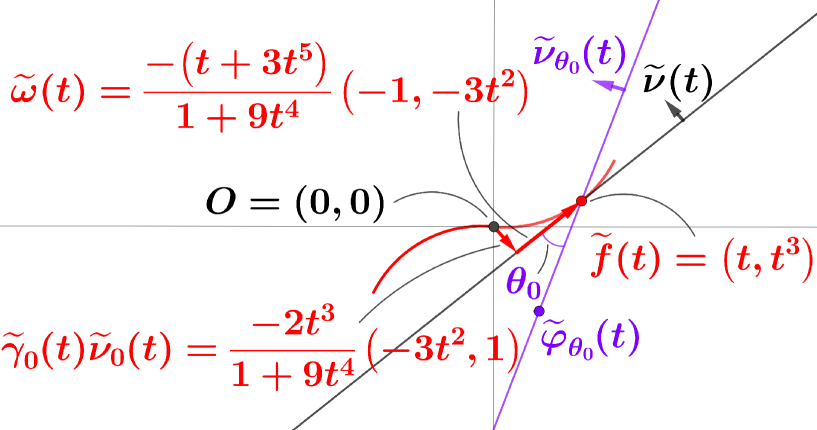
Figure 12. Figure for Example 4.1 (3) in the case . -
(4)
Let be the mapping defined by . Set where is as above. Let be a function and set . Set . By calculation, we have . Therefore, the hyperplane family is not creative if and it creates no envelope in this case by Theorem 1.
Next, suppose that . Then, calculation shows
where double sign should be read in the same order. Therefore, the hyperplane family is creative. Set . By Theorem 1 and Theorem 2, creates a unique envelope with the desired form
where for each the cotangent vector and the vector in the vector space are identified (see Figure 13).
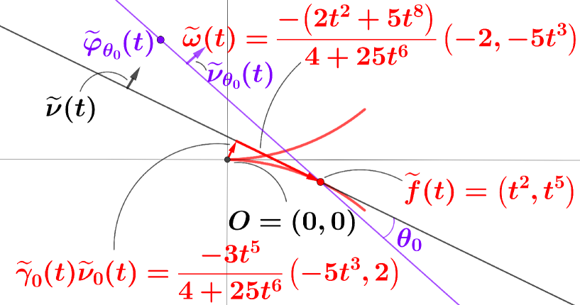
Figure 13. Figure for Example 4.1 (4) in the case .
Example 4.2 (Unit speed curves).
-
(1)
Let be a unit speed curve. As usual, set and is defined from t(s) by rotating anticlockwise through . The Serret-Frenet formulas for the plane curve is as follows.
Set and . Then, the line family is the affine tangent line family of the curve . In this case, the correspondence may be regarded as the Legendre transformation of the given curve . Set . Then,
where . Therefore, by Theorem 1, the line family creates an envelope.
Suppose that the set of regular points of is dense, that is to say, the set is dense. Then, by Theorem 2, the created envelopes are unique. By Theorem 1, the unique envelope is as follows (see Figure 14).
Notice that if there is a point such that , then the full discriminant of the line family is different from the unique desired envelope since the full discriminant includes the affine tangent line at . This is one of advantages of our method. The correspondence
may be regarded as the inverse Legendre transformation for plane curves.
Next, suppose that the set of regular points of is not dense. Then, there exists an open interval such that for any . Then, for any and any function such that , it follows
By Theorem 1,
where . Hence, in this case, the inverse Legendre transformation does not work well.
-
(2)
Let be a unit speed space curve. As usual, set and assume for any so that the principal normal vector can be defined by . As usual, the binormal vector is defined by . The Serret-Frenet formulas for the space curve is as follows.
Define and by and respectively. Then, the plane family is the family of osculating planes of the space curve . Set . Then, all of the following six identities are clear.
Therefore, we have the following.
where are arbitrary functions. Thus, by Theorem 1, the plane family creates an envelope if and only if and . Therefore, again by Theorem 1, we have the following concrete expression of the created envelopes.
where and . All envelopes created by the osculating family can be exactly expressed as above. Hence, for example, both the tangent developable of (in the case ) and the space curve (in the case ) are envelopes of . Not only these two, there are uncountably many envelopes created by . All envelopes for the osculating plane family are created only by the given curve and its unit tangent curve .
Next, we consider envelopes created by and . Namely, we obtain all solutions for the following system of PDEs with one constraint condition.
Since for any and
if itself is a solution of the above system of PDEs, then must be constant . Conversely, it is clear that itself is a solution of the above system of PDEs with one constraint condition. Therefore, for the above system of PDEs with one constraint condition, there are no solutions except for the trivial solution . This implies that even for a space curve , the inverse Legendre transformation
works well.
Finally, we consider envelopes created by and . Namely, we obtain all solutions for the following system of PDEs with one constraint condition.
By the above calculations, if is a solution of the above system of PDEs, then both and must be satisfied. It follows . It is easily seen that for any , the space curve is a solution of the above system of PDEs with one constraint condition. . Thus, in this case, the system of PDEs with one constraint condition has uncountably many solutions.
Example 4.3.
-
(1)
(The shoe surface : Example 1 of [3]) In this example, along the general theory developed in this paper, we start from making several general formulas for the envelope created by the affine tangent plane family of the surface having the form , such that the origin is a singular point of the function and there are no other singular points of . Then, by calculating the obtained general formulas in the case of the shoe surface , just by calculations, we confirm that the concrete representation form of the envelope created by the affine tangent plane family of the shoe surface is actually the shoe surface itself.
Let be the mapping having the form , where the function has a unique singularity at the origin, namely and for any . Then, the mapping defined by
is a Gauss mapping of the tangent plane family of . Here, the tangent plane family of is . Let be an arbitrary point of . Then, by the assumption on the function , it follows that . Set
Then, is an orthonormal basis of , and under the identification of two vector spaces and , is an orthonormal basis of the tangent vector space . Let be a sufficiently small positive number and denote the set by . Let be the restriction of the exponential mapping at to and set . Let be the normal coordinate neighborhood at defined by . Set
Since is a Gauss mapping of , we have
and
Thus, as the equality of -dimensional cotangent vectors of , we have the following equality.
Set and assume that the singular set of is of Lebesgue measure zero. Then, since is an arbitrary point of , by Theorem 1 (1) and Theorem 2, it follows that creates a unique envelope. Set
Then, under the canonical identifications
the -dimensional cotangent vector
may be regarded as the following -dimensional vector (denoted by the same symbol ).
Therefore, by Theorem 1 (2), the envelope vector at must have the following form:
By continuity, it follows that is the unique envelope created by the given plane family .
Next, we apply the above formulas to the shoe surface. The shoe surface is the image of defined by . Set . Then, the origin is a unique singular point of . For the given , we have . It is easily confirmed that the set consisting of regular points of is dense. In fact, it is known that any singularity of is a fold singularity (see [3]). Set and take an arbitrary point of . For the shoe surface , we set
By calculation, we have
Let be the normal cordinate neighborhood of defined above. By calculations using the following two identities
we have the following.
On the other hand, from the form , we have
Thus, we have the following desired identity at .
Hence, by Theorem 1 (1) and Theorem 2, the plane family for the shoe surface has a unique envelope , where . Then, under the canonical identifications
the -dimensional cotangent vector
is identified with the following -dimensional vector (denoted by the same symbol ).
Therefore, by Theorem 1 (2), the unique envelope must have the following desired parametric representation on .
By continuity, it follows that the given shoe surface itself is the unique envelope created by the tangent plane family .
The set called the parabolic line of consists of points at which is singular. For the shoe surface, the parabolic line is the -axis . Thus, as similar as the case of unit speed plane curves with inflection points, the full discriminant of the tangent plane family for the shoe surface is different from the unique desired envelope itself, since the full discriminant includes an affine tangent line at any point . Therefore, even in the case of surfaces in , by our method, one can distinguish the envelope in the sense of Definition 1 and the full discriminant. This means that, in the case of surfaces in as well, our method has an advantage.
-
(2)
(Example 4.1 of [14]) Let be the mapping defined by . Then, is non-singular and its inverse mapping is the central projection relative to the south pole of . Let be an arbitrary mapping. Set where be a point of . Let be a point of . Since and are identified, may be regarded as the canonical coordinate system of . Since for any and any , considering the first order differential equation
is exactly the same as considering the following Clairaut equation
Thus, for each the hyperplane is a complete solution of the above Clairaut equation. Since is non-singular, by Theorem 1 and Theorem 2, the above Clairaut equation has a unique singular solution . By Theorem 1 again, the unique singular solution has the following expression where is an arbitrary point of and is a sufficiently small normal coordinate neighborhood of at .
By this expression, for instance, it is easily seen that when for any , then the unique singular solution must be an explicit solution with the following expression where .
5. Appendix: Alternative proof of Theorem 1 except for
the assertion (3)
in the case
Let be a -dimensional manfold and let , be mappings. Define the function by . Define also . Then, the following trivially holds.
Fact 5.1.
For any ,
We first show that the creative condition can be naturally obtained from an envelope by introducing a gauge theoretic approach. Suppose that is an envelope created by the line family . Then, we have the following.
Let be a bijective mapping. Then, notice that
and
From these simple observations, we see that it is important to extract a significant quantity which does not depend on the particular choice of . Then, we naturally reach the following setting.
and we trivially have . Take an arbitrary point of and fix it. Let be a normal coordinate neighborhood of at such that and for any . In other words, is just the radian (or its negative) between two unit vectors and . By using the function , the -form may be written as follows.
where stands for the pullback of the -form by . Hence, we naturally reach the following -form which is denoted by the same symbol .
It is easily seen that for any , under the canonical identifications
the -dimensional cotangent vector
is identified with the -dimensional vector
Since is an arbitrary point of , we naturally see that the creative condition is satisfied for and the following horizontal-vertical decomposition formula holds for any .
Fact 5.2.
Conversely, suppose that is creative. Then, there exists a function such that . Set . Let be an arbitrary point. Then, under the canonical identifications
the -dimensional cotangent vector
is identified with the -dimensional vector
where is a normal coordinate system of at such that and . Set
Then, clearly satisfies the condition (b) of Definition 1 for any . Moreover we have the following.
Lemma 5.1.
For any , holds.
Proof of Lemma 5.1 We have
Thus, we have the following.
It follows . Since is a coordinate function on an open set of , for any fixed , the -dimensional cotangent vector at is not zero. Therefore, the number is always zero for any . Since is an arbitrary point of , Theorem 1 (1) holds. By the above decomposition of , Theorem 1 (2) holds as well. ∎
Acknowledgements
The author is most grateful to two anonymous reviewers. Their comments/suggestions are hard to replace. The author would like to thank Richard Montgomery for appropriate comments. His suggestions improved this paper.
References
- [1] V. I. Arnol’d, Singularities of Caustics and Wavefronts, Mathematics and its Applications, 62, Springer Netherland, Dordrecht, 1990. https://doi.org/10.1007/978-94-011-3330-2
- [2] V. I. Arnol’d, S. M. Gusein-Zade, and A. N. Varchenko, Singularities of Differentiable Maps I, Monographs in Mathematics 82, Birkhäuser, Boston Basel Stuttgart, 1985. https://doi.org/10.1007/978-1-4612-3940-6
- [3] T. Banchoff, T. Gaffney and C. MacCrory, Cusps of Gauss Mappings, Pitman Advanced Pub. Progman, 1982.
- [4] P. Blaschke, Pedal coordinates, dark Kepler and other force problems, J. Math. Phys., 58 (2017), 063505. https://doi.org/10.1063/1.4984905
- [5] T. Bröcker, Differentiable Germs and Catastrophes, Cambridge University Press, Cambridge, 1975. https://doi.org/10.1017/CBO9781107325418
- [6] J. W. Bruce and P. J. Giblin, Curves and Singularities (second edition), Cambridge University Press, Cambridge, 1992. https://doi.org/10.1017/CBO9781139172615
- [7] R. J. Fisher and H. Turner Laquer, Hyperplane envelopes and the Clairaut equation, J. Geom. Anal., 20 (2010), 609–650. https://doi.org/10.1007/s12220-010-9129-0
-
[8]
Y. Giga,
Surface Evolution Equations,
Monographs of Mathematics, 99, Springer, 2006.
https://doi.org/10.1007/3-7643-7391-1 - [9] D. Goodstein and J. R. Goodstein, Feynman’s Lost Lecture: the Motion of Planets Around the Sun (first edition), W.W. Norton & Company, New York, 1996.
- [10] H. Han and T. Nishimura, Spherical method for studying Wulff shapes and related topics, Adv. Stud. Pure Math., 78, 1–53, Math. Soc. Japan. Tokyo, 2018. https://doi.org/10.2969/aspm/07810001
- [11] D. W. Hoffman and J. W. Cahn, A vector thermodynamics for anisotropic surfaces, Surface Science, 31 (1972), 368–388. https://doi.org/10.1016/0039-6028(72)90268-3
- [12] G. Ishikawa, Opening of differentiable map-germs and unfoldings, Topics on real and complex singularities, 87-–113, World Sci. Publ., Hackensack, NJ, 2014. https://doi.org/10.1142/9789814596046_0007
- [13] G. Ishikawa, Singularities of frontals, Adv. Stud. Pure Math., 78, 55–106, Math. Soc. Japan, Tokyo, 2018. https://doi.org/10.2969/aspm/07810055
- [14] S. Izumiya, Singular solutions of first order differential equations, Bull. London Math. Soc., 26 (1994), 69–74. https://doi.org/10.1112/blms/26.1.69
- [15] S. Janeczko and T. Nishimura, Anti-orthotomics of frontals and their applications, J. Math. Anal. Appl., 487 (2020), 124019. https://doi.org/10.1016/j.jmaa.2020.124019
- [16] T. Nishimura, Kato’s chaos created by quadratic mappings associated with spherical orthotomic curves, J. Singul., 21 (2020), 205–211. https://doi.org/10.5427/jsing.2020.21l.
-
[17]
K. Saji, M. Umehara and
K. Yamada,
The geometry of fronts, Ann. Math.,
169-2 (2009), 491–529.
https://doi.org/10.4007/annals.2009.169.491 - [18] M. Takahashi, Envelopes of families of Legendre mappings in the unit tangent bundle over the Euclidean space, J. Math. Anal. Appl., 473 (2019), 408–420. https://doi.org/10.1016/j.jmaa.2018.12.057.
- [19] J. E. Taylor, Crystalline variational problems, Bull. Amer. Math. Soc., 84 (1978), 568–588.
- [20] G. Wulff, Zur frage der geschwindindigkeit des wachstrums und der auflösung der krystallflachen, Z. Kristallographine und Mineralogie, 34 (1901), 449–530.