Hyperspherical Loss-Aware Ternary Quantization

The estimation-based methods, such as (li2016twn), use the approximated form $\Delta=0.7\times\boldsymbol{E}\left(\left|\tilde{w}_{l}\right|\right)$ and $\alpha=\underset{w>\Delta}{\boldsymbol{E}}(|w|)$ as optimizing $\alpha$ and $\Delta$ are time consuming. (wang2018two_27) uses an alternating greedy approximation method to improve $\alpha$ and $\Delta$. Given $\Delta$ the $\alpha$ has a closed form optimal solution $\alpha=\underset{w>\Delta}{\boldsymbol{E}}(|w|)$ (li2016twn; zhu2016ttq). However, direct or alternating estimation is a very rough approximation for $\Delta$. The best optimization result of Eq. (1) cannot be guaranteed.

The optimization-based method TTQ (zhu2016ttq) uses a fixed $\Delta=0.05\times\operatorname{max}(|\mathbf{W}|)$ and two SGD-optimized scaling factors to improve the quantization results. The intuition is straightforward: since $\Delta$ is an unstable approximation, we can use SGD to optimize the scaling factor $\alpha$. The following works (yang2019quantization_22; dbouk2020dbq_20; li2020rtn_23) add more complicated scaling factors and provide corresponding optimization schemes.

There is another subclass in the optimization-based methods, which aims to manipulate the gradient and filter out the less salient weight values by adding regularization terms to the loss function. For example, (hou2018loss_31) uses second-order information to rescale the gradient to find out the weight values that are not sensitive to the ternarization, i.e. the less salient weight values. (zhou2018explicit_26.5) adds a regularization term to refine the gradient through the L1 distance. If $w$ is close to $\hat{w}$, the regularization should be small, otherwise the regularization should be large. The intuition is simple: if $w$ and $\hat{w}$ are close to each other, they should not change frequently. However, the discrete ternary values are always involved in this kind of optimization-based methods, so the gradient is not accurate, which affects the optimization results. More advanced methods (dbouk2020dbq_20; yang2019quantization_22) introduce a temperature-based Sigmoid function after ternary projection in order to gradually discretize $w$. Since part of the optimization process is in continuous space, more accurate $a$ and $\Delta$ can be obtained after the weights are fully discretized. One advantage of using the Sigmoid function is that the gradient is rescaled during backpropagation, i.e., as $w$ approaches $\hat{w}$, the gradient approaches 0, and as $w$ approaches $\Delta$, the gradient gets larger. However, this Sigmoid-based method is very time-consuming as it performs layer-wise training and quantization. It is infeasible for very deep neural networks.

Unlike the above methods, our proposed method optimizes the distance between $\mathbf{W}$ and $\mathbf{\hat{W}}$ in continuous space to overcome inaccurate gradients before the conventional ternary quantization. Our method has similar advantages as the Sigmoid-based methods: the use of full-precision weights to optimize the distance. Compared with their time-consuming layer-wise training strategy, our method works globally and requires much less training epoch. In addition, we propose a novel way to re-scale gradients during backpropagation.

A hyperspherical neural network layer (liu2017deephyperspherical) is defined as:

where $\mathbf{W}\in\mathbb{R}^{m\times{n}}$ is the weight matrix, $\mathbf{x}\in\mathbb{R}^{m}$ is the input vector to the layer, $\phi$ represents a nonlinear activation function, and $\mathbf{y}\in\mathbb{R}^{n}$ is the output feature vector. The input vector $\mathbf{x}$ and each column vector $\mathbf{w}_{j}\in\mathbb{R}^{m}$ of $\mathbf{W}$ subject to $\|\mathbf{w}_{j}\|_{2}=1$ for all $j=1,...,n$, and $\|\mathbf{x}\|_{2}=1$.

To adapt to the hyperspherical settings, the ternary quantizer is defined as:

where $\Delta$ is a quantization threshold, $\|\mathbf{w}_{j}\|_{0}$ denotes the number of non-zero values in $\mathbf{w}_{j}$, and $\|\mathbf{\hat{w}}_{j}\|_{2}=1$. The ternary hyperspherical layer has the following property: $\phi(\mathbf{\hat{w}}_{j}^{\top}\mathbf{x})=\phi(\alpha\mathbf{\bar{w}}_{j}^{\top}\mathbf{x}),$ where $\mathbf{\bar{w}}\in{\{-1,0,1\}}$.

Given a regular objective function $L$, we formulate the optimization process as:

The regularization term $L_{d}$ is defined as:

where $\mathbf{I}$ is the identity matrix, and $\texttt{diag}(\cdot)$ returns the diagonal elements of a matrix. The threshold $\Delta$ is:

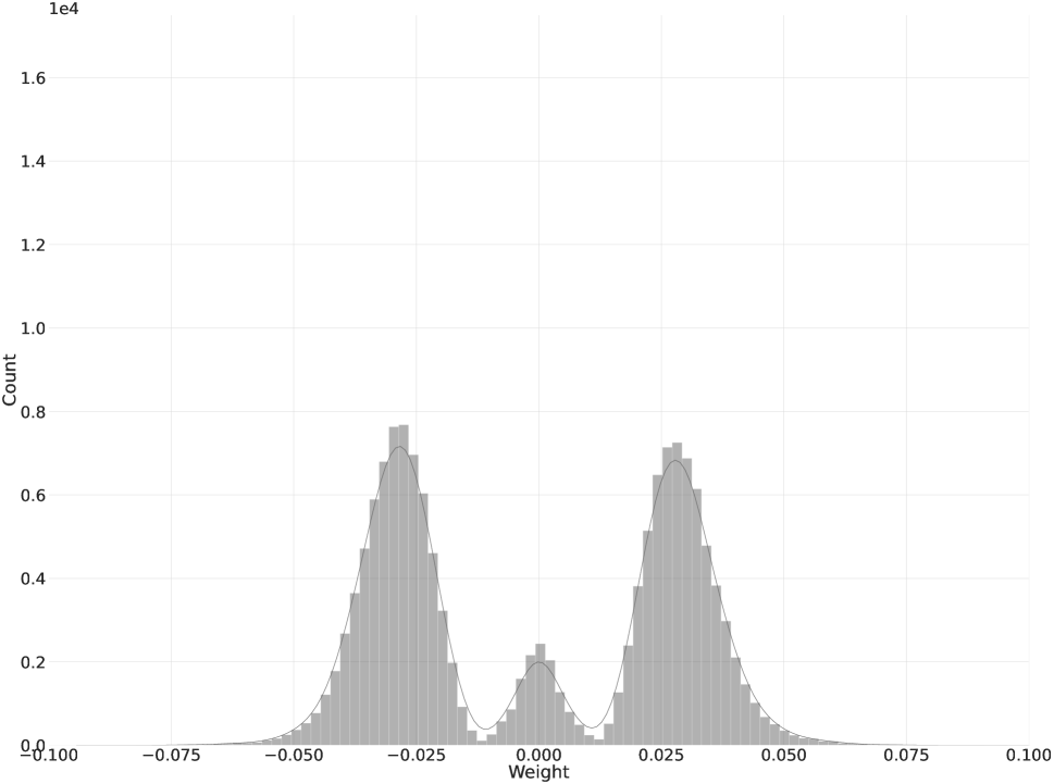
where $t$ controls the sparsity, i.e., percentage of zero values, of $\mathbf{\hat{W}}$ (Figure 1), and $\texttt{ValueAtIndex}([\cdot],\texttt{idx})$ returns a value of $[\cdot]$ at the index idx. During training, based on the work of (liu2018rethinking), we initially assign $t=0.5$, namely, removing $50\%$ values by their magnitude in $\mathbf{W}$ as the potential ternary references $\mathbf{\hat{W}}$, then $t$ is gradually increased to $t=0.7$, i.e., 70% of $\mathbf{\hat{W}}$ is zero. We use the quadratic term to keep $L(\mathbf{W})$ and $L_{d}(\mathbf{W},\Delta)$ at the same scale. Since $J(\mathbf{W})$ consists of two parts and is optimized in continuous space, the distance between $\mathbf{W}$ and $\mathbf{\hat{W}}$ will gradually decrease without much change in model accuracy. In practice, we observe that applying $L_{d}(\mathbf{W},\Delta)$ barely reduces the model accuracy.

Since we are training with hyperspherical settings, i.e., $\|\mathbf{w}_{j}\|_{2}=\|\mathbf{\hat{w}}_{j}\|_{2}=1$, the diagonal elements of $\mathbf{W}^{\top}\mathbf{\hat{W}}$ in Eq. (7) denotes the cosine similarities between $\mathbf{w_{j}}$ and $\mathbf{\hat{w}_{j}}$. Minimizing $L_{d}$ is equivalent to pushing $\mathbf{w}_{j}$ close to $\mathbf{\hat{w}}_{j}$, namely, making part of the magnitude of weight values close to $\alpha$ (Eq. (4)) while the rest close to zero (Figure 1). In addition, the gradient of $L_{d}$ can adjust $\frac{\partial J}{\partial{\mathbf{W}}}$, which is similar to the works of (hou2018loss_31; yang2019quantization_22; zhou2018explicit_26.5; dbouk2020dbq_20).

With $\mathbf{W}$ getting close to $\hat{\mathbf{W}}$ before the ternary quantization, we still need to convert the full precision weight to ternary values. We change the $\Delta$ to a learnable threshold $\bar{\Delta}$ and empirically initialize $\bar{\Delta}=\texttt{T}(t+0.1)$ via Eq. (8). The Eq. (6) becomes:

We introduce a gradient scaling factor $S$ and adopt STE (bengio2013estimating) to bypass the non-differentiable problem of $\texttt{Ternary}(\cdot)$:

Forward:

Backward:

where $S$ is defined as:

and $\odot$ denotes the element-wise multiplication. Inspired by the work of (yang2019quantization_22), $1-w^{2}$ is used to re-scale the gradient of $w_{ij}$ as it shares similarities with the derivative of $\texttt{Sigmoid}(\cdot)$ (Figure 2). $S$ is intuitive and easy to calculate. The gradient of $w_{ij}$ should be smaller when it gets farther away from $\bar{\Delta}$. This intuition is the same as the works of (hou2018loss_31; zhou2018explicit_26.5; dbouk2020dbq_20).

We simply apply the averaged gradients of $w_{ij}$ to update the quantization threshold $\bar{\Delta}$:

Figure 1 shows that we can initialize $\bar{\Delta}$ with a smaller value and then gradually increase it until the near-zero portion is converted to zero during quantization. We should increase the threshold $\bar{\Delta}$ rapidly when the error is very large. As the training error becomes smaller, such increase should slow down.

For image classification, the batch size is 256. The weight decay is 0.0001, and the momentum of stochastic gradient descent (SGD) is 0.9. We use the cosine annealing schedule with restarts (loshchilov2016sgdr) to adjust the learning rates. The initial learning rate is 0.01. All of the experiments use 16-bit Automatic Mixed Precision (AMP) from PyTorch to accelerate the training process. The first convolutional layer and last fully-connected layer are skipped when quantizing ResNet models. For the MobileNetV2, and Mask R-CNN, we only skip the first convolutional layer.