Hyperuniformity and phase separation in biased ensembles of trajectories for diffusive systems
Abstract
We analyse biased ensembles of trajectories for diffusive systems. In trajectories biased either by the total activity or the total current, we use fluctuating hydrodynamics to show that these systems exhibit phase transtions into ‘hyperuniform’ states, where large-wavelength density fluctuations are strongly suppressed. We illustrate this behaviour numerically for a system of hard particles in one dimension and we discuss how it appears in simple exclusion processes. We argue that these diffusive systems generically respond very strongly to any non-zero bias, so that homogeneous states with “normal” fluctuations (finite compressibility) exist only when the bias is very weak.
pacs:
05.40.-aIntroduction – Non-equilibrium systems exhibit diverse collective behaviour and complex emergent phenomena, many of which have no counterparts at equilibrium. Even in simple interacting particle systems, one may encounter long-ranged correlations spohn83 , dissipative “avalanche” events with no typical size btw , and dynamical phase transitions bodineau2004 ; garrahan2007 . Theories that capture the universal aspects of these fluctuations are much sought-after, as a route to general descriptions of non-equilibrium phenomena. Here, we analyze non-equilibrium ensembles of trajectories bodineau2004 ; lecomte2005 ; garrahan2007 , defined through constraints on macroscopic observables such as the total current or activity within a given time period. Phase transitions within these ensembles occur when such a constraint leads to a qualitative change in macroscopic behaviour bodineau2004 ; garrahan2007 ; bodineau2008 ; hedges2009 . In diffusive systems bertini2001 ; bertini2005 ; tkl2007 ; hurtado2011-pnas ; bertini-revs , we demonstrate transitions into “hyperuniform” (HU) states torquato2003 , as well as transitions into the macroscopically inhomogeneous (“phase separated”) states that have previously been found bodineau2004 ; bodineau2008 . Hyperuniform states are characterised by anomalously small density fluctuations on large length scales torquato2003 ; florescu2009 ; zachary2011 ; berthier2011 ; man2013 ; chicken2014 ; levine-arxiv ; they have been identified in jammed particle packings berthier2011 ; zachary2011 and in biological systems chicken2014 . These systems are highly optimised in response to a global constraint (mechanical stability in jamming, optimal fitness in biology). The constrained dynamical ensembles that we consider in this study are also optimised: they are the maximally probable states consistent with the constraint. Our results (i) provide further evidence that hyperuniformity is generic, by demonstrating that it occurs in a new set of optimised non-equilibrium ensembles, and (ii) resolve the physical interpretation of some phase transitions that have been previously discovered in diffusive systems appert2008 ; bodineau2008 .
Models – We study biased ensembles of trajectories both computationally and analytically. For computational studies, we consider a one-dimensional model of diffusing hard particles in a periodic box of size , with each particle having size . This Brownian hard-particle model (BHPM) evolves by Langevin dynamics: the position of particle obeys where the are independent white noises, is the potential energy, and the inverse temperature. The diffusion constant of an isolated free particle is . We use a Monte Carlo (MC) dynamical scheme to simulate this system. Full system details are given in Appendix A.
We also consider lattice-based exclusion models where particles are distributed over lattice sites, again with periodic boundaries. At most one particle may occupy any lattice site. In the partially asymmetric simple exclusion process (PASEP), particles hop left with rate and right with rate , provided their destination site is empty. The symmetric simple exclusion process (SSEP) is the case . The steady states of the BHPM and the PASEP have no correlations between particles beyond hard-core exclusion. (Unlike the SSEP and BHPM, the PASEP does not obey detailed balance, but for periodic boundaries, it may still be shown that site occupancies are uncorrelated in the steady state.)
Biased ensembles of trajectories – Let be a measure of dynamical activity in a trajectory . For exclusion processes, is the total number of particle hops in a trajectory. For the BHPM, we follow hedges2009 : we choose a coarse-graining time and focus on trajectories of length , defining with . The position is defined by subtracting the centre-of-mass motion (see Appendix A) which helps to minimize finite-size effects. We take , in which time an isolated particle diffuses a distance comparable with its size. We fix the units of time by setting .
To investigate trajectories that are constrained to non-typical values of , we define a biased ensemble of trajectories spohn1999 ; lecomte2005 ; garrahan2007 , via a formula for the average of an observable :
| (1) |
Here represents an average in the (unbiased) steady state of the model, is an average within the biased ensemble, and is a ‘dynamical free energy’. For sufficiently large , averages in the biased ensemble are equal to averages over trajectories in which the activity is constrained touchette2013 .
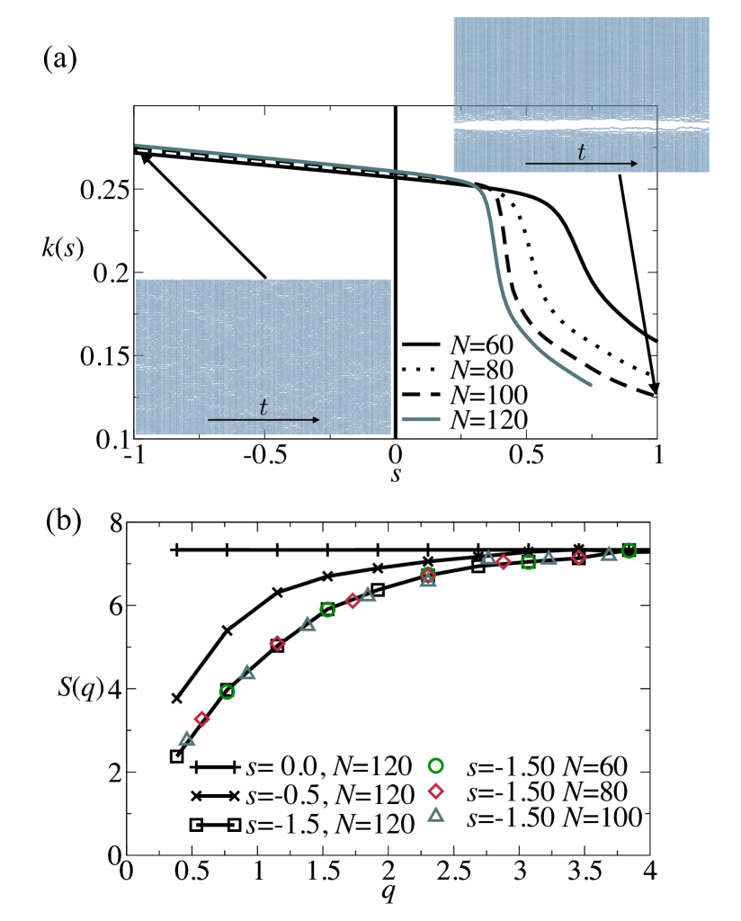
Numerical results for the BHPM – Fig. 1 has results for the BHPM, calculated using transition path sampling tps ; hedges2009 . Fig. 1(a) shows the mean activity . For there is a first-order transition into a phase separated state bodineau2004 ; bodineau2008 ; lecomte2012 . For , the activity appears to depend smoothly on , but the system develops strong long-ranged correlations. These are measured by the structure factor where and , with the mean density. To see the relevant behavior most clearly, we transform co-ordinates so that the particles are treated as point-like (see Appendix A): defining , the equilibrium () ensemble then has , independent of . Fig. 1(b) shows that for and small , the structure factor deviates strongly from this equilibrium value. The signature of a hyperuniform state is that at small- torquato2003 : density fluctuations on large length scales are strongly suppressed. This means that particle positions necessarily have long-ranged correlations [otherwise, self-averaging of the density within large regions of the system implies ]. Analysis of the small- behaviour in numerical simulations is limited by the system size, but the results for are consistent with hyperuniformity.
Fluctuating hydrodynamics – The BHPM is representative of a general class of diffusive systems, which may be described by “fluctuating hydrodynamics” spohn83 ; eyink1990 ; bertini-revs . Within this theory, the time-evolution of the density on large length and time scales can be approximated by a Langevin equation
| (2) |
where is a white noise, and are local measures of diffusivity and mobility, and is an asymmetric driving force. Details of the relationships between fluctuating hydrodynamics and the BHPM, SSEP and PASEP are given in Appendix B. Note that the fluctuating hydrodynamic theory is valid in all dimensions, not just .
Hyperuniformity within fluctuating hydrodynamics – Consider a system described by (2) with , and introduce a bias to larger-than-average activity, . Averages within the biased ensemble are given by path-integral expressions: , where is a (real-valued) response field, and
| (3) |
in which is the (density-dependent) local activity of the system. We assume , which certainly holds for exclusion processes and may be expected to hold for generic particle systems; analysing the case with is also straightforward kmp ; lecomte2010 ; hurtado-rev . The behavior of for the BHPM is shown in Appendix A.
Analysis of hydrodynamic behaviour requires a suitable rescaling of space and time co-ordinates. To avoid cumbersome notation we defer this procedure to Appendix B and quote our results in terms of the bare (unrescaled) parameters. Note, however, that these results apply only in the hydrodynamic limit. For , the path integral is dominated by trajectories where and so we write and expand to quadratic order in and . The result is
| (4) |
where we write , with , etc, and similarly for and .
The structure factor may then be evaluated (see (bodineau2008, , Equ. (58)) and also Appendix B, yielding
| (5) |
We again emphasise that this result is valid only for small , and that , by assumption.
Equ. (5) demonstrates a singular response to the field . For and , the structure factor approaches a non-zero constant , as expected in an equilibrium state with a finite compressibility. However, for any , the large scale behaviour changes qualitatively: . The numerical results of Fig. 1(b) are consistent with this theoretical prediction. Note that hyperuniformity is a large length scale phenomenon: the non-trivial behaviour in appears only for small .
We also calculate the mean activity . Writing , we see that the suppression of at small acts to increase [recall ]. Taking and , we obtain (see appert2008 and also Appendix B):
| (6) |
which is valid to leading order in . Since where is the dynamical free energy, we identify this non-analytic behaviour in with a second order dynamical phase transition. This singular behavior has been noted before appert2008 , but its link with hyperuniformity has not. In , the suppression of at small wavevectors leads to a singular contribution , with logarithmic corrections if is even (see Appendix B). As illustrated in Fig. 1, biasing to lower-than-average activity by choosing instead leads to phase separation bodineau2004 ; bodineau2008 ; lecomte2012 ; hurtado-rev .
Heuristic explanations for HU states – The origin of hyperuniformity in biased diffusive systems is the diverging hydrodynamic time scale associated with large-scale density fluctuations. To see this, consider linear response to the field . Within a biased ensemble of trajectories, the probability of finding the system in a configuration is where is a “propensity” propensity , which is obtained by averaging the activity over trajectories that start in at , and comparing with typical equilibrium trajectories garrahan2009 ; jack2014-east .
If has an unusual density fluctuation at a small wavevector , expanding to quadratic order in gives . Diffusive scaling therefore indicates that , where is a relaxation time, is the amplitude of the density fluctuation and the structure factor of the unbiased state. In hyperuniform states we expect yielding : the time scale diverges for large and , so these are strongly enhanced for . On the other hand, phase-separated configurations have and so : these configurations have strong (divergent) enhancement for and as . Hence, this perturbative analysis reveals an instability of the small- modes to changes in : we argue that this is the origin of the HU and phase-separated states when . The diverging diffusive time scale is central to this analysis, similar to other cases where diverging time scales lead to phase transitions in biased ensembles jack2010rom ; garrahan2009 .
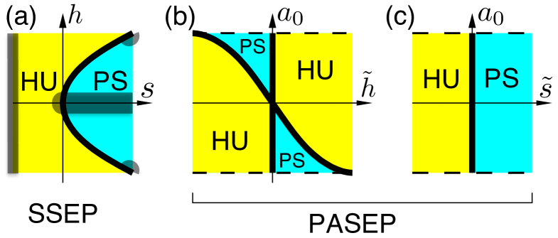
Biased ensembles based on the total current – So far, we have considered ensembles of trajectories biased according to their activity . In fact, HU states also appear in ensembles of trajectories where the total current is biased. We define the total current as the sum of all (directed) particle displacements in a trajectory. (For exclusion processes, this is the difference between the numbers of right- and left- hops.) For generality, we consider jointly-biased ensembles where the activity is biased by a field and the current is biased by a field . The analogue of (1) is (see Appendix B). Within fluctuating hydrodynamics and assuming a time-reversal symmetric unbiased state () one finds that the response to the bias depends only on the quantity (see Appendix B). For then has a finite (non-zero) limit as ; for the system is HU while for one has phase separation. The resulting dynamical phase diagram is shown in Fig. 2: the fluctuating hydrodynamic analysis holds only for , but in the absence of additional phase transitions one expects the same structure to hold throughout the -plane. We discuss this conjecture below, using results from exclusion processes. We also note in passing that the centre of mass in the BHPM undergoes free diffusion so that the distribution of the current is trivial in that case: in the fluctuating hydrodynamic theory, this means that , so .
The condition [solid line in Fig. 2(a)] recovers a homogeneous state with : we use the term “normal fluctuations” for this case, in contrast to hyperuniform or phase-separated states. In fact, biased ensembles with are identical to (unbiased) steady states of models in which time-reversal symmetry is broken (). This may be verified directly from the hydrodynamic Lagrangian (3) but a clearer interpretation of this result can be obtained by analyzing exclusion processes, as we now discuss.
Mappings between biased ensembles for exclusion processes – We analyse exclusion processes via operator representations of their master equations stinch-review . Starting from the master equation for the SSEP, we write a biased generator spohn1999 ; lecomte2005 that describes the jointly biased ensemble. This operator has a representation in terms of Pauli spin matrices tkl2008 (see Appendix C)
| (7) |
where . If we consider instead a PASEP biased by its current, the relevant operator is , where are hopping rates and the biasing field. For appropriate parameters (including always the normalization ), we may have , which means that the trajectories of the two biased ensembles are identical. Defining the hopping asymmetry , equality between and requires and . Any jointly-biased SSEP with leads to two solutions for , which correspond to two possible current-biased PASEPs. These two possibilities are related by a Gallavotti-Cohen symmetry gallavotti-cohen ; spohn1999 . In the specific case [so that ], one has : the Gallavotti-Cohen symmetry relates biased and unbiased PASEP states, both of which have “normal” fluctuations.
The SSEP with is another special case, because it leads to : the steady state of a jointly-biased SSEP corresponds exactly to that of an unbiased PASEP. This is the microscopic interpretation of the condition in the fluctuating hydrodynamic analysis [for small , we obtain which is consistent with , because for the SSEP]. The unbiased steady state of the PASEP has normal fluctuations”, so we conclude that fluctuations are also normal along the line in the dynamical phase diagram of the jointly-biased SSEP [solid line in Fig. 2(a)].
There are a family of mappings between biased SSEPs and PASEPs (see Appendix C): for example, an activity-biased PASEP may also be mapped to a jointly-biased SSEP. The resulting situation is shown in Fig. 2(b,c) where we show the PASEP dynamical phase diagrams that correspond to the (conjectured) phase diagram in Fig. 2(a). The hypothesis is that all points in Fig. 2(a) are either phase separated (PS) or hyperuniform (HU), except for the normal line . We provide several arguments in support of this picture. The fluctuating hydrodynamic analysis establishes these results in the small bias regime, , since the condition then reduces to the case discussed above. The question is therefore whether some other phase transition might intervene and destroy the PS or HU correlations when .
We are not able to rule out this possibility but several exact results indicate strongly that there is no such phase transition. (i) For , the density correlations of the PASEP are known popkov2011 : independently of the asymmetry , there is a logarithmic effective interaction potential between particles which renders this state hyperuniform. This implies that the jointly-biased SSEP is HU as (for all ). (ii) For , a variational argument garrahan2007 indicates that the SSEP phase separates for all : the system can then access configurations where the total number of available hops remains finite as . (iii) Phase separation has been shown analytically for the totally asymmetric exclusion process (): this transition corresponds to the appearance of “shocks” in response to a bias on the current bodineau2005 . For the SSEP, this establishes phase separation for all in the limit . Combining these results establishes that the proposed phase diagram of Fig. 2(a) is correct in all of the shaded regions: we cannot rule out other phase diagrams that are consistent with these constraints but this simple picture is the most likely scenario. If the proposed Fig. 2(a) is correct, the phase diagrams in Fig. 2(b,c) follow from the exact mappings between biased SSEP and PASEPs.
Conclusion – Fig. 2 indicates that exclusion processes respond very strongly to biases and , which almost always lead to either phase-separated or hyperuniform states. The normal fluctuations that are familiar from equilibrium systems occur only under special high-symmetry conditions, such as . These results provide another example zachary2011 ; chicken2014 ; levine-arxiv of hyperuniformity emerging in non-equilibrium states, and they show that the dynamical phase transition identified in appert2008 corresponds physically to the appearance of hyperuniformity. More generally, the theory of fluctuating hydrodynamics indicates that these dynamical phase transitions should be generic (“universal”) in systems with locally-conserved hydrodynamic variables such as energy or density. The interplay between these phase transitions and the “glass transitions” found previously in biased ensembles of trajectories garrahan2007 ; garrahan2009 ; hedges2009 merits further study – diffusive large-scale behaviour is not a necessary condition for those glass transitions garrahan2007 ; elmatad2010 , but the analysis presented here indicates that phase-separated states may compete with homogeneous glassy states in systems that are biased to low activity.
We thank Fred van Wijland, Vivien Lecomte, and Juan P. Garrahan for many useful discussions. RLJ and IRT were supported by the EPSRC through grant EP/I003797/1.
References
- (1) H. Spohn, J. Phys. A 16, 4275 (1983)
- (2) P. Bak, C. Tang and K. Wiesenfeld, Phys. Rev. Lett. 59, 381 (1987).
- (3) T. Bodineau and B. Derrida, Phys. Rev. Lett. 92, 180601 (2004).
- (4) J. P. Garrahan, R. L. Jack, V. Lecomte, E. Pitard, K. van Duijvendijk and F. van Wijland, Phys. Rev. Lett. 98, 195702 (2007)
- (5) V. Lecomte, C. Appert-Roland and F. van Wijland, Phys. Rev. Lett. 95, 010601 (2005)
- (6) T. Bodineau, B. Derrida, V. Lecomte and F. van Wijland, J. Stat. Phys. 133, 1013 (2008).
- (7) L. O. Hedges, R. L. Jack, J. P. Garrahan and D. Chandler, Science 323, 1309 (2009).
- (8) L. Bertini, A. De Sole, D. Gabrielli, G. Jona-Lasinio, and C. Landim, Phys. Rev. Lett. 87, 040501 (2001); J. Stat. Phys. 107, 625 (2002).
- (9) L. Bertini, A. De Sole, D. Gabrielli, G. Jona-Lasinio, and C. Landim, Phys. Rev. Lett. 94, 030601 (2005).
- (10) J. Tailleur, J. Kurchan and V. Lecomte, Phys. Rev. Lett. 99, 150602 (2007)
- (11) P. I. Hurtado, C. Perez-Espigares, J. J. del Pozo and P. L. Garrido, PNAS 108, 7704 (2011)
- (12) L. Bertini, A. De Sole, D. Gabrielli, G. Jona-Lasinio and C. Landim, J. Stat. Phys. 135, 857 (2009); arXiv:1404.6466 (2014)
- (13) S. Torquato and F. H. Stillinger, Phys. Rev, E 68, 041113 (2003).
- (14) M. Florescu, S. Torquato and P. J. Steinhardt, PNAS 106, 20658 (2009)
- (15) C. E. Zachary, Y. Jiao and S. Torquato, Phys. Rev. Lett. 106, 178001 (2011)
- (16) L. Berthier, P. Chaudhuri, C. Coulais, O. Dauchot and P. Sollich, Phys. Rev. Lett. 106, 120601 (2011)
- (17) W. Man, M. Florescu, K. Matsuyama, P. Yadak, G. Nahal, S. Hashemizad, E. Williamson, P. Steinhardt, S. Torquato and P. Chaikin, Optics Express 21, 19972 (2013).
- (18) Y. Jiao, T. Lau, H. Hatzikiriou, M. Meyer-Hermann, J. C. Corbo and S. Torquato, Phys. Rev. E 89, 022721 (2014)
- (19) D. Hexner and D. Levine, arXiv:1407.0146.
- (20) J. Tailleur, J. Kurchan and V. Lecomte, J. Phys. A 41, 505001 (2008)
- (21) C. Appert-Rolland, B. Derrida, V. Lecomte and F. van Wijland, Phys. Rev. E 78, 021122 (2008)
- (22) J. L. Lebowitz and H. Spohn, J. Stat. Phys. 95, 333 (1999).
- (23) R. Chétrite and H. Touchette, arXiv:1405.5157.
- (24) P. G. Bolhuis, D. Chandler, C. Dellago and P. L. Geissler, Ann. Rev. Phys. Chem. 53, 291 (2002).
- (25) V. Lecomte, J. P. Garrahan and F. van Wijland, J. Phys. A 45, 175001 (2012).
- (26) P. I. Hurtado, C. P. Espigares, J. J. del Pozo, P. L. Garrido, J. Stat. Phys. 154, 214 (2014)
- (27) G. L. Eyink, J. Stat. Phys. 61, 533 (1990).
- (28) C. Kipnis, C. Marchioro, E. Presutti, J. Stat. Phys. 27, 65 (1982).
- (29) V. Lecomte, A. Imparato, and F. van Wijland, Prog Theor Phys. Supp. 184, 276 (2010).
- (30) A. Widmer-Cooper, P. Harrowell and H. Fynewever, Phys, Rev. Lett. 93 135701 (2004).
- (31) J. P. Garrahan, R. L. Jack, V. Lecomte, E. Pitard, K. van Duijvendijk, and F. van Wijland, J. Phys. A 42, 075007 (2009).
- (32) R. L. Jack and P. Sollich, J. Phys. A 47, 015003 (2014).
- (33) R. L. Jack and J. P. Garrahan, Phys. Rev. E 81, 011111 (2010).
- (34) R. Stinchcombe, Adv. Phys. 50, 431 (2001).
- (35) G. Gallavotti and E. G. D. Cohen, J. Stat. Phys. 80, 931 (1995).
- (36) V. Popkov and G. M. Schütz, J. Stat. Phys. 142, 627 (2011).
- (37) T. Bodineau and B. Derrida, Phys. Rev. E 72, 066110 (2005).
- (38) Y. S. Elmatad, R. L. Jack, J. P. Garrahan and D. Chandler, PNAS 107, 12793 (2010).
- (39) P. C. Martin, E. D. Siggia and H. A. Rose, Phys. Rev. A 8, 423 (1973); C. De Dominicis, Lett. Nuovo Cimento, 12, 567 (1975); H.-K. Janssen, Z. Phys. B 23, 377 (1976).
- (40) A. B. Bortz, M. H. Kalos and J. L. Lebowitz, J. Comp. Phys. 17, 10 (1975); M. E. J. Newman and G. T. Barkema, Monte Carlo Methods in Statistical Physics, (OUP, Oxford, 1999).
Appendix A Appendix A:
BROWNIAN HARD-PARTICLE MODEL
In the Brownian hard-particle model, there are particles with positions , in a box of size , with periodic boundaries. Since the particles are hard, they do not overtake one another, so we assign particle indices such that . According to the Langevin dynamics, the centre of mass undergoes free diffusion with diffusion constant . When evaluating the dynamical activity , we use
In cases where the particle travels around the periodic boundaries of the system, the position is defined so that it varies continuously, so we may have or ; for the purposes of particle interactions, we use the position of the particle within the box, which is .
It is convenient to define where is the particle size. The diffuse in a periodic box of size ; in the equilibrium state, they are distributed independently and uniformly throughout the box. If particle indices are ignored, the trajectories of the are the same as those of independent freely diffusing particles (with no hard-core interaction). This mapping is valid because in terms of the density field, a “collision” between two particles has the same effect as two particles diffusing past each other. This means that multi-point space-time correlations of the density can in principle be calculated exactly. However, the activity requires that we keep track of particle indices and collisions. This means that the activity fluctuations in the model are not trivial, as is clear from Fig. 1.
When evaluating the structure factor for the BHPM we use the definition with and integer, so that at equilibrium (), independent of . We argue that this structure factor has the same small- behaviour as the structure factors calculated directly from the particle positions , as follows. The structure factor for small can be inferred from the fluctuations of the number of particles within regions (subsystems) of size . The ‘hat’ notation indicates that is a fluctuating quantity. For a homogeneous system, and assuming that is much larger than the particle spacing, we can equivalently consider the size of a subsystem (or region) containing exactly particles. If we take then we expect
| (8) |
At equilibrium, this relation is most easily proved via correlation-response formulae for the isothermal compressibility, but we argue here that it also holds in the out-of-equilibrium states found in biased ensembles. To see this, define a local density , which may either be written as or obtained equivalently as . The variance of the local density may then be written either in terms of or . We assume (based on a self-averaging argument) that for large the fluctuations of are small, from which we obtain (8). Finally, we note that if is the size of the hard particles then the probability distribution of satisfies , where is the distribution for particles of size and is the distribution for point-particles. Hence is equal in both representations, which is sufficient to establish that the structure factors are equal (up to a multiplicative constant).
To simulate the BHPM, we use a Monte Carlo (MC) scheme: in each MC move a particle is chosen at random and a displacement is chosen uniformly between and . The move is rejected if moving the particle to involves a particle overlap, otherwise it is accepted. For small , this scheme is equivalent to solving the Langevin dynamics of the interacting particles; a time in the Langevin system corresponds to attempted MC moves per particle. We take . For the relatively high density () relevant for Fig. 1, it is convenient to use a continuous-time implementation of these dynamics in which all moves are accepted BKL .
Appendix B Appendix B: FLUCTUATING HYDRODYNAMICS
B.1 Relation to microscopic models
The relation between fluctuating hydrodynamic equation (2) and microscopic models has been discussed in several previous studies bertini2001 ; tkl2008 ; appert2008 ; bertini-revs . The SSEP corresponds to fluctuating hydrodynamics with , and (see for example appert2008 , and note we have unit rates for both left and right hops). For the PASEP, the fluctuating hydrodynamic theory applies only for the weakly-asymmetric model (sometimes called the WASEP), in which case , and the theory applies only for very small .
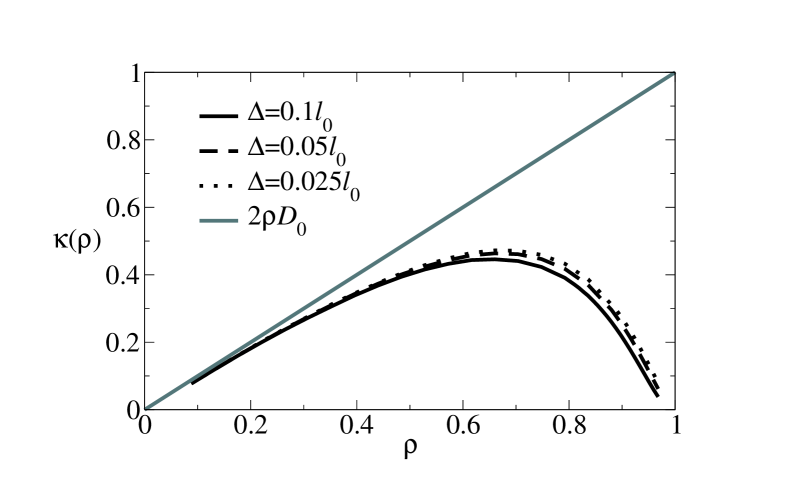
In the BHPM, the behaviour of the unbiased model corresponds to and ; it is useful to compare with the small- limit of the SSEP, which reduces to the BHPM after a suitable rescaling of time. The function is not known analytically: we show numerical data in Fig. 3 from which we see that , as stated in the main text.
B.2 Rescaled co-ordinates
We take the hydrodynamic limit by rescaling lengths by a large (dimensionless) factor , so our system of size maps into a box of size . Typically one fixes and takes but it will be convenient in the following to take first and then later . Let and , and because has dimensions of a rate (inverse time) also . Let and similarly .
Then the action in the path integral representation of the dynamics is with given to quadratic order by (4), so that
| (9) |
where the approximate equality emphasises that we have truncated at quadratic order. (Here acts on the rescaled co-ordinate: we omit the variable being used where this is unambiguous from the context.)
Transforming to the Fourier domain, we write . The inverse transform is . The key point is that the theory is evaluated with fixed cutoffs and which are of order unity as . This ensures (for example) that loop corrections can always be neglected in perturbative calculations. (The allowed wavectors are for integer and similarly .)
B.3 Activity bias
To analyze the effect of the bias , we start from (9). We can write the action as
| (10) |
with (to quadratic order)
| (11) |
To calculate the structure factor, we must consider the integral . Making a saddle-point approximation, the behaviour depends only on the quadratic-order expansion (11), and we obtain
| (12) |
To obtain the equal-time fluctuations we define , with . We have : taking before any limit of large-, the sum over may be converted to an integral. As long as the frequency cutoff satisfies , we obtain
| (13) |
While the derivation of this equation required a saddle-point approximation [equivalent to the truncation at quadratic order in (9)], it can be shown that this approximation becomes exact in the limit of large-. Finally, converting from the rescaled parameters , , to the bare quantities , , yields (5) of the main text. The requirement that be large while and are of order unity implies that (5) is valid only for very small and , as discussed in the main text.
B.4 Current bias
Now suppose that, instead of coupling to activity, we couple to the particle current . Within fluctuating hydrodynamics, we write with . Using the method of Martin-Siggia-Rose-DeDominicis-Janssen msr ; tkl2008 , we arrive at a path integral with Lagrangian
| (14) |
The system has periodic boundaries: if we assume (as expected) that for some , the last term in (14) vanishes after integration over .
Expanding about the homogeneous stationary profile as in the activity-biased case, the analogue of (4) of the main text is
| (15) |
Stability of the homogeneous profile requires , which is the case for exclusion processes and the BHPM. To proceed, we rescale co-ordinates as in the previous section, defining in addition . The calculation is almost identical so we give only a brief discussion: we find
| (16) |
To obtain the structure factor, we perform a frequency integral, and the term plays no role since it can be absorbed by a shift of the integration variable. Hence we arrive at the result for the structure factor (in terms of the bare variables):
| (17) |
(Note , by assumption.) This is the same form as (5) of the main text, but with and . Hence, as long as , the effect of the current bias is the same as the bias to higher-than-average activity, .
B.5 Joint bias
The analysis for a joint bias on activity and current is a trivial extension of the previous cases. Assuming a homogeneous state, we obtain
| (18) |
with . The self-consistency condition for homogeneity is . The similarity with (16) allows straightforward calculation of the structure factor in these ensembles.
B.6 Scaling of for
We now show how the activity can be calculated within fluctuating hydrodynamics. The relevant expression is given by expanding to quadratic order in :
| (19) |
Hence, working at quadratic order
| (20) |
We define : in terms of the rescaled hydrodynamic variables, we obtain
| (21) |
Taking at fixed , we can convert the sum to an integral arriving at
| (22) |
It is convenient to define , so .
For we obtain
| (23) |
The leading term is non-analytic at (which corresponds to ): in terms of the bare parameters, this gives the result quoted in the main text.
For , the integral gives a singular behaviour proportional to in odd dimensions, and in even dimensions. There are also analytic “non-universal” (-dependent) terms that lead to a polynomial dependence on . For example in
| (24) |
where the leading behaviour at small is a non-universal term at but the first singular contribution is the universal contribution from small wavevectors. Similarly for ,
| (25) |
The behavior in higher dimensions can be obtained analogously by repeated integration by parts, starting from (22).
Appendix C Appendix C:
EXACT MAPPINGS FOR EXCLUSION PROCESSES
As in the main text the jointly biased SSEP (with periodic boundaries) is associated with an operator spohn1999 ; lecomte2005 ; appert2008
| (26) |
Similarly, the relevant operator for the current-bisaed PASEP is
| (27) |
Note the Gallavotti-Cohen symmetry gallavotti-cohen ; spohn1999 : setting recovers the original unbiased model but with the opposite bias.
For correspondence with the jointly biased SSEP we require and , as well as . Hence and . Adding gives : the case reduces to an unbiased PASEP. For small , this means which corresponds to the condition in analysis of fluctuating hydrodynamics. The general mapping from SSEP to current-biased PASEP requires , and there are typically two solutions for : each point in the right half plane of Fig. 2(a) therefore maps to two points in Fig. 2(b), one with and the other with .
If we instead consider an activity-biased PASEP, the relevant operator is
| (28) |
For correspondence with we require and and again . Taking the first and third of these gives the asymmetry parameter as : the current bias on the SSEP sets the asymmetry of the PASEP. On the other hand, taking the first and second constraints, and and given we have . As before, we recover an unbiased PASEP if .
The general case of a PASEP with a joint bias on current and activity is a simple generalisation. Given that we have fixed the time unit in the SSEP so that the coefficient of the diagonal term is always , the jointly biased SSEP is a two-parameter family of models dependent on . Fixing the time unit in the PASEP in the same way, the jointly biased PASEP has parameters: . However, the only free parameters for the relevant operator are the coefficients of the and terms. Hence every jointly biased SSEP can be mapped into a one-parameter family of PASEPs.
We note that these mappings also hold in if the activity bias couples to the total number of hops along just one Cartesian direction.
C.1 Weak asymmetry and fluctuating hydrodynamics
The mapping between jointly biased SSEP and the unbiased weakly-asymmetric exclusion process (WASEP) can also be accomplished at the fluctuating hydrodynamic level. E.g. for a WASEP with asymmetry-parameter the Lagrangian is
| (29) |
Integrating by parts on the term with just one gradient and then completing the square yields
| (30) |
This a jointly biased SSEP with a current-bias and an activity bias [we have ] so that . This is consistent with the fact that any unbiased WASEP has normal fluctuations, so must lie on the line .