44email: *wadduwage@fas.harvard.edu
Hypothesis-Driven Deep Learning for Out of Distribution Detection
Abstract
Predictions of opaque black-box systems are frequently deployed in high-stakes applications such as healthcare. For such applications, it is crucial to assess how models handle samples beyond the domain of training data. While several metrics and tests exist to detect out-of-distribution (OoD) data from in-distribution (InD) data to a deep neural network (DNN), their performance varies significantly across datasets, models, and tasks, which limits their practical use. In this paper, we propose a hypothesis-driven approach to quantify whether a new sample is InD or OoD. Given a trained DNN and some input, we first feed the input through the DNN and compute an ensemble of OoD metrics, which we term latent responses. We then formulate the OoD detection problem as a hypothesis test between latent responses of different groups, and use permutation-based resampling to infer the significance of the observed latent responses under a null hypothesis. We adapt our method to detect an unseen sample of bacteria to a trained deep learning model, and show that it reveals interpretable differences between InD and OoD latent responses. Our work has implications for systematic novelty detection and informed decision-making from classifiers trained on a subset of labels.
Keywords:
Novelty Detection, Deep Learning, Model Generalization, Model Interpretability1 Introduction
There is an increasing trend of using black-box machine learning (ML) for high-stakes prediction problems that deeply affect human lives, such as healthcare. Deep learning models inherently provide no explanation of their predictions in a human-interpretable manner. Deploying such models despite the lack of transparency and accountability can have (and already has) severe consequences [10]. Such problems are worsened when models are only trained on a small subset of the target population. For instance, when training black-box models to diagnose bacterial infections, it is infeasible to collect data spanning the entire population of bacteria species, so only a small subset of bacterial species is used instead [3, 4]. Formally, given a population of bacteria species, the common approach is to sample species (), train a classifier within that subset, and report their performance on unseen samples from the species themselves. Such classifiers, if deployed in the real-world, are bound to receive inputs that appear similar to the training data, but are outside the species. Thus, a classifier untested on samples beyond the species may perform unpredictably on real-world data, which makes them unsafe for clinical use. To mitigate such problems, we require trustworthy models that not only classifies samples from known categories well, but also detects when samples cannot be assigned to those categories [2]. For instance, a trustworthy digit classifier should not only classify digit inputs correctly, but allow to detect non-digit inputs and reject them instead of blindly classifying them into existing categories.
Hypothesis testing is a fundamental concept in statistics that allows us to draw conclusions about an entire population based on a representative sample. At its core, hypothesis testing involves making assumptions about population parameters and then rigorously assessing whether the sample data provides enough evidence to support or reject these assumptions. In this paper, we reformulate the OoD detection problem as a hypothesis test, where we check for differences in OoD metrics between InD and OoD groups through a resampling approximation of the null distribution. The OoD metrics are chosen depending on a model’s inductive biases, and our test is independent of this choice. Further, we propose a technique based on leave-out training to quantify a model’s discriminating power for near-OoD inputs (i.e., same domain, different class). We test our method on several model architectures, datasets, and label splits, and show that it quantifies differences between InD and OoD data in an interpretable way. Overall, our method provides a basis for making informed decisions from classifiers trained on a subset of labels.
2 Related Work
2.1 Out of Distribution Detection
Out-of-Distribution (OoD) detection is the idea of detecting inputs that do not match the training data distribution of a given model [13]. Recent work on OoD detection include improved OoD metrics [12], OoD detection tests [7, 9], OoD aware training procedures [11], and post-hoc calibration procedures [5]. While a plethora of OoD metrics and tests exist, their discriminative power varies across model architectures and the nature of OoD data in the target domain [13]. We posit that an ensemble of OoD metrics could provide more discriminative power than a single metric.
2.2 Multi-Response Permutation Procedure (MRPP)
MRPP [6] is a procedure to test for differences between groups of samples. Let be a set of samples. Let be a set of groups with sizes and , and be a dissimilarity measure between two samples, such as Euclidean distance. Given an assignment of samples to groups, and an indicator function , MRPP computes a test statistic for the mean within-group dissimilarity of samples under that assignment.
Here, is a weight (e.g., ) that balances the contribution from each group towards . Next, is computed across all valid , and the proportion of assignments with as extreme as is reported, where is the observed assignment. For this particular statistic, if is significant, we expect to be lower than most .
3 Methodology

Let be training data, be validation data, be InD test data, and be OoD test data. Here, and . Our goal is to quantify how a model that was trained on and validated on would transform and , using an ensemble of OoD metrics where . The metrics are computed at multiple hidden layer activations of a model. We leave the choice of OoD metrics for future investigation, and instead, rely on established OoD metrics in the literature. We then define the following null hypothesis: H0: The new sample belongs to one of groups Next, using random samples of valid assignments , we compute the MRPP statistic for each assignment of and to . Finally, we compute the proportion (p-value) of that yield , and use it to quantify the difference between the model’s latent responses in an interpretable way.
3.1 Ensembling OoD Detection Metrics
Given a new input, we extract a variety of OoD metrics from each model. From these metrics, some require models to meet certain architectural requirements. For instance, to use reconstruction error as an OoD metric, the model should have an auto encoder-like structure (e.g., ResNet-CAE, ResNet-AE). In contrast, certain OoD metrics, such as the K-Nearest Neighbor distance to training data, are architecture-agnostic, and can be computed on any layer of the model. In our work, we collect an ensemble of OoD metrics from each model, and compute a m-dimensional measurement for each d-dimensional input . Our choice of test statistic [6] (MRPP) allows to use OoD measurements of any dimensionality (e.g. ), given that a valid dissimilarity measure (e.g., Euclidean distance) can be computed between each pair of observations. However, they require keeping an index of in-distribution data points to perform nearest-neighbor lookup. Some of the chosen metrics are described below:
K Nearest Neighbor Distance
Here, we index the feature vectors produced by each model for training data, perform a nearest neighbor lookup for each InD and OoD test data point [12], and take the mean distance as an OoD metric. When computing distances, we use both L2 distance and cosine similarity as metrics.
Reconstruction Error
Using our trained ResNet-AE model, we observe whether the Euclidean Distance (L2) and the Cosine Similarity (IP) between an image and its reconstruction could facilitate OoD detection.
Distance to Data Manifold
Here, we perform encode-decode steps on an input , to step towards the model’s learned manifold . This metric exploits the observation that repeated encode-decode steps converge any arbitrary input towards training samples [8] in both data and feature spaces. Next, we compute , , and as an OoD metric of this distance. In our experiments, we use .
4 Experimental Design
Here, we use a labeled dataset, AMRB [1], having single-cell bacteria images taken from 21 strains across 5 species . From this dataset, we take 2 subsets based on species, and . Similarly, we take subsets from MNIST and CIFAR10 based on class label, and for model validation. Next, we train separate classifiers for every dataset and subset, and report their observed test accuracy (see Table 1). We also train separate auto-encoders, ResNet-AE, to learn a label-free encoding of input data. All models were implemented and trained using PyTorch Lightning on an NVIDIA A100 GPU.
| MNIST | CIFAR10 | AMRB | |||||||
|---|---|---|---|---|---|---|---|---|---|
| All | A | B | All | A | B | All | A | B | |
| ResNet-50 | 0.994 | 0.997 | 0.999 | 0.883 | 0.958 | 0.929 | 0.761 | 0.993 | 0.787 |
| ResNet-18 | 0.995 | 0.997 | 0.999 | 0.815 | 0.925 | 0.906 | 0.747 | 0.994 | 0.773 |
| ResNet-CAE | 0.995 | 0.996 | 0.998 | 0.817 | 0.917 | 0.856 | 0.735 | 0.993 | 0.766 |
For the ResNet-50 and ResNet-18 models, we use the standard, ImageNet pre-trained implementation provided in PyTorch. For the ResNet-AE model, we implemented a convolutional encoder and decoder with residual connections, and a classifier on the bottleneck of the auto-encoder. The ResNet-50 and ResNet-18 models were trained using cross-entropy loss. The ResNet-AE model was trained using reconstruction (MSE) loss, while the ResNet-CAE model was trained using both cross-entropy and MSE losses.
| (1) |
In our experiments, we use . The model parameters were optimized for 100 epochs, using Adam with a learning rate of . Upon training, we observe that ResNet-50 models yield a high accuracy across all cases. To cover a range of loss functions and model architectures, we choose the ResNet-50, ResNet-CAE, and ResNet-AE models to validate our method.
5 Evaluation
5.1 Ensembling OoD Metrics Improves Consistency across Datasets and Models
Here, we compare the AUC values obtained from each OoD metric used in isolation, to the AUC values obtained through a linear regression from all metrics. Figure 2 reports our findings. We find that an ensemble of metrics consistently gives a high AUC across all datasets and label splits.

5.2 Toy Problem: MNIST and CIFAR10

Here, we set up a toy OoD detection task using the benchmark MNIST and CIFAR10 datasets to validate our method. Both datasets contain samples from 10 different classes. We first train classifiers on a subset of classes. Upon training, we use our method to do a pairwise comparison of the test set classes against the validation set classes. See Figure 1 for an illustration. First, we split each dataset into two subsets (A and B) based on class label such that InD samples of A are OoD for B, and vice versa. Next, we created train/val/test splits from the data and trained an ensemble of models (ResNet-50, ResNet-CAE, ResNet-AE) which includes classifier-only models, auto-encoder-only models, and hybrid models. Upon training, we compute the significance of the differences between two samples using our method. We first normalize all measurements to zero mean and unit variance using parameters estimated from validation data. We expect to see low p-values when comparing samples from different classes, and high p-values when comparing samples from the same class. Figure 3 reports our results. Here, we find most comparisons to yield statistically significant differences, except when the compared samples belong to the same class.
5.3 Domain Problem - Detecting OoD Bacteria Species
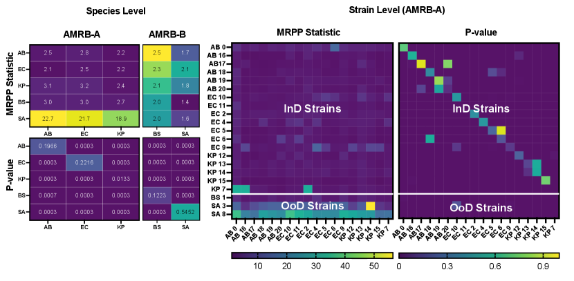
Given a bacteria classifier that maps inputs into classes (species), and a new sample (strain) potentially outside the species, we apply our method to check whether that sample resembles one of species. By following the same steps as our toy example, we formulated two hypothesis tests, one at strain-level labels (i.e., comparing strains to strains) and another at species-level labels (i.e., comparing species to species). Figure 4 shows our findings. Here, we find that a majority of strain-to-strain tests yield statistically significant differences, except when both samples belong to the same species.
6 Conclusion
In this paper, we present an approach to quantify whether a sample is out-of-distribution to a deep neural network. We formulate our method as a two-sample hypothesis test performed on an ensemble of OoD metrics. In particular, we use the Multi-Response Permutation Procedure (MRPP) statistic to quantify the dissimilarity of OoD metrics across two groups, and then recompute this statistic across random permutations of group assignments to determine the significance of the true observation. The null distribution obtained in this manner, provides an interpretable basis for decision-making. We validate our method on a toy problem created using MNIST and CIFAR10 datasets, and a domain problem of detecting an unseen bacteria species for a trained classifier.
The proposed method can be used on any trained model, given that OoD metrics can be extracted from it. Yet, some OoD metrics are limited to certain model architectures, or require access to a set of anchor points for their computation (e.g. KNN metrics). Having a validation dataset would provide a source of anchor points to compute such OoD metrics. While we use the MRPP statistic in our method, one could use any function of form (e.g., Linear Regression + AUC) as the test statistic. However, the form of group difference measured would change with the statistic being used. Moreover, for the datasets we used, a mini-batch of samples and permutations were sufficient to observe a stable behavior. However, the optimal sample size and permutations may vary depending on the data and domain.
References
- [1] Ahmad, A., Hettiarachchi, R., Khezri, A., Singh Ahluwalia, B., Wadduwage, D.N., Ahmad, R.: Highly sensitive quantitative phase microscopy and deep learning aided with whole genome sequencing for rapid detection of infection and antimicrobial resistance. Frontiers in Microbiology 14, 1154620 (2023)
- [2] Hendrycks, D., Carlini, N., Schulman, J., Steinhardt, J.: Unsolved problems in ml safety. arXiv preprint arXiv:2109.13916 (2021)
- [3] Kim, G., Ahn, D., Kang, M., Park, J., Ryu, D., Jo, Y., Song, J., Ryu, J.S., Choi, G., Chung, H.J., et al.: Rapid label-free identification of pathogenic bacteria species from a minute quantity exploiting three-dimensional quantitative phase imaging and artificial neural network. bioRxiv p. 596486 (2019)
- [4] Li, Y., Di, J., Wang, K., Wang, S., Zhao, J.: Classification of cell morphology with quantitative phase microscopy and machine learning. Optics Express 28(16), 23916–23927 (2020)
- [5] Liang, S., Li, Y., Srikant, R.: Enhancing the reliability of out-of-distribution image detection in neural networks. arXiv preprint arXiv:1706.02690 (2017)
- [6] Mielke, P.W., Berry, K.J.: Permutation methods: a distance function approach. Springer (2007)
- [7] Nalisnick, E., Matsukawa, A., Teh, Y.W., Lakshminarayanan, B.: Detecting out-of-distribution inputs to deep generative models using typicality. arXiv preprint arXiv:1906.02994 (2019)
- [8] Radhakrishnan, A., Yang, K., Belkin, M., Uhler, C.: Memorization in overparameterized autoencoders. arXiv preprint arXiv:1810.10333 (2018)
- [9] Ren, J., Liu, P.J., Fertig, E., Snoek, J., Poplin, R., Depristo, M., Dillon, J., Lakshminarayanan, B.: Likelihood ratios for out-of-distribution detection. Advances in neural information processing systems 32 (2019)
- [10] Rudin, C.: Stop explaining black box machine learning models for high stakes decisions and use interpretable models instead. Nature machine intelligence 1(5), 206–215 (2019)
- [11] Sensoy, M., Kaplan, L., Kandemir, M.: Evidential deep learning to quantify classification uncertainty. Advances in neural information processing systems 31 (2018)
- [12] Sun, Y., Ming, Y., Zhu, X., Li, Y.: Out-of-distribution detection with deep nearest neighbors. In: International Conference on Machine Learning. pp. 20827–20840. PMLR (2022)
- [13] Yang, J., Zhou, K., Li, Y., Liu, Z.: Generalized out-of-distribution detection: A survey. arXiv preprint arXiv:2110.11334 (2021)
Appendix 0.A Statistics of AMRB Dataset
The dataset used in this study consists single-cell bacteria images obtained across 21 strains as whole-slide images, and segmented into image patches. Table 2 provides some statistics on its data.
| Species | Gram | Morphology | |||
| 5 | Ab | - | Rod-Shaped | 0 | 5 |
| 2 | Bs | + | Rod-Shaped | 2 | 0 |
| 7 | Ec | - | Rod-Shaped | 2 | 5 |
| 5 | Kp | - | Rod-Shaped | 0 | 5 |
| 2 | Sa | + | Spherical | 1 | 1 |
| 21 | 5 | 2 | 2 | 5 | 16 |
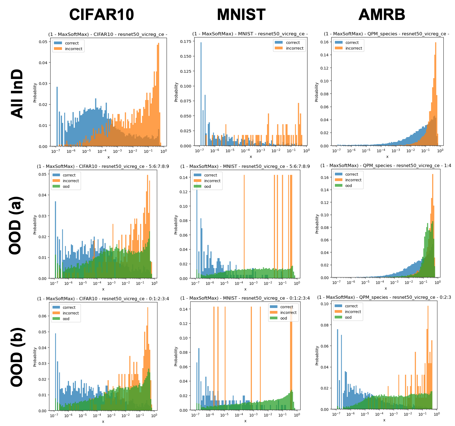
Appendix 0.B Uncertainty Quantification Measures
Here, we study the predictive uncertainty of classifiers by observing their 1-MaxSoftmax output for InD and OoD test data. For ResNet-50-EDL models, we also observe an explicit uncertainty metric , where is the logit representing the class. Fig. 5 reports our findings. In general, we observe that a well-performing classifier may perform poorly under distribution shift; i.e., when given OoD data, instead of predicting low-valued logits as expected, some logits are assigned higher values.


Appendix 0.C Separability of InD and OoD in Latent Space
Fig. 6 visualizes the separability of InD and OoD test data projected onto feature and logit spaces of different models, in 2D (UMAP). In all models, a majority of OoD data were projected close to InD data, with only a few projected further apart. Thus, it is non-trivial for a classifier trained with common loss functions to distinguish marginally OoD data from InD data.


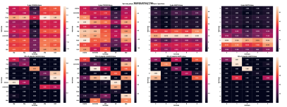
Appendix 0.D Hypothesis Testing using Model Ensembles
Here, we run hypothesis tests using combined OOD metrics from 3 model architectures (Classifier, AutoEncoder, Hybrid).

Appendix 0.E Alternative Test Statistics to MRPP
Here, we run hypothesis tests using different statistics than MRPP. In particular, we use (a) AUC and (b) Mean Difference as alternative statistics.