Identification and Mitigation of a Vibrational Telescope Systematic with Application to Spitzer
Abstract
We observed Proxima Centauri with the Spitzer Space Telescope InfraRed Array Camera (IRAC) five times in 2016 and 2017 to search for transits of Proxima Centauri b. Following standard analysis procedures, we found three asymmetric, transit-like events that are now understood to be vibrational systematics. This systematic is correlated with the width of the point-response function (PRF), which we measure with rotated and non-rotated Gaussian fits with respect to the detecor array. We show that the systematic can be removed with a novel application of an adaptive elliptical-aperture photometry technique, and compare the performance of this technique with fixed and variable circular-aperture photometry, using both BiLinearly Interpolated Subpixel Sensitivity (BLISS) maps and non-binned Pixel-Level Decorrelation (PLD). With BLISS maps, elliptical photometry results in a lower standard deviation of normalized residuals, and reduced or similar correlated noise when compared to circular apertures. PLD prefers variable, circular apertures, but generally results in more correlated noise than BLISS. This vibrational effect is likely present in other telescopes and Spitzer observations, where correction could improve results. Our elliptical apertures can be applied to any photometry observations, and may be even more effective when applied to more circular PRFs than Spitzer’s.
1 INTRODUCTION
Exoplanet science has pushed the Spitzer Space Telescope (Werner et al., 2004) far beyond its initial design. Transiting and eclipsing exoplanet signals are on the order of 1% and 0.1% of their host star, respectively, far below expected performance of the InfraRed Array Camera (IRAC, Fazio et al., 2004). Soon, the James Webb Space Telescope (JWST) will provide an unprecedented combination of spectral resolution, wavelength coverage, collecting area, and stability for exoplanet science (Deming & Seager, 2017). Currently, the field is limited to 1D characterization of most planets (e.g., Kreidberg et al., 2018), 2D thermal mapping of very hot targets (de Wit et al., 2012; Majeau et al., 2012), and 3D characterization with Hubble Space Telescope data of the hottest known planets (e.g., Stevenson et al., 2014, 2017). JWST will significantly improve planetary characterization possiblities, but small and cold planets will still be a challenge. Hotter terrestrial targets, like TRAPPIST-1b (Gillon et al., 2016, 2017), will require secondary eclipses for a confident detection (Morley et al., 2017), but temperate Earth-like targets will be difficult, if not impossible (Rauer et al., 2011; Rugheimer et al., 2015; Batalha et al., 2018; Beichman & Greene, 2018). We must take advantage of every technique available if we hope to characterize these planets.
Spitzer IRAC suffers from two primary systematic effects: an easily-removed “ramp” that causes measured flux to vary with time, and an intrapixel gain variation that creates correlations between flux and target position on the detector at a subpixel level (e.g., Charbonneau et al., 2005). These effects are present in all 3.6 and 4.5 µm observations, although the ramp is sometimes weak enough to be ignored. Several independent modeling techniques, such as Gaussian-weighted maps (Ballard et al., 2010; Lewis et al., 2013), BiLinearly Interpolated Subpixel Sensitivity (BLISS, Stevenson et al., 2012), Pixel-Level Decorrelation (PLD, Deming et al., 2015), and Independent Component Analysis (Morello, 2015) have successfully removed the position-correlated noise, enabling transiting exoplanet observations with uncertainties 100 ppm and retrieving accurate planetary parameters (Ingalls et al., 2016).
A third, much less common effect creates light-curve features that resemble transiting exoplanets. This effect has been linked to activity in the “noise pixel” parameter (Mighell, 2005; Lewis et al., 2013), a measurement of the number of pixels that contribute to centering and photometry, or the size of the point-response function (PRF). Spikes in the noise pixels are known to correlate with transit-like signals, and are likely caused by high-frequency telescope oscillations of unknown origin (see irachpp.spitzer.caltech.edu/page/np_spikes). Previous studies show that PRF Gaussian-width dependent models can account for time-evolving point-source shapes (e.g., Lanotte et al., 2014; Mendonça et al., 2018; Mansfield et al., 2020), which may be related to the noise-pixel effect.
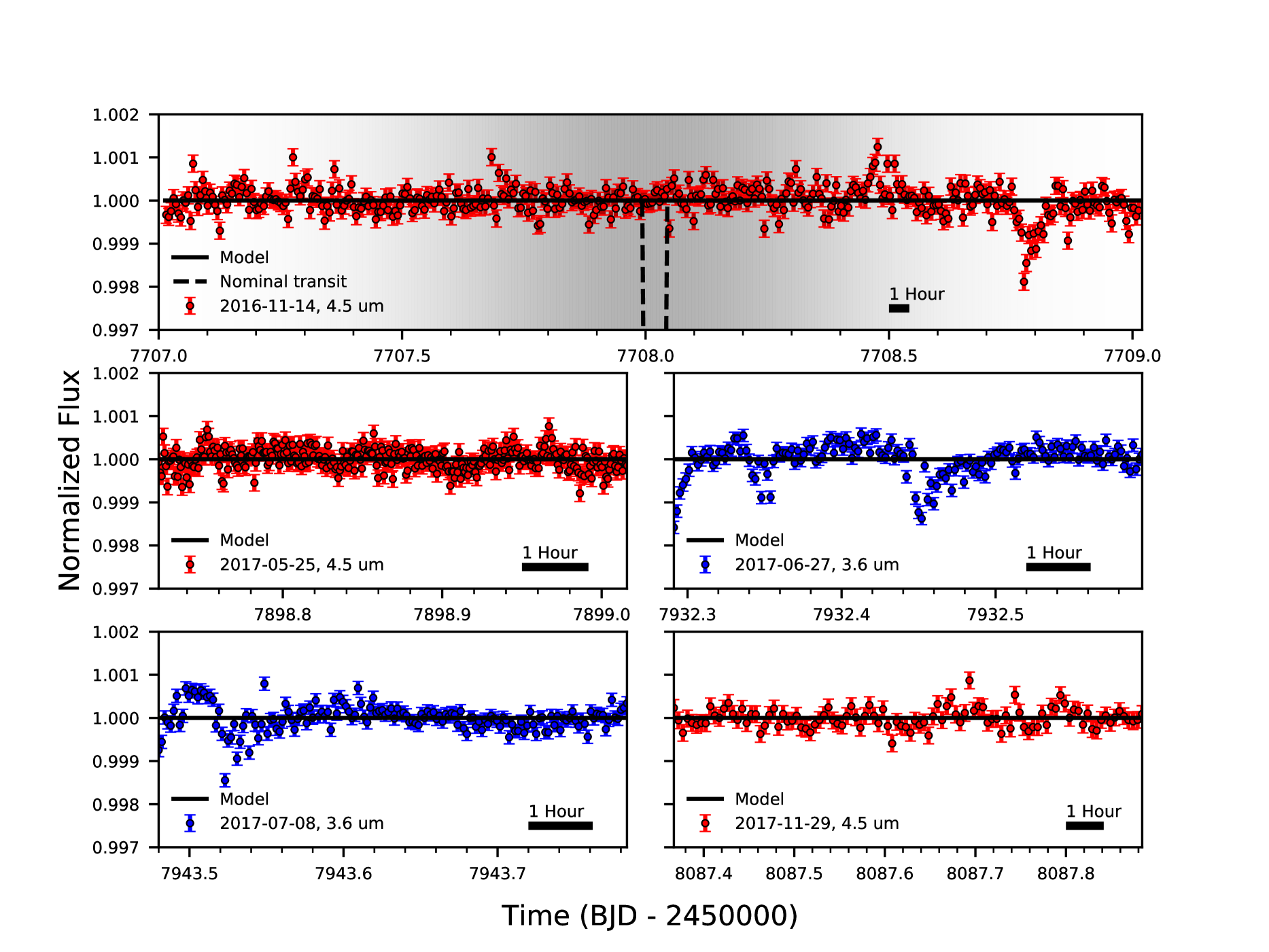
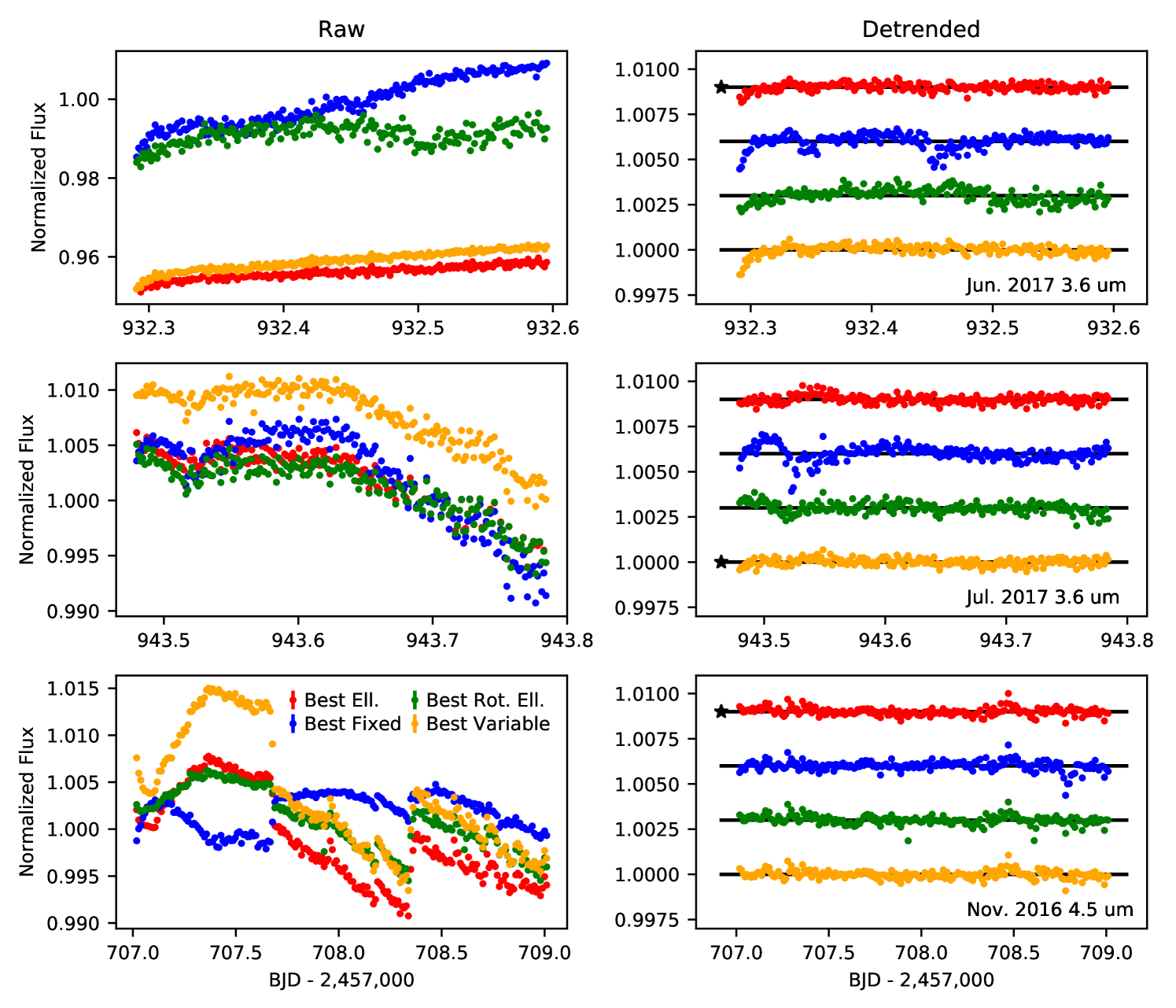
We observed Proxima Centauri (hereafter Proxima) in 2016 and 2017 with Spitzer IRAC to search for transits of the planet Proxima b (Anglada-Escudé et al., 2016). Jenkins et al. (2019), hereafter J19, presented the results from the first observation. When following standard data reduction procedures and dividing out best-fitting systematic models (with only a flat astrophysical model), these observations contain three transit-like events (see Figure 1) that resemble the asymmetric shapes created by transits of evaporating planets (e.g., Rappaport et al., 2014; Sanchis-Ojeda et al., 2015; Vanderburg et al., 2015) or comets (e.g., Rappaport et al., 2018). We now know, conclusively, that these events are localized systematic effects due to high-frequency telescopic vibration of unknown origin. When the telescope vibrates, the PRF smears along the direction of the vibration. During the vibration, fixed-radius photometry apertures spill light, resulting in lower measured flux with larger vibrational amplitudes.
In this work, we present evidence that the systematic is due to vibration, several new methods to identify when this vibrational systematic occurs, and a new aperture photometry method to correct it. The paper is organized as follows: in Section 2 we describe our observations, in Section 5 we discuss how to identify this systematic, in Section 6 we present our elliptical photometry method, in Section 8 we interpret our findings, and in Section 9 we lay out our conclusions.
2 OBSERVATIONS
=0.3in Nov. 2016 May 2017 June 2017 July 2017 Nov. 2017 Wavelength (µm ) Obs. Start (MBJDaaMBJD = Modified Barycentric Julian Date = BJD - 2450000.) Obs. Duration (hours) Frame Time (s) 0.02 0.02 0.02 0.02 0.02
We observed Proxima with the Spitzer InfraRed Array Camera, with both the 3.6 and 4.5 µm filters, for a total of hours (Table 1). The 48-hour stare bracketed the predicted transit time of Proxima b, and shorter observations occurred at times when further transits should occur, if the feature in the stare was caused by Proxima b (Anglada-Escudé et al., 2016). All observations were in subarray mode and centered on the IRAC “sweet spot”, at (-0.352″, 0.064″) and (-0.511″, 0.039″) for 3.6 µm and 4.5 µm, respectively. We bracketed each science observation with an initial 30-minute observation to minimize telescope pointing settling and a final 10-minute observation, for those who wish to generate their own dark frames, per Spitzer Science Center recommendations.
Notably, due to the brightness of the target, our observations utilized the shortest frame time, 0.02 seconds, which allows temporal resolution of high-frequency effects. To handle the large data volume from this cadence, our observations have data gaps. The 48 hour 4.5 µm stare has 17-second gaps between 64-frame subarray chunks, 24-second gaps between Astronomical Observation Requests (AORs), and minute gaps every 16 hours for data downlink and target reacquisition. Both 3.6 µm observations have 6 second gaps between subarray chunks and 14 second gaps between AORs. The shortest 4.5 µm observation has 2 – 2.5-second gaps between subarray chunks, and only one AOR. The November 2017 4.5 µm observation has the same gaps as the 48-hour stare, without the downlink and target reacquisition.
The telescope’s heater, which introduces motion on the detector in 40-minute cycles, was turned off for the duration of all five observations, following then-current Spitzer procedures for exoplanet observations. This minimizes the impact of the intrapixel systematic, allowing closer study of other effects.
3 CENTERING AND PHOTOMETRY
We use the Photometry for Orbits, Eclipses, and Transits code (POET, Stevenson et al., 2012; Blecic et al., 2013; Cubillos et al., 2013; Blecic et al., 2014; Cubillos et al., 2014; Hardy et al., 2017, e.g.,) for all analyses herein. The steps in producing light curves are bad pixel identification, determining the location of the target (centering), and measuring its brightness (photometry). We identify bad pixels by performing a twice-iterated 4 rejection on 64-frame chunks, and discard these pixels from further analysis. This work relies heavily on different centering and photometry methods, so we describe our implementations in detail.
3.1 CENTERING METHODS
We apply four centering methods: Gaussian fitting, rotated-Gaussian fitting, center-of-light, and least asymmetry (Lust et al., 2014). Our Gaussian fitting includes parameters for and position, widths in both dimensions, a height, and a constant background level. Center-of-light calculates an average position, weighted by the brightness of each pixel, much like a center-of-mass calculation. Least asymmetry computes an asymmetry value for each pixel by considering the symmetry of surrounding flux values and then fitting an inverted Gaussian to determine the point of least asymmetry. Our rotated-Gaussian fitting is described further in Section 5. Unless stated otherwise, we perform centering on a 1717 pixel box around the target. Least asymmetry uses a 99 pixel box to calculate the asymmetry of a given pixel in the 1717 centering box. We did not vary these box sizes in this analysis, and they are consistent with previous works (e.g., Cubillos et al., 2014). Frames with significant positional outliers and frames where a good centering fit could not be achieved were removed from the analysis prior to modeling.
3.2 PHOTOMETRY METHODS
Since the IRAC point-spread function (PSF) is undersampled, we bilinearly interpolate all masks and images to 5 resolution, ensuring that flux is conserved. For the Boolean masks (the IRAC-supplied bad pixel masks combined with our flagged bad pixels), any interpolated value less than one is considered a bad subpixel (i.e., any subpixel between the center of a bad pixel and a good pixel are marked as bad). We then perform aperture photometry on the interpolated, masked images, increasing all relevant length scales by the interpolation factor (aperture radius, background annulus radii, etc.), so the apertures include subpixels. We calculate the background level as a mean of the pixels in a 7 – 15-pixel annulus around the centering position, consistent with previous analyses (e.g. Blecic et al., 2013; Cubillos et al., 2013; Hardy et al., 2017).
We use three aperture photometry methods: fixed, variable (Lewis et al., 2013), and elliptical (see Section 6). Fixed photometry uses a constant-size aperture throughout a given observation. We use fixed aperture radii from 1.5 to 4.5 pixels, in steps of 0.25 pixels. Variable photometry derives aperture radii from the same 1717 box used for centering, as described by Lewis et al. (2013). Our variable-aperture radii are calculated as
| (1) |
where is a scaling factor from 0.5 – 1.5 in steps of 0.25, is an offset from -1.0 – 2.0 pixels in steps of 0.5, is the noise-pixel parameter (Mighell, 2005), defined as
| (2) |
where is the intensity at pixel , considering all pixels within the centering aperture. is 2 pixels on average and varies by 0.2 pixels throughout an observation. Calculation of should be done after background subtraction, as this significantly reduces scatter in the aperture radii and noise in the light curve.
Elliptical apertures vary in size similarly to variable apertures, but use the 1 widths of the Gaussian centering fit as the base, rather than . Then, the elliptical apertures are calculated as
| (3) |
where and are the ellipse widths in and (which vary in time), ranges from 3 – 7 in steps of 1, and again covers -1.0 – 2.0 pixels in steps of 0.5 pixels. The ellipse widths typically range from 0.5 – 0.6 pixels during an observation. See Section 6 for a more in-depth description of elliptical photometry.
Regardless of photometry method, we discard any frame which contains bad pixels within the aperture. We do not discard any additional frames due to flux variation.
We use small apertures to avoid additional noise from background pixels, but they necessitate an aperture correction to account for lost light. With fixed apertures, we rescale the final photometry based on the fraction of the interpolated PSF in the aperture. For variable and elliptical photometry, we rescale on the same principle, using an average aperture size and shape. It is possible to rescale the photometry using time-variable apertures, but this negates the correction made by the photometry methods. The interpolated PSF, provided by the Spitzer Science Center, is constant, but we suspect the true PSF stretches on short timescales, making accurate rescaling on a frame-by-frame basis impossible (see Section 6 for further discussion). Regardless, we are interested in the relative photometry, not the absolute, so whether or not we scale by a constant factor has little bearing on this work.
We choose the best centering and photometry methods by minimizing the binned- (hereafter ; Deming et al., 2015) of a best-fit light-curve model. In brief, this metric searches for model residuals that behave like white noise. White noise, measured by the standard deviation of normalized residuals (SDNR), predictably scales as , where is the number of items in each bin. Therefore, we calculate log(SDNR) vs. log() for a range of , then calculate the of a line with a slope of , anchored to the log(SDNR) of the unbinned residuals (). We repeat this process for every light curve produced by each unique combination of centering and photometry methods, and take the best fit (lowest ) as optimal. See Deming et al., 2015 and Appendix A for a complete description of the calculation.
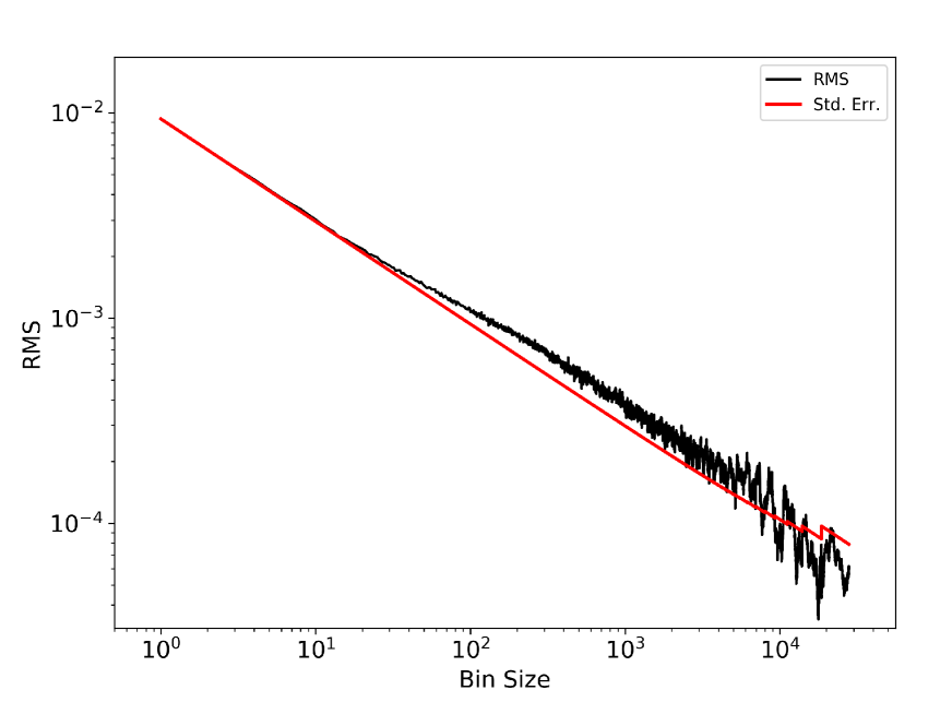
We also tested a calculation of average relative correlated noise as a metric for photometry extraction method optimization. For this metric, we calculate the expected white noise residual RMS (Pont et al., 2006; Winn et al., 2008) and measured residual RMS over all bin sizes from 1 frame to half the length of the observation, and compute the average factor between the two (see Figure 12 for an example). With BLISS models, this metric results in the same photometry methods with identical or larger aperture sizes compared to . Limiting the bin sizes to ten minutes or greater (time scales roughly relevant to eclipse, transit, and phase curve observations) did not change the result.
In addition, we experimented with a metric similar to but with the theoretical line anchored to the expected white noise unbinned residual RMS rather than the measured unbinned SDNR. Thus, this metric searches for photometric extractions that behave like white noise at all bin sizes, rather than those which only must behave similarly at large bin sizes. With BLISS, this metric selects identical extractions as (both method and aperture size). Since both these metrics led to similar results, we present only the results using .
4 LIGHT-CURVE MODELING
We modeled our light curves with both PLD and BLISS to correct the intrapixel systematic and to assess each model’s ability to address the vibrational systematic. BLISS maps correct for intrapixel sensitivity variations by gridding the detector into fine subpixels. We assign each frame to a subpixel based on the target position from centering, compute the sensitivity of each subpixel based on the average flux of all frames associated with them, once all other models (astrophysical or otherwise) have been removed, and bilinearly interpolate the sensitivity grid to find a correction factor for each frame. The generic full model formula is
| (4) |
where and are the target positions in each frame, is time, is stellar flux, is the astrophysical model, is the BLISS map, and is the time-dependent ramp. In a typical transiting exoplanet analysis, would be a combination of transits, eclipses, and phase curve variation models, but in this case, there are no modeled astrophysical variations.
PLD removes the same effect by treating the data as a weighted sum of normalized pixel values, where the weights are free parameters of the model. The model is
| (5) |
where is the number of pixels considered, are pixel weights, and are time-dependent normalized pixel values. In this work, we use the 9 brightest pixels () in our PLD models. Although it is common to bin the light curves temporally when using PLD (e.g. Deming et al., 2015; Wong et al., 2015), we do not bin the data in order to separate the models’ ability to remove correlated noise from the effects of binning (see Section 8 for further discussion). See Stevenson et al. (2012) and Deming et al. (2015) for in-depth descriptions of BLISS and PLD, respectively.
Figure 1 shows the fixed-aperture light curves, modeled with BLISS, to highlight the vibrational systematic. Aperture radii are 3.00 pixels (November 2016 4.5 µm), 2.25 pixels (May 2017 4.5 µm), 3.25 pixels (June 2017 3.6 µm), 4.50 pixels (July 2017 4.5 µm), and 2.75 pixels (November 2017 4.5 µm). The systematic is present in the November 2016 4.5 µm, June 2017 3.6 µm, and July 2017 3.6 µm light curves, so we focus on these observations going forward. While the vibration appears to be more common at 3.6 µm (2 – 3 occurrences) than at 4.5 µm (1 occurrence), possibly due to a narrower PRF, our sample size is only large enough to confirm that the vibration is not limited to one bandpass.
5 SYSTEMATIC DIAGNOSTICS
Past works used the noise pixel measurement (Equation 2) to identify activity in the PRF, and correct for it with variable-aperture photometry (e.g., Lewis et al., 2013; Deming et al., 2015; Garhart et al., 2018; Jenkins et al., 2019). Effectively, noise pixels measure the number of pixels above the background (contributing to centering and photometry). A wider (narrower) PRF should result in a larger (smaller) noise-pixel value. Since noise pixels measure an area, the radius of the photometry aperture required for the PRF is the root of the noise pixels, commonly with additional multiplicative and/or additive scaling (see Section 3.2). Thus, as the PRF size varies throughout the observation, so does the photometry aperture radius.
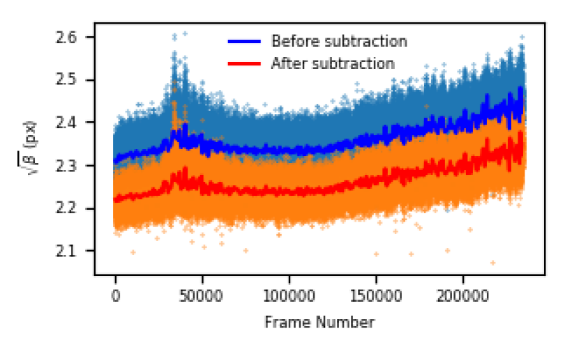
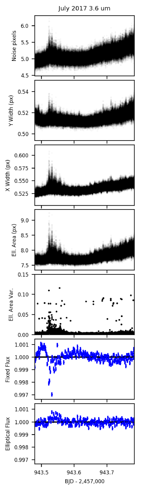
J19 found that, using common techniques, centering and photometry selection criteria selected against variable photometry apertures. We have since improved the variable-aperture photometry by calculating the aperture radii after background subtraction, which reduces uncertainty introduced by unimportant pixels. Figure 2 shows a comparison of aperture radii ( in Equation 1) in the July 3.6 µm observation when is computed before and after background subtraction. In this case, the standard deviation of decreases by %. With this improvement, variable-aperture radii are preferred over fixed-aperture radii for these observations, although they still introduce noise to the light curve due to the additional noise-pixel parameter. It is unclear if Lewis et al. (2013), who introduced variable photometry apertures, calculated noise pixels and aperture radii before or after background subtraction.
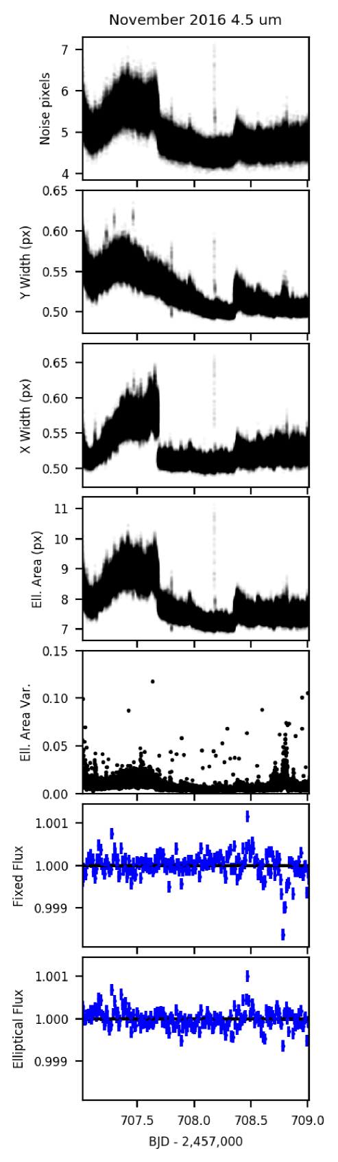
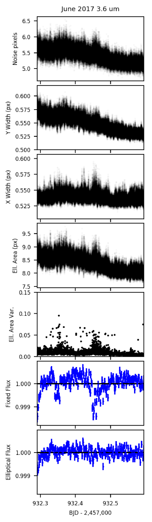
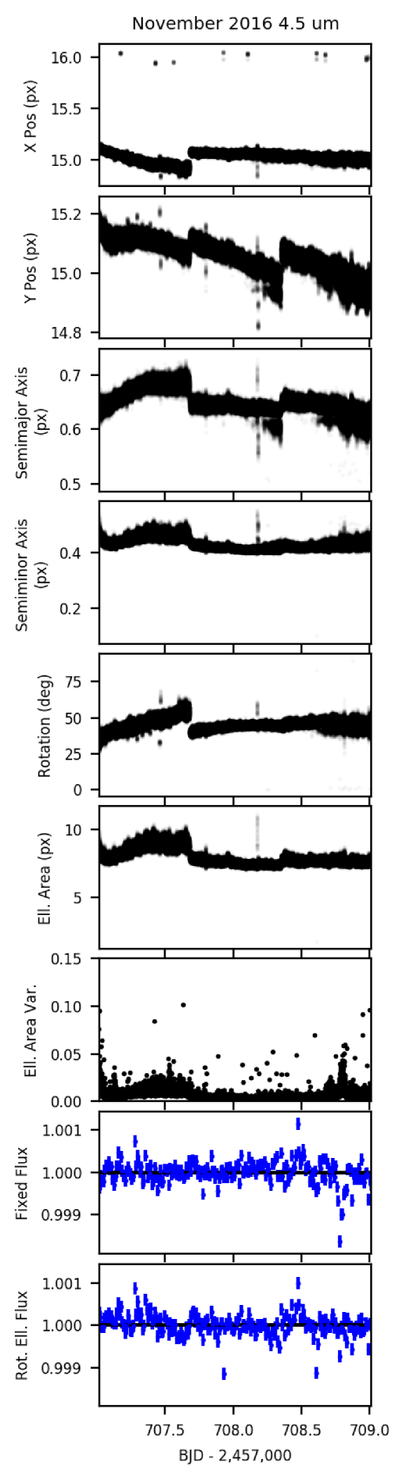
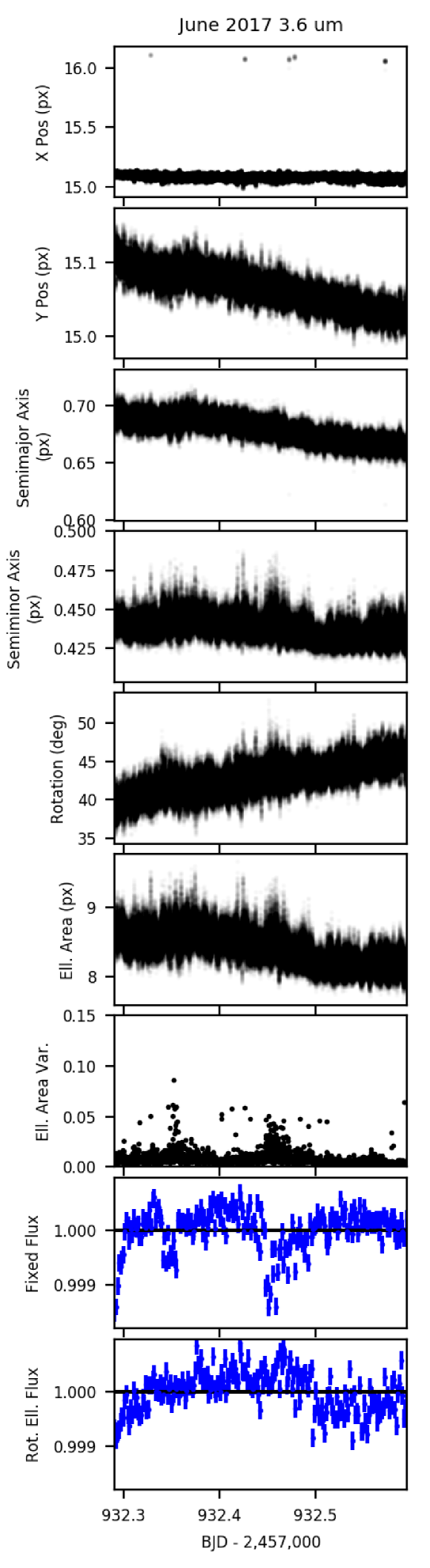
Oscillations in the telescope, if higher frequency than the exposure time, could be hidden from centering, but they would be evident in a widening of the PRF in the direction of the vibration. By fitting a Gaussian to the PRF, we determine 1 widths in and (see Figure 3, second and third rows) and notice a prominent widening in the PRF at the time of the systematic. This widening is even more evident in a measure of the 3 area of the Gaussian, which we compute as an ellipse with axes along the and directions (see Figure 3, fourth row). We also measure the variance in this elliptical area, on a 64-frame basis, to look for PRF activity (see Figure 3, fifth row).
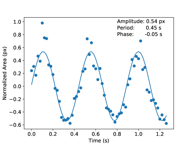
Our short exposures (0.02 seconds) allow temporal resolution of high-frequency effects. Figure 4 shows the 3 elliptical area of a single set of 64 frames during the peak of the systematic in the July 2017 3.6 µm observation. We find a clear sinusoidal pattern with a period of 0.45 seconds, evidence for telescope oscillation. Since the shape of the PRF is changing, and the photometric effect is a net loss in flux, integrating exposures by a multiple of the oscillation timescale will not correct the effect.
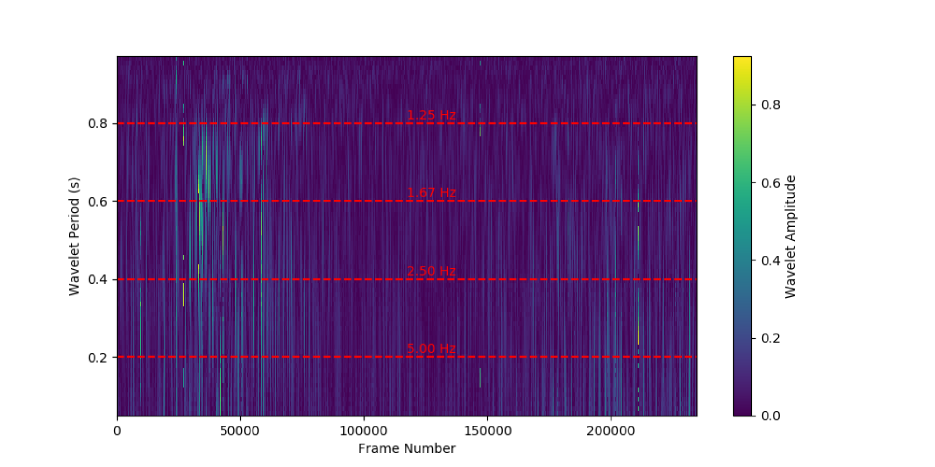
The periodicity is localized in time, so we apply a continuous Morlet wavelet transform, using the pywavelets (Lee et al., 2019) Python package (see Figure 5). Wavelet transforms assume a uniform sampling, but our observations are sets of 64 short-cadence frames separated by relatively long gaps, to work around data storage limits. This results in spurious periodicity in the wavelet transforms. Despite this limitation, a wavelet transform reveals periodic activity in the elliptical area of the PRF at the time that the systematic occurred, near frames 40,000 – 50,000. In particular, there is a cluster of stronger amplitudes at Hz, damping out to lower frequencies over the course of several thousand frames.
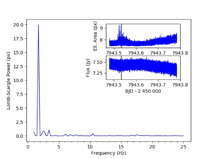
Lomb-Scargle periodograms are well-suited to finding periodicity in non-uniformly sampled data, but unlike wavelet transforms, they provide no temporal resolution of localized activity. To gain some insight into local periodicity, we use a windowed Lomb-Scargle periodogram (see Figure 6). The periodogram shows a strong peak at 2 Hz (as well as several weaker resonances), which matches the periodic behavior seen in Figure 4.
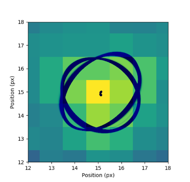
Until now, we calculated elliptical area from the and widths of the PRF. However, this measure of area is only accurate if vibrations are oriented along those axes. To more accurately measure the shape of the PRF, we rotate a Gaussian clockwise from the axis. This detaches the and widths from their respective axes, instead measuring the semimajor and semiminor axes of the ellipse. A rotated 2D Gaussian is described by
| (6) |
where
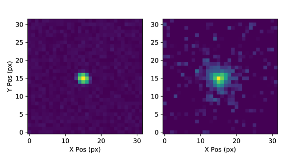
is the height of the Gaussian, is the angle of rotation clockwise from the axis, is the position of the peak, is the position of the peak, is the width along , is the width along , and is a constant background level. We fit this Gaussian function to each image using least-squares, weighted by the inverse of the Spitzer-supplied uncertainties, to determine the orientation and shape of the PRF. We tested this algorithm on both a synthetic rotated, elliptical Gaussian and an image from our observations (see Figure 7). The results are listed in Table 2. The difference in retrieved star position is small but differences in the measured PRF widths are more significant.
=-0.3in Method Background Synthetic Image Truth — — 0.600 0.500 15.000 15.000 87000 (0.524) 100.0 Std. Gaussian 0.570 0.521 — — 15.004 15.000 87135 — 101.2 Rot. Gaussian — — 0.599 0.499 15.004 15.000 87187 0.526 100.2 Spitzer Image from AOR 63273472 Std. Gaussian 0.568 0.527 — — 15.107 14.892 82175 — 32.7 Rot. Gaussian — — 0.585 0.502 15.103 14.883 84120 0.508 32.9
We applied this rotated-Gaussian centering method to the observations affected by the systematic. The results are displayed in the first seven rows of Figure 8. They match the non-rotated Gaussian fits in elliptical area and elliptical area variance. These systematic identification methods perform nearly equivalently when using the non-rotated Gaussian. However, the rotated Gaussian has implications for elliptical photometry, which is discussed in Section 6.
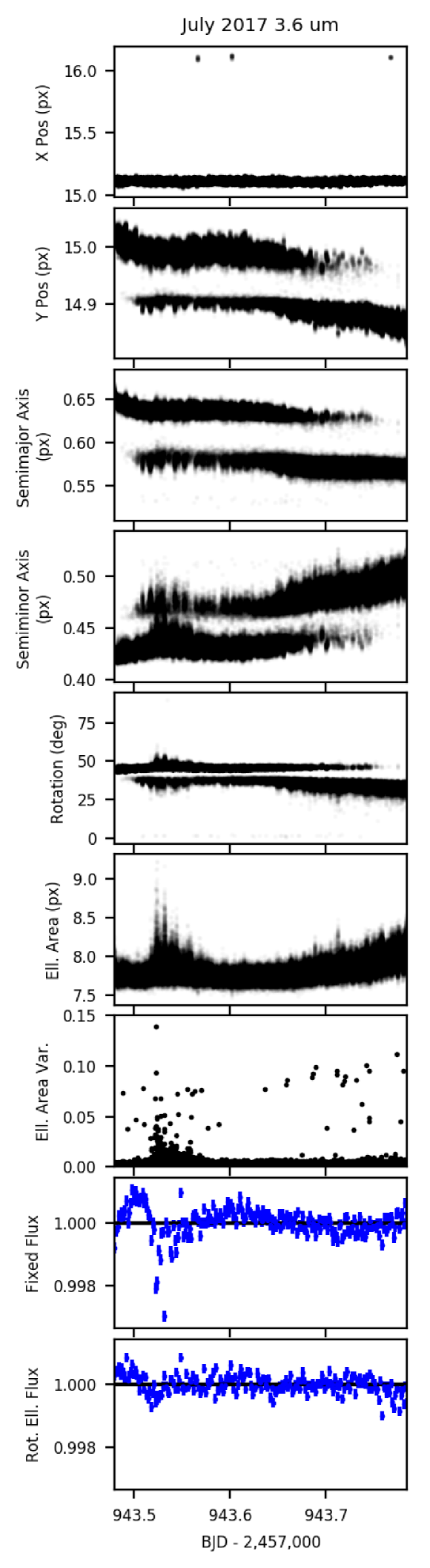
There are bimodalities in the fitted position, the axes lengths, and rotation of the ellipse when the center of the PRF passes below the center of a pixel. This behavior may be due to the asymmetry of the IRAC PRF, which has a roughly-triangular shape (e.g., the second panel of Figure 7). The ellipse is swapping between the asymmetric edges of the triangle (Figure 9). We see this behavior in the Proxima images and the synthetic images created with IRACSIM for the Spitzer data challenge (Ingalls et al., 2016), but not with simple synthetic Gaussians (Figure 7), suggesting it is a real effect of the complex PRF.
6 SYSTEMATIC REMOVAL THROUGH ELLIPTICAL PHOTOMETRY
Past works have removed this vibrational systematic prior to modeling with variable, circular apertures (e.g., Lewis et al., 2013; Deming et al., 2015; Garhart et al., 2018; Jenkins et al., 2019). These apertures adjust to avoid spilling light. However, due to their circular shape, they must either spill flux from the aperture or overcompensate in size for the elliptically-smeared PRF to capture all the important pixels; thus, they include unnecessary background noise.
Instead, we use elliptical photometry, where we use an elliptical aperture described by the fitted parameters from the non-rotated Gaussian or rotated-Gaussian centering methods described in Section 5. With rotated Gaussian centering, we apply the rotation to the elliptical aperture. Similar to using variable-aperture photometry, elliptical apertures attempt to remove the effects of PRF activity prior to modeling, but only including the most important pixels, resulting in less noise. Several elliptical photometry packages exist (e.g., Laher et al., 2012; Barbary, 2016; Merlin et al., 2019), although application has been limited to correcting atmospheric effects in ground-based observations (Bowman & Holdsworth, 2019), measuring the radial surface brightness profiles of physically elliptical galaxies (e.g., Davis et al., 1985; Djorgovski, 1985; Cornell, 1989; Ryder, 1992; McNamara & O’Connell, 1992; Hayes et al., 2005), and measuring photometry of comets that move significantly during each exposure (Miles, 2009). To our knowledge, none have used elliptical apertures to correct for vibrational effects.
Qualitatively, we find that elliptical photometry almost entirely removes the vibrational systematic from the light curve, with the non-rotated ellipses outperforming the rotated ones (see Figures 3 and 8, last rows). To assess performance quantitatively, we fit BLISS and PLD models to the three observations which include the vibrational systematic. PLD performs poorly when applied to observations longer than typical eclipses and transits (Deming et al., 2015), so, for the 48-hour observation, we only consider the final 16 hours (after the final data downlink). Many PLD implementations also bin the data (e.g., Deming et al., 2015; Wong et al., 2015; Buhler et al., 2016), which can reduce short-period correlated noise. We choose not to bin to isolate each model’s ability to address correlated noise. Table 3 lists the results: -minimized photometry aperture sizes for each combination of centering and photometry methods, as well as the (lowest in bold) and SDNR for each combination, both for BLISS and PLD fits. Figure 10 shows the -minimized BLISS light curves compared with the fixed-radius aperture light curves in Figure 1. We reduced the strength of the systematic from 0.16% to 0.06% in the November 2016 4.5 µm observation, from 0.14% to 0.06% in the June 2017 3.6 µm observation, and from 0.30% to 0.03% in July 2017 3.6 µm observation, measured by the minimum of the binned photometry presented in Figure 10.
| BLISS | PLD | ||||||
|---|---|---|---|---|---|---|---|
| Photometry | Centering | Ap. SizeaaAperture sizes for variable and elliptical photometry are listed as (see Equations 1 and 3). | SDNR | Ap. SizeaaAperture sizes for variable and elliptical photometry are listed as (see Equations 1 and 3). | SDNR | ||
| (pixels) | (ppm) | (pixels) | (ppm) | ||||
| November 2016 4.5 µm (last 16 hours of observation) | |||||||
| Fixed | Gaus. | 3.00 | 21.8 | 7630 | 3.50 | 62.1 | 8173 |
| L. Asym. | 3.00 | 22.1 | 7641 | 3.25 | 61.2 | 7909 | |
| C. of L. | 4.00 | 293.2 | 8758 | 3.50 | 61.4 | 8169 | |
| Variable | Gaus. | 0.50+1.0 | 7.7 | 7583 | 0.75+2.0 | 34.7 | 8506 |
| L. Asym. | 0.50+1.0 | 9.0 | 7475 | 0.75+2.0 | 37.0 | 8509 | |
| C. of L. | 1.50+0.5 | 200.3 | 8324 | 0.75+1.5 | 35.6 | 7932 | |
| Elliptical | Gaus. | 4.00+0.5 | 5.1 | 7438 | 3.00+2.0 | 42.5 | 8216 |
| Rot. Gaus. | 3.00+1.0 | 5.1 | 7727 | 5.00+1.5 | 60.3 | 8858 | |
| June 2017 3.6 µm | |||||||
| Fixed | Gaus. | 3.25 | 58.8 | 5511 | 3.00 | 74.2 | 5375 |
| L. Asym. | 3.75 | 124.3 | 5778 | 2.75 | 76.4 | 5286 | |
| C. of L. | 4.50 | 1440.0 | 6642 | 3.25 | 73.2 | 5490 | |
| Variable | Gaus. | 0.75+0.5 | 12.5 | 5632 | 0.75+1.0 | 36.6 | 5417 |
| L. Asym. | 1.00+0.0 | 21.0 | 5657 | 0.75+0.5 | 33.6 | 5503 | |
| C. of L. | 0.50+0.5 | 150.0 | 6627 | 0.75+0.5 | 28.8 | 5375 | |
| Elliptical | Gaus. | 4.00+0.0 | 3.1 | 5295 | 5.00-0.5 | 29.3 | 5232 |
| Rot. Gaus. | 3.00+0.0 | 7.7 | 5808 | 6.00-0.5 | 31.3 | 5332 | |
| July 2017 3.6 µm | |||||||
| Fixed | Gaus. | 4.50 | 87.8 | 5926 | 4.00 | 159.0 | 5763 |
| L. Asym. | 4.50 | 30.0 | 5889 | 4.00 | 159.3 | 5754 | |
| C. of L. | 4.50 | 1175.9 | 6295 | 4.50 | 161.9 | 5982 | |
| Variable | Gaus. | 1.50-0.5 | 2.6 | 5585 | 1.50-0.5 | 55.3 | 5582 |
| L. Asym. | 1.00+0.5 | 2.5 | 5437 | 1.00+0.5 | 56.9 | 5443 | |
| C. of L. | 0.50+0.0 | 45.3 | 8682 | 0.75+0.5 | 36.9 | 5577 | |
| Elliptical | Gaus. | 7.00-1.0 | 4.9 | 5229 | 7.00-1.0 | 71.1 | 5223 |
| Rot. Gaus. | 5.00+0.0 | 23.7 | 5225 | 7.00+0.5 | 93.2 | 5803 | |
7 COMPARISON TO GAUSSIAN-WIDTH DETRENDING
Some analyses of Spitzer IRAC data found that light-curve correlated noise could be significantly reduced by combining a BLISS map with a model dependent on the Gaussian widths of the PRF (e.g., Lanotte et al., 2014; Mendonça et al., 2018; Mansfield et al., 2020). Here we compare that approach with elliptical-aperture photometry, and test the results of combining the two methods.
For the Gaussian-width detrending, we use the following generic quadratic model:
| (7) |
where are free parameters in the light-curve model and (, ) are the widths of the Gaussian fit to the PRF of each data frame. We set . This model is included in the full light-curve model as a multiplicative factor on the right side of Equation 4.
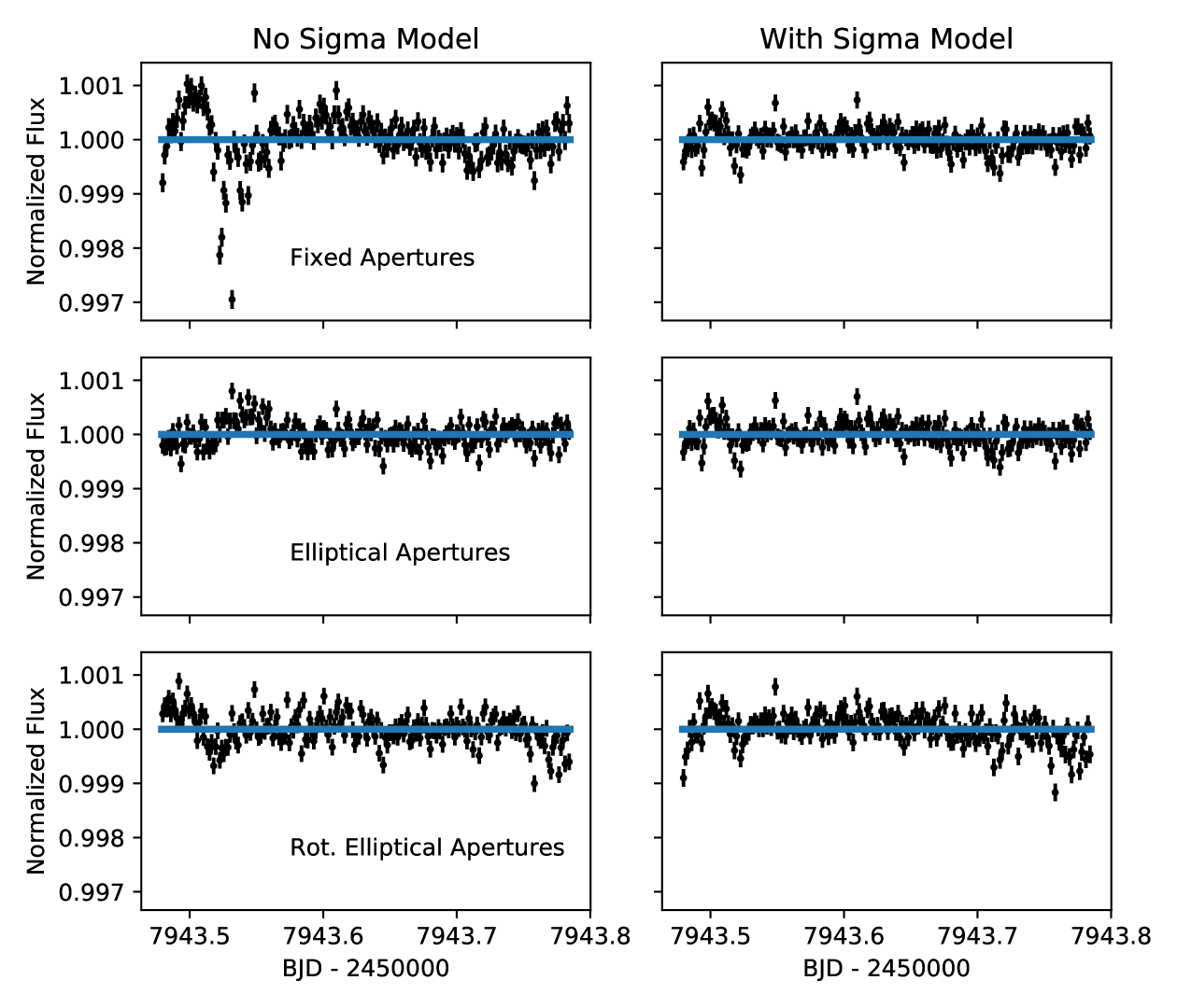
We repeat the process used in Section 6 of optimizing for the minimum in each photometry method, although we are restricted to Gaussian centering, as the Gaussian widths are an input to the light-curve model. A sample of the results is shown in Figure 11. Unsurprisingly, models that include lead to better fits (lower ) due to increased flexibility. In most cases, the noise reduction is clearly significant when applied to fixed-radius aperture photometry. However, the improvement is more marginal when the model is applied to non- and rotated elliptical apertures. For example, for the July 2017 3.6 µm observation, for non-rotated elliptical apertures improves from 4.9 to 4.8 and for rotated elliptical apertures improves from 23.7 to 19.5. In some cases including actually leads to more correlated noise because model-fitting seeks to minimize , not . For all three observations, elliptical apertures led to a lower than fixed-radius circular apertures with a Gaussian-width model.
We cannot use a statistic like the Bayesian Information Criterion (Raftery, 1995) to decide if is worth including. The -optimized photometry while including the model is different than the -optimized photometry without ; we would be comparing model fits to different data sets.
8 DISCUSSION
We draw several conclusions from the results in Table 3. First, we find elliptical photometry superior or equivalent to variable, circular apertures when using BLISS maps. The vibrational systematic is not correlated with position, especially if the vibration occurs at a period shorter than the exposure time, and thus cannot be corrected by a BLISS map. By removing the vibrational systematic with elliptical photometry, the accuracy of the BLISS map improves for the entire observation.
The PLD model is more flexible in its noise removal. It assumes that flux variations are tied to fluctuations in the pixel brightnesses. As the target moves on the detector, pixels brighten and dim. Likewise, if the PRF is smeared, pixels near the center of the target dim and pixels along the vibration axis brighten. Thus, the PLD model is able to correct for the vibrational systematic without explicit knowledge of the vibration, minimizing the advantage gained by using elliptical photometry. This is convenient, but we achieve much lower correlated noise in the BLISS models where the systematics are corrected with a physical description of their effects (see values in Table 3). We do not use binning in our application of PLD, which would reduce correlated noise, but again without explicit knowledge of the vibration. For example, when testing bin sizes of 1, 2, 4, 8, 18, 32, 64, 128, and 256 on the optimal PLD light curves from Table 3, we improve the from 34.7 to 34.3 for the November 2016 4.5 µm observation, from 28.8 to 12.0 for the June 2017 3.6 µm observation, and from 36.9 to 5.2 for the July 2017 3.6 microns observation. This suggests that temporal binning provides a significant portion of PLD’s correlated-noise correction capabilities.
The rotated ellipse is never preferred over the non-rotated case. As mentioned above, the Spitzer PRF is highly asymmetric, and slightly triangular in shape (see Figure 7, right panel), which creates a challenge when fitting a rotated ellipse. The vibration-induced elliptical shape is less prominent than the already-present asymmetry in the PRF, as evidenced by the bimodal distribution in rotation (Figure 8). We suspect that the rotated elliptical Gaussian is fitting to the sides of the triangular PRF, which creates additional noise in the resulting light curve. In particular, the bimodality creates problems for BLISS maps in two ways:
-
1.
BLISS maps rely on multiple frames at the same location to accurately calculate subpixel sensitivity. The bimodality reduces the number of frames in each sensitivity map grid cell, leading to greater uncertainty.
-
2.
The bimodality increases the size of the grid cells, which we calculate as the RMS of the point-to-point target position variation in and . This reduces the flexibility of the model, resulting in worse fits.
Rotated elliptical photometry may be useful for other telescopes that have more circular PRFs.
Since the Spitzer PRF is a complex shape, ideally we would determine flux by directly fitting the PRF, but that has proven challenging. The Spitzer PRF is underresolved, especially at shorter wavelengths, and the true PSF is not known at a high resolution, only as a map of a point source at a 55 grid of positions within a central pixel. Hence, we recommend overresolved PRFs for high-precision point-source instruments like exoplanet telescopes, or a high-resolution lab-measured PRF tested in comparison to real data with a routine to accurately bin to the native pixel level. One could also fit a shape more representative of the PRF, like a tri-lobed Gaussian with a radial scale, rotation, stretching factor, and stretching axis. However, that is beyond the scope of this work.
In general, we find that PLD is agnostic to the centering method used. In two observations, we prefer center-of-light centering, and in the third there is no strong preference for any of the methods. This would suggest that, when using PLD models, it is acceptable to only apply center-of-light centering, although we recommend always applying all methods available.
BLISS maps, on the other hand, are extremely sensitive to the centering method because 1) target position is an input to the model, and 2) we use BLISS map and grid sizes equal to the RMS of the point-to-point and target position motion, respectively. Thus, higher precision centering methods result in maps with finer structure. Compared to Gaussian and least-asymmetry centering, center-of-light centering results in high RMS of point-to-point and target position motion and, thus, poor maps, at least for 3.6 and 4.5 µm observations (Table 3). Therefore, center-of-light can be ignored with BLISS maps, although applying all analysis methods will ensure the best is chosen.
While including a Gaussian-width model can significantly reduce noise in fixed-aperture photometry, the addition of this model only slightly improves elliptical-aperture photometry. We recommend elliptical apertures over a Gaussian-width model for two reasons: 1) to reduce model complexity, and 2) to correct for correlated noise in image processing, rather than creating it with circular apertures and then modeling it out.
Finally, in nearly all cases, non-rotated elliptical photometry results in the lowest SDNR. With BLISS, elliptical photometry improves SDNR by up to 11.2% over fixed circular apertures and up to 6.0% over variable, circular apertures. With PLD, we see up to 9.4% improvement over fixed apertures and up to 6.3% improvement over variable apertures. These statistics are for the entire modeled light curve; the improvement is even more pronounced if we only consider data when the systematic is present. This suggests SDNR can be useful when optimizing photometric extraction, with the caveat that the SDNR values listed in Table 3 are for the -optimized light curves, not SDNR-optimized light curves. In our case, if we optimized solely for SDNR, we would be left with fixed-radius apertures for the November 2016 4.5 µm observation, which is clearly unsatisfactory (see Figure 1, top panel).
The optimal light curves presented here are available, in machine- and human-readable formats, in a compendium archive available at https://doi.org/10.5281/zenodo.3759914 (catalog https://doi.org/10.5281/zenodo.3759914). The compendium also includes best-fit models and correlated noise diagnostics.
9 RESULTS
We have identified a vibrational systematic in Spitzer photometry that mimics planetary or cometary transits. With our short exposure times, we were able to resolve this vibration in the size and shape of the PRF, both on sub-second timescales and with periodograms. We caution against false positive detections of planets, and recommend applying the techniques described here to identify and correct the systematic.
“Noise pixels” can occasionally identify this systematic, but they can be misleading, as noise pixel activity does not always correspond with the systematic, and can frequently be hidden in the baseline activity. Several other metrics are better suited to identifying this vibration:
-
1.
and widths from Gaussian centering, both rotated and non-rotated.
-
2.
Elliptical area of Gaussian centering, both rotated and non-rotated.
-
3.
Variance of noise pixels.
-
4.
Variance of elliptical area.
-
5.
Wavelet amplitude over a variety of frequencies.
-
6.
Lomb-Scargle periodograms of elliptical area.
For our observations, variance of the PRF area most accurately identifies the systematic. However, in most IRAC time-series observations, identification of this systematic is more challenging. The pointing wander induced by temperature fluctuation in the telescope reduces the clarity of our diagnostics.
To correct this vibrational systematic, we developed an adaptive elliptical-photometry technique. We fit an asymmetric Gaussian to the PRF to determine target position and PRF shape, and use this parameterization to create an elliptical aperture that adapts its shape to the PRF as it changes with time. We applied elliptical photometry to three observations known to include the vibrational systematic, with both BLISS and PLD models to assess relative performance. With BLISS models, elliptical photometry results in reduced correlated noise in two of our three observations, and reduced SDNR in all observations. PLD prefers variable, circular apertures over elliptical apertures, but, without binning, is less capable of removing correlated noise compared to BLISS. We also used a rotated elliptical aperture, but found that the complex shape of the Spitzer PRF created bimodalities in the orientation of the ellipse and noise in the resulting light curve. Other shapes, like a tri-lobed Gaussian, are an area of potential future study. Finally, we found that elliptical apertures outperformed traditional fixed-radius circular apertures with a Gaussian-width model.
We cannot determine the source of the vibration, though we speculate that it could be micrometeorite impacts or wear-and-tear on the telescope, such as a defect in the gyroscopes. If the source is micrometeorites, this systematic should be present in many past observations, at roughly the same rate as in our observations (four instances in 80 hours). Reanalyses with our techniques may be able to rescue data sets deemed unsalvageable, or at least improve the uncertainties on measured planetary transmission, emission, and phase curve variation. If wear-and-tear is the source of the systematic, then older observations may be unaffected, but more recent observations would still be affected. Spitzer produced high-profile exoplanet science for 16 years (e.g., Gillon et al., 2017; Kreidberg et al., 2019), much of which is done at the limit of detection. Elliptical photometry could make the difference between speculation and discovery.
Elliptical photometry is not limited to Spitzer. TESS and Kepler (and K2) are purely photometric observatories that may suffer from the same systematic. JWST also has photometric modes which will surely be used to push transiting exoplanet photometry to the smallest and coldest objects possible. Optimistically assuming that we reach the noise floor, we will need large amounts of JWST time to study these planets (e.g., Morley et al., 2017), and require the absolute best data reduction and noise removal techniques.
Spitzer (IRAC)
Appendix A Optimizing Data Sets with
In this work, we choose the optimal centering methods, photometry techniques, and photometry aperture sizes by minimizing , a measurement of residual correlated noise (Deming et al., 2015). Here we describe that calculation in detail. This calculation assesses correlated noise like a root-mean-square vs. bin size plot (see Figure 12) but in a more quantifiable way.
First, we define the standard deviation of normalized residuals (SDNR) as
| (A1) |
where is the normalized model residual for frame , is the mean of the normalized residuals, is the number of frames, and is the number of free parameters in the light-curve model. Normalized model residuals are given by
| (A2) |
where the planetless model is the best-fitting model evaluated without any planet terms (i.e., no eclipses, transits, or phase curve variation). In this particular work, there are no planets, so this is done by default.
If contains only white noise, then, when binned, SDNR should decrease (improve) by a factor of , where bin size is the number of frames over which we average. On the other hand, if there is correlated noise in , binning will not improve the SDNR as much. Thus, we define an Expected SDNR (ESDNR) as
| (A3) |
where is the number of residual points per bin (bin size), SDNRi is the SDNR with bin size , and ESDNRi is the ESDNR at bin size .
We calculate a goodness-of-fit measurement for SDNR vs. bin size compared to ESDNR, given by
| (A4) |
where is the largest integer possible such that a bin size of leaves more residual points than free parameters in the light-curve model, but does not. is the uncertainty on SDNRi, given by
| (A5) |
where is the number of residual points left after binning with bin size . In Equation A4 we bin by factors of , creating an evenly distributed number of bin sizes in log space, to avoid biasing toward data sets with less correlated noise at large bin sizes.
References
- Anglada-Escudé et al. (2016) Anglada-Escudé, G., Amado, P. J., Barnes, J., et al. 2016, Nature, 536, 437, doi: 10.1038/nature19106
- Ballard et al. (2010) Ballard, S., Charbonneau, D., Deming, D., et al. 2010, PASP, 122, 1341, doi: 10.1086/657159
- Barbary (2016) Barbary, K. 2016, The Journal of Open Source Software, 1, 58, doi: 10.21105/joss.00058
- Batalha et al. (2018) Batalha, N. E., Lewis, N. K., Line, M. R., Valenti, J., & Stevenson, K. 2018, ApJ, 856, L34, doi: 10.3847/2041-8213/aab896
- Beichman & Greene (2018) Beichman, C. A., & Greene, T. P. 2018, Observing Exoplanets with the James Webb Space Telescope (Springer International Publishing), 85, doi: 10.1007/978-3-319-55333-7_85
- Blecic et al. (2013) Blecic, J., Harrington, J., Madhusudhan, N., et al. 2013, ApJ, 779, 5, doi: 10.1088/0004-637X/779/1/5
- Blecic et al. (2014) —. 2014, ApJ, 781, 116, doi: 10.1088/0004-637X/781/2/116
- Bowman & Holdsworth (2019) Bowman, D. M., & Holdsworth, D. L. 2019, A&A, 629, A21, doi: 10.1051/0004-6361/201935640
- Buhler et al. (2016) Buhler, P. B., Knutson, H. A., Batygin, K., et al. 2016, ApJ, 821, 26, doi: 10.3847/0004-637X/821/1/26
- Charbonneau et al. (2005) Charbonneau, D., Allen, L. E., Megeath, S. T., et al. 2005, ApJ, 626, 523, doi: 10.1086/429991
- Cornell (1989) Cornell, M. E. 1989, PhD thesis, Arizona Univ., Tucson.
- Cubillos et al. (2017) Cubillos, P., Harrington, J., Loredo, T. J., et al. 2017, AJ, 153, 3, doi: 10.3847/1538-3881/153/1/3
- Cubillos et al. (2014) Cubillos, P., Harrington, J., Madhusudhan, N., et al. 2014, ApJ, 797, 42, doi: 10.1088/0004-637X/797/1/42
- Cubillos et al. (2013) —. 2013, ApJ, 768, 42, doi: 10.1088/0004-637X/768/1/42
- Davis et al. (1985) Davis, L. E., Cawson, M., Davies, R. L., & Illingworth, G. 1985, AJ, 90, 169, doi: 10.1086/113723
- de Wit et al. (2012) de Wit, J., Gillon, M., Demory, B. O., & Seager, S. 2012, A&A, 548, A128, doi: 10.1051/0004-6361/201219060
- Deming et al. (2015) Deming, D., Knutson, H., Kammer, J., et al. 2015, ApJ, 805, 132, doi: 10.1088/0004-637X/805/2/132
- Deming & Seager (2017) Deming, L. D., & Seager, S. 2017, Journal of Geophysical Research (Planets), 122, 53, doi: 10.1002/2016JE005155
- Djorgovski (1985) Djorgovski, S. B. 1985, PhD thesis, California Univ., Berkeley.
- Fazio et al. (2004) Fazio, G. G., Hora, J. L., Allen, L. E., et al. 2004, ApJS, 154, 10, doi: 10.1086/422843
- Garhart et al. (2018) Garhart, E., Deming, D., Mandell, A., Knutson, H., & Fortney, J. J. 2018, A&A, 610, A55, doi: 10.1051/0004-6361/201731637
- Gillon et al. (2016) Gillon, M., Jehin, E., Lederer, S. M., et al. 2016, Nature, 533, 221, doi: 10.1038/nature17448
- Gillon et al. (2017) Gillon, M., Triaud, A. H. M. J., Demory, B.-O., et al. 2017, Nature, 542, 456, doi: 10.1038/nature21360
- Hardy et al. (2017) Hardy, R. A., Harrington, J., Hardin, M. R., et al. 2017, ApJ, 836, 143, doi: 10.3847/1538-4357/836/1/143
- Harris et al. (2020) Harris, C. R., Jarrod Millman, K., van der Walt, S. J., et al. 2020, 585, doi: 10.1038/s41586-020-2649-2
- Hayes et al. (2005) Hayes, M., Östlin, G., Mas-Hesse, J. M., et al. 2005, A&A, 438, 71, doi: 10.1051/0004-6361:20052702
- Hunter (2007) Hunter, J. D. 2007, Computing in Science & Engineering, 9, 90, doi: 10.1109/MCSE.2007.55
- Ingalls et al. (2016) Ingalls, J. G., Krick, J. E., Carey, S. J., et al. 2016, AJ, 152, 44, doi: 10.3847/0004-6256/152/2/44
- Jenkins et al. (2019) Jenkins, J. S., Harrington, J., Challener, R. C., et al. 2019, arXiv e-prints. https://arxiv.org/abs/1905.01336
- Kreidberg et al. (2018) Kreidberg, L., Line, M. R., Thorngren, D., Morley, C. V., & Stevenson, K. B. 2018, ApJ, 858, L6, doi: 10.3847/2041-8213/aabfce
- Kreidberg et al. (2019) Kreidberg, L., Koll, D. D. B., Morley, C., et al. 2019, Nature, doi: 10.1038/s41586-019-1497-4
- Laher et al. (2012) Laher, R. R., Gorjian, V., Rebull, L. M., et al. 2012, PASP, 124, 737, doi: 10.1086/666883
- Lanotte et al. (2014) Lanotte, A. A., Gillon, M., Demory, B. O., et al. 2014, A&A, 572, A73, doi: 10.1051/0004-6361/201424373
- Lee et al. (2019) Lee, G. R., Gommers, R., Wasilewski, F., Wohlfahrt, K., & O’Leary, A. 2019, Journal of Open Source Sofware, 4, 1237, doi: 10.21105/joss.01237
- Lewis et al. (2013) Lewis, N. K., Knutson, H. A., Showman, A. P., et al. 2013, ApJ, 766, 95, doi: 10.1088/0004-637X/766/2/95
- Lust et al. (2014) Lust, N. B., Britt, D., Harrington, J., et al. 2014, PASP, 126, 1092, doi: 10.1086/679470
- Majeau et al. (2012) Majeau, C., Agol, E., & Cowan, N. B. 2012, ApJ, 747, L20, doi: 10.1088/2041-8205/747/2/L20
- Mansfield et al. (2020) Mansfield, M., Bean, J. L., Stevenson, K. B., et al. 2020, ApJ, 888, L15, doi: 10.3847/2041-8213/ab5b09
- McNamara & O’Connell (1992) McNamara, B. R., & O’Connell, R. W. 1992, ApJ, 393, 579, doi: 10.1086/171529
- Mendonça et al. (2018) Mendonça, J. M., Malik, M., Demory, B.-O., & Heng, K. 2018, AJ, 155, 150, doi: 10.3847/1538-3881/aaaebc
- Merlin et al. (2019) Merlin, E., Pilo, S., Fontana, A., et al. 2019, A&A, 622, A169, doi: 10.1051/0004-6361/201833991
- Mighell (2005) Mighell, K. J. 2005, MNRAS, 361, 861, doi: 10.1111/j.1365-2966.2005.09208.x
- Miles (2009) Miles, R. 2009, Society for Astronomical Sciences Annual Symposium, 28, 51
- Morello (2015) Morello, G. 2015, ApJ, 808, 56, doi: 10.1088/0004-637X/808/1/56
- Morley et al. (2017) Morley, C. V., Kreidberg, L., Rustamkulov, Z., Robinson, T., & Fortney, J. J. 2017, The Astrophysical Journal, 850, 121, doi: 10.3847/1538-4357/aa927b
- Pont et al. (2006) Pont, F., Zucker, S., & Queloz, D. 2006, MNRAS, 373, 231, doi: 10.1111/j.1365-2966.2006.11012.x
- Raftery (1995) Raftery, A. E. 1995, Sociological Mehodology, 25, 111
- Rappaport et al. (2014) Rappaport, S., Barclay, T., DeVore, J., et al. 2014, The Astrophysical Journal, 784, 40, doi: 10.1088/0004-637X/784/1/40
- Rappaport et al. (2018) Rappaport, S., Vanderburg, A., Jacobs, T., et al. 2018, MNRAS, 474, 1453, doi: 10.1093/mnras/stx2735
- Rauer et al. (2011) Rauer, H., Gebauer, S., Paris, P. V., et al. 2011, A&A, 529, A8, doi: 10.1051/0004-6361/201014368
- Rugheimer et al. (2015) Rugheimer, S., Kaltenegger, L., Segura, A., Linsky, J., & Mohanty, S. 2015, ApJ, 809, 57, doi: 10.1088/0004-637X/809/1/57
- Ryder (1992) Ryder, S. 1992, Australian Journal of Physics, 45, 395, doi: 10.1071/PH920395
- Sanchis-Ojeda et al. (2015) Sanchis-Ojeda, R., Rappaport, S., Pallè, E., et al. 2015, The Astrophysical Journal, 812, 112, doi: 10.1088/0004-637X/812/2/112
- Stevenson et al. (2012) Stevenson, K. B., Harrington, J., Fortney, J. J., et al. 2012, ApJ, 754, 136, doi: 10.1088/0004-637X/754/2/136
- Stevenson et al. (2014) Stevenson, K. B., Désert, J.-M., Line, M. R., et al. 2014, Science, 346, 838, doi: 10.1126/science.1256758
- Stevenson et al. (2017) Stevenson, K. B., Line, M. R., Bean, J. L., et al. 2017, AJ, 153, 68, doi: 10.3847/1538-3881/153/2/68
- Vanderburg et al. (2015) Vanderburg, A., Johnson, J. A., Rappaport, S., et al. 2015, Nature, 526, 546, doi: 10.1038/nature15527
- Virtanen et al. (2020) Virtanen, P., Gommers, R., Oliphant, T. E., et al. 2020, Nature Methods, 17, 261, doi: 10.1038/s41592-019-0686-2
- Werner et al. (2004) Werner, M. W., Roellig, T. L., Low, F. J., et al. 2004, ApJS, 154, 1, doi: 10.1086/422992
- Winn et al. (2008) Winn, J. N., Holman, M. J., Torres, G., et al. 2008, ApJ, 683, 1076, doi: 10.1086/589737
- Wong et al. (2015) Wong, I., Knutson, H. A., Lewis, N. K., et al. 2015, ApJ, 811, 122, doi: 10.1088/0004-637X/811/2/122