Identifying high-redshift GRBs with RATIR
Abstract
We present a template fitting algorithm for determining photometric redshifts, , of candidate high-redshift gamma-ray bursts (GRBs). Using afterglow photometry, obtained by the Reionization And Transients InfraRed (RATIR) camera, this algorithm accounts for the intrinsic GRB afterglow spectral energy distribution (SED), host dust extinction and the effect of neutral hydrogen (local and cosmological) along the line of sight. We present the results obtained by this algorithm and RATIR photometry of GRB 130606A, finding a range of best fit solutions for models of several host dust extinction laws (none, MW, LMC and SMC), consistent with spectroscopic measurements of the redshift of this GRB. Using simulated RATIR photometry, we find our algorithm provides precise measures of in the ranges and and can robustly determine when . Further testing highlights the required caution in cases of highly dust extincted host galaxies. These tests also show that our algorithm does not erroneously find when , thereby minimizing false negatives and allowing us to rapidly identify all potential high-redshift events.
Subject headings:
Gamma-ray bursts: general, gamma-ray bursts: specific (GRB 130606A), techniques: photometric1. Introduction
Gamma-ray bursts (GRBs) (Gehrels et al., 2009; Mészáros, 2006) are bright objects that emit across the entire electromagnetic spectrum and therefore can be seen to high-redshift (Lamb & Reichart, 2000). This allows observers to identify the locations of high-redshift, faint, host galaxy population otherwise missed by the current and future magnitude limited surveys (Tanvir et al., 2012). Such discoveries will allow us to unveil the properties of early star formation (up to ) and the epoch of reionization.
To date a number of high-redshift GRBs (all in the redshift interval ) have been identified including GRB 050904 (Totani et al., 2006), GRB 080913 (Greiner et al., 2009a), GRB 090423 (Tanvir et al., 2009) and GRB 090429B (Cucchiara et al., 2011). However, it is only in a more recent example, GRB 130606A at (Chornock et al., 2013), that high signal to noise ratio spectrum has been obtained of a high-redshift GRB afterglow. Using a method similar to that employed for quasars (Fan et al., 2006; Becker et al., 2001), the detection of Ly and Ly transmission in this spectrum allowed Chornock et al. (2013) to identify that the intergalactic medium (IGM) is mostly ionized at this redshift, and that the epoch of reionization must have occurred earlier in the history of the Universe.
Castro-Tirado et al. (2013) also present broadband photometric and spectroscopic observations of GRB 130606A, finding a lower HI column density of cm-2. Totani et al. (2013) consider a possible intervening damped Lyman- (DLA) system at as a contributor to the absorption via HI gas. Considerations of the required silicon abundance in such a DLA system lead Totani et al. (2013) to instead attribute the residuals in their host-only model to diffuse IGM along the line of sight at .
To obtain high signal-to-noise ratio spectra of potential high-redshift GRB, afterglows must first be rapidly identified. The primary method used to do so is the measurement of photometric redshifts from optical “dropout” candidates. As radiation travels through the Universe, clouds of neutral hydrogen attenuate the transmitted radiation (Madau, 1995). This effect occurs along the line of sight between source and observer, and so this attenuation encroaches into increasingly redder parts of the observed optical and near infrared (NIR) spectrum for sources (and therefore atomic hydrogen clouds) at higher redshifts.
In practice, few facilities can provide the necessary photometry to identify high-redshift candidate as most automatic, robotic telescopes use optical filters and as such are not sensitive to high-redshift GRBs. In some instances, where large aperture ground-based facilities suffer observational constraints, spectral information may not be obtained prior to the GRB afterglow fading below instrumental sensitivity limits, such as for GRB 090429B (Cucchiara et al., 2011), providing further motivation to obtain photometric redshift, , estimates for high-redshift dropout candidates. Whilst (90% likelihood range) was later obtained, additional rapid-response from GRB-dedicated NIR multiple filter instruments would have assisted in providing a measure of and allowing large aperture telescopes to begin observations at the earliest possible epoch after the initial trigger.
The variable is estimated by fitting templates to the optical and NIR spectral energy distributions (SEDs; see for example Krühler et al. 2011 and Curran et al. 2008) observed for the afterglow of the GRB, which has an intrinsic synchrotron spectrum (Granot & Sari, 2002; Sari et al., 1998). Through this template fitting method the redshift of a GRB, the host galaxy dust extinction and the optical/NIR spectral index of the GRB afterglow can be estimated. Fitting a host extinction law allows a study of the prevalence of dust in early galaxies along GRB sight lines (Zafar et al., 2011), whilst the local spectral index can be compared to that obtained in other energy ranges to determine key parameters of the underlying synchrotron spectrum (Perley et al., 2013).
To determine , Krühler et al. (2011) make extensive use of data from the Gamma-Ray Burst Optical/Near-Infrared Detector (GROND; Greiner et al. 2008). GROND simultaneously images in seven filters: g’, r’, i’, z’, J, H and KS, providing a broad optical and NIR SED. Such an SED was used to determine the for GRB 080916C (Greiner et al., 2009b) and another indicated helped identify that GRB 080913 was a high redshift event () and warranted further observations from large aperture facilities (Greiner et al., 2009a).
Another instrument capable of providing the photometric observations needed to determine is the Reionization And Transients Infra-Red (RATIR; Butler et al. 2012) camera, which is mounted on the 1.5-meter Harold L. Johnson telescope of the Observatorio Astronómico Nacional on Sierra San Pedro Mártir in Baja California, Mexico. This facility, which became fully operational in December 2012, conducts autonomous observations (Watson et al., 2012; Klein et al., 2012) of GRB triggers from the Swift satellite (Gehrels et al., 2004). Since RATIR obtains simultaneous photometry in r, i, Z, Y, J and H, it is an excellent instrument for estimating for high-redshift GRBs and as such allows us to optimize spectroscopic observations with highly oversubscribed large telescopes.
RATIR and GROND operate in similar manners, both with best responses of order a few minutes after the initial Swift trigger time (Butler et al., 2013c; Updike et al., 2010). The filters employed by both instruments are similar, but not identical. GROND has a broader spectral coverage, extending to both higher and lower wavelengths. The lower wavelength coverage aids in the identification of , although RATIR is specifically designed to target objects in the high-redshift Universe. While GROND also has a KS-band filter, extending coverage to higher redshifts, RATIR contains a Y-band filter that GROND lacks. With such functionality, RATIR is better able to provide more precise estimates of when a GRB occurs . RATIR is also 100% time dedicated to GRB follow-up. Perhaps the most important distinction between the two instruments is in their locations. RATIR is situated at latitude , while GROND is mounted on the 2.2-meter MPI/ESO telescope at La Silla Observatory, Chile, with a latitude , meaning the both form a complimentary pair of instruments routinely accessing different parts of the sky.
This work describes the development of our template fitting routine. In §2 we describe the models employed to produce the templates fitted to the RATIR optical and NIR data. In §3 we describe the Swift and RATIR observations of GRB 130606A, before in §4 presenting the results from analysis of the early epoch RATIR data. We then extensively test the capabilities of our algorithm with simulated RATIR data in §5. Finally, we present our conclusions in §6
2. Method
To measure we adopt a template fitting methodology similar to that of Krühler et al. (2011), who use combined data sets from GROND and both the Ultraviolet/Optical Telescope (UVOT; Roming et al. 2005) and X-ray Telescope (XRT; Burrows et al. 2005) on board the Swift satellite. Another similar methodology is that of Curran et al. (2008), although the algorithm we implement is significantly less computationally expensive. To this end we use models of the underlying physical spectrum of the source and the mechanisms by which this spectrum is altered before reaching an observer at Earth. These processes are dust absorption from the host galaxy, attenuation from the Intergalactic Medium (IGM) and the response of the RATIR filters to incoming photons.
Unlike Krühler et al. (2011) our algorithm does not consider UVOT photometry, as only approximately 26% of Swift GRBs having UVOT detections, compared to the 60% of bursts detected by ground-based facilities (Roming et al., 2009). Following Schady et al. (2012), we also favor the extinction laws of Pei (1992), instead of the more general “Drude” model (Liang & Li, 2009) used by Krühler et al. (2011). This was done in an attempt to limit the number of parameters being fitted as the “Drude” model has four parameters compared to the one () used in the standard Pei (1992) extinction laws.
2.1. Intrinsic GRB spectrum
The emission of GRBs is attributed to synchrotron emission (Sari et al., 1998), which produces a spectrum consisting of a series of broken power-laws. The location of the synchrotron cooling break, usually found between the optical and X-ray regimes, evolves with time in a manner determined by the nature of the circumburst medium (Granot & Sari, 2002). The passage of such a cooling break through the optical and NIR bands would manifest itself through an achromatic temporal break in the GRB light curve, which we do not observe for GRB 130606A. Due to this, and to avoid the complication of additional fitting parameters, we assume that the regime in which RATIR observes was entirely within only one of the power-law segments, thus:
| (1) |
where is flux as a function of wavelength, , is the normalization corresponding to the flux at a designated wavelength, , and is the local spectral index of the power-law. Both and are in the rest frame of the radiating outflow. Traditionally, the spectrum of a GRB is represented as a function of frequency rather that wavelength, however the expression in Equation 1 is entirely equivalent and easier to combine with the dust extinction and hydrogen absorption models detailed in §2.2 and §2.3.
2.2. Host dust absorption
Once emitted, the first external effect to act upon the GRB radiation is absorption by dust in the medium of the host galaxy along the GRB sight line. Most GRB host galaxies detected in the optical and NIR regimes exhibit low amounts of dust extinction along the GRB line of sight (Starling et al., 2007; Kann et al., 2006) with the majority of SED models for a sample covering favoring . NIR data have revealed a subset (%) of GRBs to be highly extinguished () by the dust in their host galaxy from a sample spanning (Greiner et al., 2011). Schady et al. (2012) model the extinction laws for a sample of GRB host galaxies showing an ultraviolet (UV) slope comparable to that of the Large Magellanic Clouds (LMC) but an absence of the 2175 Å “bump” in hosts with low dust extinction. Conversely, Schady et al. (2012) demonstrate that hosts of highly extinguished GRBs show clear detections of the 2175 Å bump and flatter extinction curves, thereby are more consistent with that of the MW.
To account for host galaxy dust extinction, we used the graphite-silicate dust grain models presented in Pei (1992). As the dust extinction of a GRB host galaxy along the line of sight is not known a priori, the template algorithm implements models for the MW, LMC and Small Magellanic Clouds (SMC). We also consider a case with no host dust absorption.
To calculate dust absorption as a function of wavelength, we use the empirical extinction curves presented in Table 1 of Pei (1992) and the corresponding values of , where and is the extinction in magnitudes of the -band. gives the difference in extinction between the - and -bands. Both and are defined in terms of rest-frame B and V.
We dust extinction at each wavelength given in Table 1 of Pei (1992), using Equation 2, below. We then re-sample the extinction law on to a finer grid.
| (2) |
2.3. IGM attenuation
The algorithm then calculates attenuation from the intervening IGM due to absorption from clouds of neutral hydrogen along the line of sight (Gunn & Peterson, 1965). We adopt a similar methodology to that used in the hyperz111http://webast.ast.obs-mip.fr/hyperz/ software (see also Bolzonella et al. 2000) by estimating the reduction of flux from Ly and Ly absorption using Equation 3, below, which is based on Equation 17 of Madau (1995):
| (3) |
The second line of Equation 3 states the contribution from Ly, whilst the third line totals that from Ly, Ly and Ly. Å, Å, is the coefficient of Ly absorption relative to the Ly forest contribution. , and are the coefficients for Ly, Ly and Ly, respectively.
To determine which filters require the application of , we calculate using Equation 4:
| (4) |
This ratio considers how many source counts pass through the filter both with and without IGM absorption, whilst weighting the flux at each wavelength by the filter transmission curve, . A value of indicates that there is no IGM absorption in the band, and so the flux evolves slowly across the bandpass in question. Similarly, when all flux within the filter is absorbed by neutral hydrogen and is therefore not evolving across the band. In these instances we can neglect the shape of the filter transmission curves, and therefore use the first line of Equation 5.
| (5) |
When the effects of neutral hydrogen absorption lie within a particular filter, there is a sharp transition within its wavelength coverage, , and the filter requires a more detailed treatment. In such a filter there is a fraction of wavelength coverage which experiences suppression of GRB flux. We need to calculate this fraction so we can correctly predict the total average magnitude across the filter. We therefore apply a factor of to the filter magnitude, which correctly accounts for the fraction of flux that successfully reaches the telescope and passes through the filter in question. This is shown in the second line of Equation 5.
2.4. Fitting and prior probabilities
To implement the model described we used the amoeba fitting routine within idl as well as the idl Astronomy Library (Landsman, 1993). amoeba is a robust routine that can avoid local minima in parameter space.
To avoid regions of the parameter space containing unphysical values of we imposed a prior probability distribution upon the spectral index in the optical and NIR regime. This was implemented in the manner described in §2 of Reichart (2001). As the afterglow emission is attributed to synchrotron radiation, we considered three possible regimes: (i) the optical regime lies on the same power-law segment as the X-ray regime (), (ii) there is a cooling break between the two regimes in the fast cooling regime (implying ), (iii) a cooling break in the slow cooling regime () (Granot & Sari, 2002). The cooling break occurs at the synchrotron frequency emitted by electron with a Lorentz factor that causes the cooling timescale from radiation, , to equal the dynamical time of the system, (Granot et al., 2000). In the fast cooling regime and electrons cool via radiative losses faster than the dynamical timescale. The slow cooling regime is the reverse, in which the majority of electrons are unable to cool within .
These three regimes for lead to a prior probability , given in full in Equation 6. is the known information about the parameter being fitted (in our prior this is ).
| (6) |
Schady et al. (2012) discovered that approximately 50 (25/49) of their sample of X-ray and NIR detected long GRB SEDs can be well fitted assuming , so we weighted accordingly. With no further information on whether the burst is in the fast or slow cooling regime, these two options were equally weighted to be 25% of the total distribution each.
In this instance our prior is the three expected values of already discussed. Effectively, the prior probability weights the parameter space and reduces the total viable range a parameter can take. We include realistic estimates of the Gaussian width, , for each of the distributions in and so ensure is not forced to take the exact value of one of three states discussed.
2.5. Error estimation in
The primary output of the template fitting routines is a value for . To obtain an error in this value we consider a uniform grid of values for redshift, . This grid extends over the full range of potential redshifts that can be fitted (see §5). At each point of we fit , (for the no, MW, LMC and SMC type dust models) and the normalization to the intrinsic spectrum, , using amoeba whilst holding constant. To optimize the search of the parameter space using amoeba we invoke . To do so we calculate within the fitting routine and include it as an additional term of our fit statistic, , as shown in Equation 7. The first term of Equation 7 corresponds to the standard value.
| (7) |
By calculating we force amoeba to find the best fit solution at each point of which accounts for our knowledge of . We can then find a measure of the prior weighted probability distribution, , where corresponds to the full set of parameters, directly from at each value of using Equation 8. The value of where peaks is our estimate of .
| (8) |
To provide an error estimate on we then find the narrowest range of containing 90% and 99.73% of the total weighted probability distribution. The former corresponds to the 90% confidence interval, whilst the latter would correspond to the 3 confidence interval of a Gaussian distribution. Both were obtained for all four extinction models discussed in §2.2.
3. Observations of GRB 130606A
The Burst Alert Telescope (BAT; Barthelmy et al. 2005) on board Swift triggered on GRB 130606A (Swift trigger 557589) at 21:04:39 UT on 2013 June 6th (Ukwatta et al., 2013). BAT identified prompt structure at the trigger time and later, brighter -ray emission at approximately 150 seconds after the initial trigger time.
Swift/XRT detected an uncatalogued fading X-ray source, providing a more accurate position for ground-based follow-up with narrow field instruments.
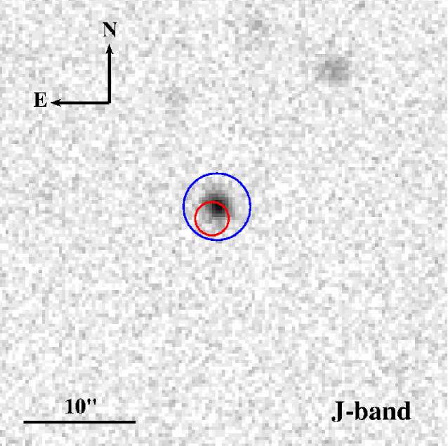
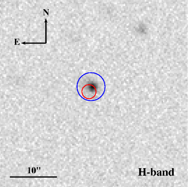
The enhanced-XRT position for GRB 130606A was found to be , with an uncertainty of (Osborne et al., 2013). This uncertainty is a radius which signifies 90% confidence. This position was calculated using the Swift/UVOT to astrometrically correct the positions of sources in the XRT field of view.
Chornock et al. (2013) observed the afterglow of GRB 130606A with both the Blue Channel spectrograph (Schmidt et al., 1989) on the Multiple Mirror Telescope (MMT) and the Gemini Multi-Object Spectrograph (GMOS; Hook et al. 2004) on the Gemini North telescope. These observations had midpoints of 7.68 and 13.1 hours after the initial BAT trigger, for the Blue Channel spectrograph and Gemini-N/GMOS respectively. From this rapid follow-up with large aperture facilities, Chornock et al. (2013) obtained high signal to noise ratio spectra allowing them to measure .
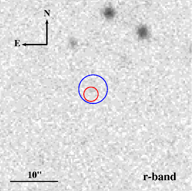
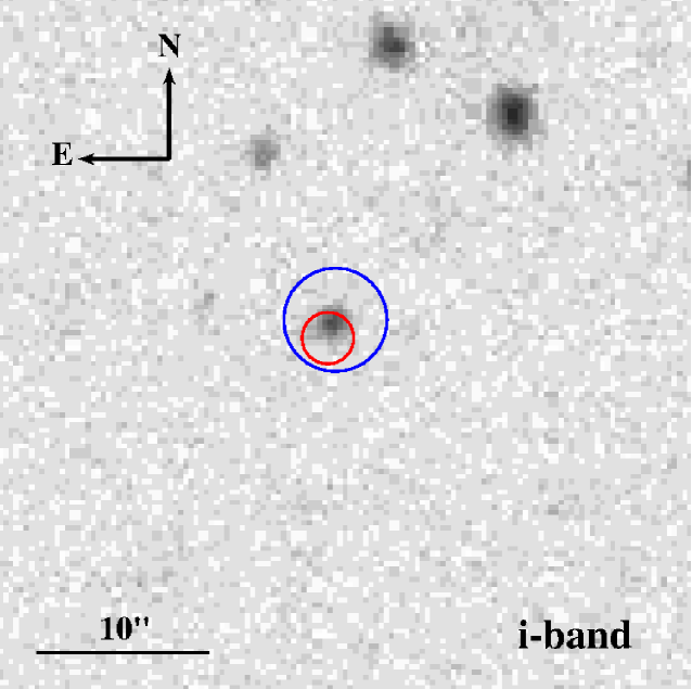
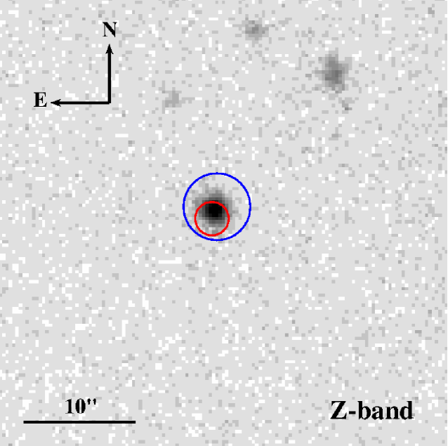
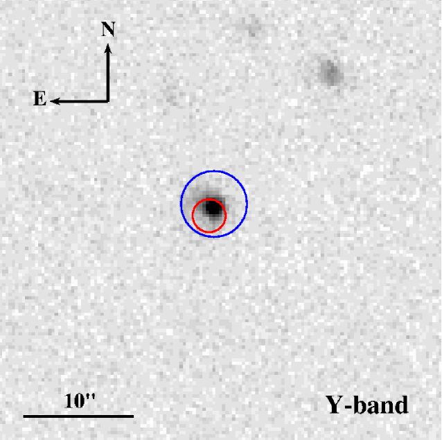
RATIR first observed the field of GRB 130606A between 7.38 and 14.19 hours after the BAT trigger. Earlier observations were precluded by the GRB occurring during daylight hours at the Observatorio Astronómico Nacional. RATIR obtained 4.42 hours of exposure in the r- and i-bands and 1.85 hours in the Z-, Y-, J- and H-bands (Butler et al., 2013b). The observations for all six photometric bands from this first night are shown in Figure 1.
A second epoch of observations were taken the following night between 31.14 and 37.86 hours after the Swift trigger (Butler et al., 2013a). With 4.96 hours of exposure time in the r- and i-bands both yielding upper limits, showing that the source had faded in the i-band. The burst remained bright enough in each of the NIR filters to allow detections in all four bands with a total exposure time of 2.07 hours. In all four filters the burst had faded by more than two magnitudes, as shown in Table 1.
The RATIR camera consists of two optical and two infrared cameras (Butler et al., 2012), allowing for simultaneous image capture in four bands ( or ). Split filters immediately above the infra-red detectors allow for near-simultaneous images in six bands by dithering the source across the infra-red detector focal plane. We employ a dither pattern that allows for sequential exposure in followed by . Dithering also allows for subtraction of the sky background and the detector dark signal at the source position. We capture 80s exposure frames in and 67s exposure frames in due to additional overhead. We apply the same image reduction pipeline – with twilight flat division and bias subtraction routines written in python and using astrometry.net (Lang et al., 2010) for image alignment and swarp (Bertin, 2010) for image co-addition – to data taken from each camera.
Photometry is calculated by running sextractor (Bertin & Arnouts, 1996) over individual science frames and mosaics over a range of apertures between 2 and 30 pixels diameter. A weighted average of the flux in this set of apertures for all stars in a given field is then used to construct an annular point-spread-function (PSF). This PSF is then fitted to the annular flux values for each source to optimize signal-to-noise for point source photometry. We perform a field-photometric calibration for the bands using the Sloan Digital Sky Survey Date Release 9 (SDSS DR9;Ahn et al. 2012). The RATIR filters have been shown to be equivalent to the SDSS filters () at the 3% level (Butler et al., in prep). We calibrate the bands relative to the Two Micron All Sky Survey (2MASS; Skrutskie et al. 2006), employing the United Kingdom Infrared Telescope (UKIRT) Wide Field Camera (WFCAM; Hodgkin et al. 2009; Casali et al. 2007) to estimate from for field stars. Photometric residuals for these bands are also approximately 3%.
| (hours) | (hours) | ||||||
|---|---|---|---|---|---|---|---|
| 7.38 | 14.19 | 24.48 0.30 | 21.80 0.06 | 19.320.02 | 19.110.02 | 18.96 0.02 | 18.64 0.02 |
| 31.14 | 37.86 | 24.06 | 23.95 | 21.500.09 | 21.410.12 | 21.160.12 | 20.780.12 |
4. Modeling GRB 130606A SED
The spectroscopic observations for GRB 130606A allow us to assess the accuracy of our template fitting routine using this burst as a test case. The standard operation of our algorithm requires input RATIR photometry and an estimation of . The former is taken from the initial RATIR GRB Coordinates Network (GCN) circular, whilst the latter is obtained from the UK Swift Science Data Centre (UKSSDC) automated analysis data products222http://www.swift.ac.uk/xrt_spectra/ (Evans et al., 2009).
The algorithm then uses a broad 1-dimensional grid in redshift () to find . This value provides a rapid and robust estimate of that aids in determining whether follow-up with large aperture facilities is warranted.
We then use 2-dimensional grids to refine our estimate of . Two such grids are used for each extinction law. The first fits and model normalization, , at fixed points in parameter space over the range . By determining the region of this parameter space with the smallest total , we then produce a second grid which focuses on the best fit solution with a higher resolution in both and .
In practice, the results from the finer, 2-dimensional grid provide a more precise estimate of . However, when coordinating follow-up from large aperture facilities, those produced from the 1-dimensional grid provide sufficiently robust estimates such that further observations can be requested at the earliest possible epoch after the initial Swift/BAT trigger.
For GRB 130606A we used RATIR photometry obtained between 7.38 and 7.79 hours after the Swift/BAT trigger time (Butler et al., 2013b). As the RATIR image reduction pipeline runs on data as it is available from the instrument, it was already possible at this epoch to identify GRB 130606A as an r-band dropout candidate. We also obtained from the UKSSDC.
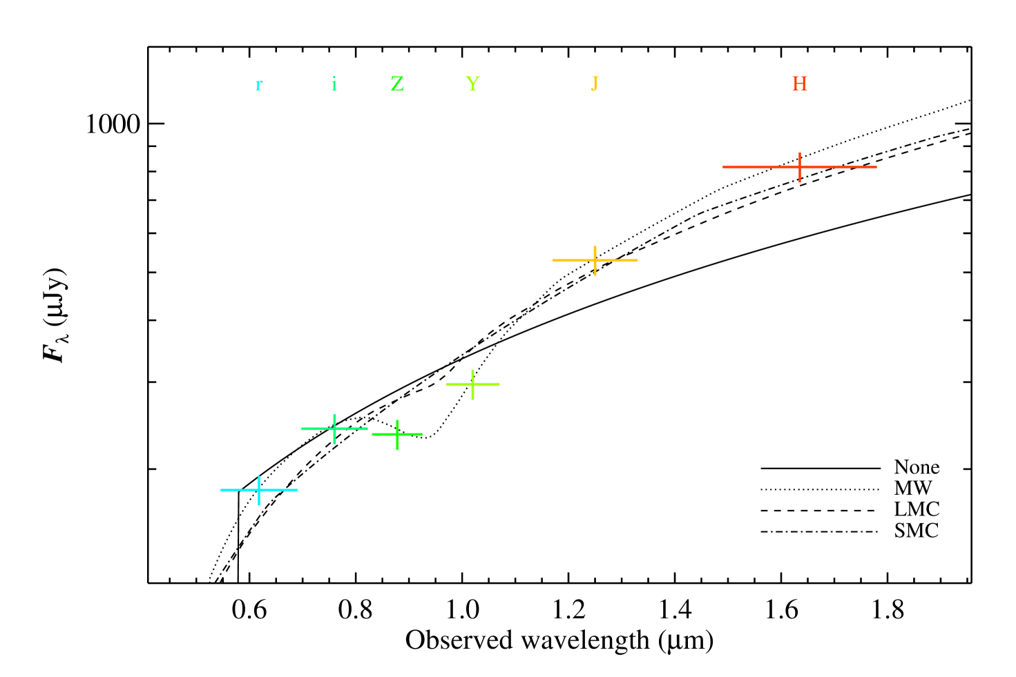
The best fit for each of the four extinction laws, the three standard templates from Pei (1992) and a fit where we assumed no host extinction, are detailed in Table 2. The corresponding templates are plotted with the RATIR photometry in Figure 2. It is important to note that we only include dust extinction from the host galaxy. For GRB 130606A, there is a possibility of an intervening system, with its own unknown dust content (Totani et al., 2013). If present, , meaning that we would be unable to distinguish between the dust in the host and any potential dust in the DLA. Even should the dust content of the DLA be high, our value of remains robust due to the small difference in redshift better then host galaxy and DLA.
| Extinction | ||||
|---|---|---|---|---|
| None | 5.97 | 0.99 | 0.00 | 2.62/3 |
| MW | 5.62 | 0.41 | 1.48 | 2.71/2 |
| LMC | 5.87 | 0.43 | 0.25 | 4.48/2 |
| SMC | 5.90 | 0.42 | 0.13 | 3.59/2 |
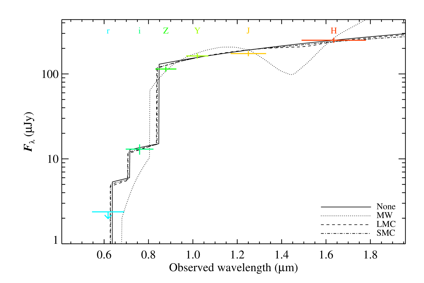
Table 2 suggests that either the MW or no-dust solution best represents the data. Visual inspection of Figure 2 suggests the LMC and SMC models are of at least comparable quality, however, the magnitude compared to that measured by RATIR is an average across the wavelength coverage of each filter. For the LMC and SMC templates, the average values across the - and -bands are more discrepant than those of the MW or no dust models. When using a MW type extinction law, a large quantity of dust is favored, with . Consequently, for the MW template is reduced, as a large quantity of dust contributes to the strong suppression of intrinsic GRB flux in the - and -bands.
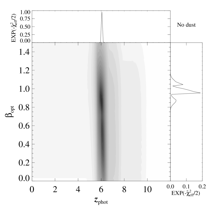
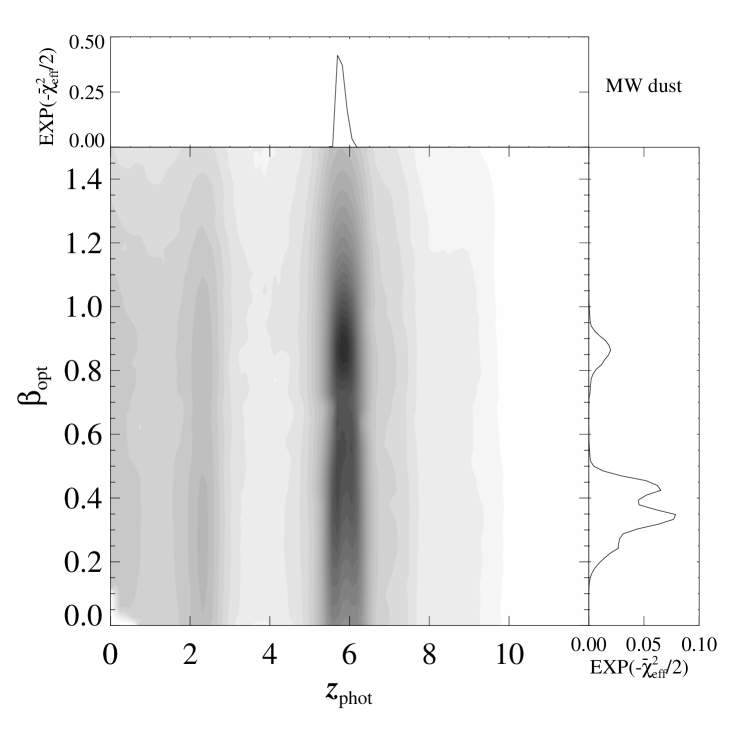
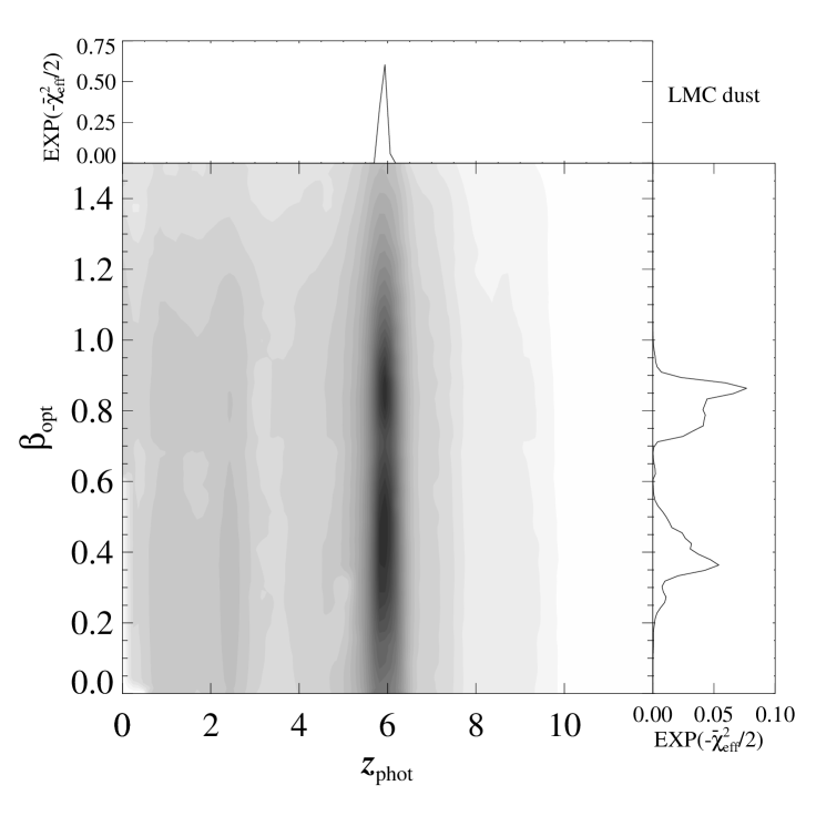

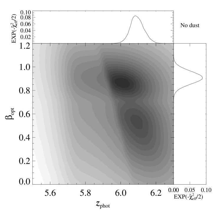
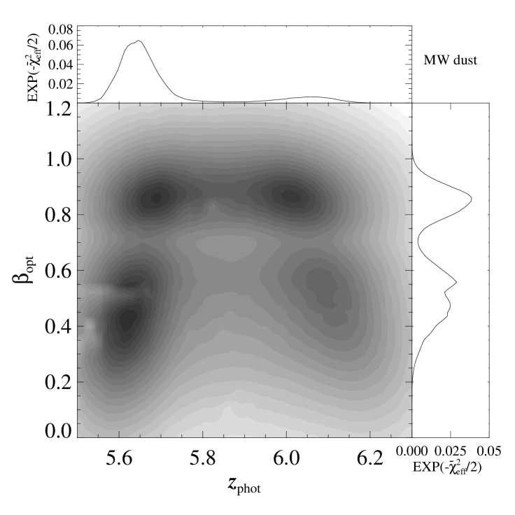
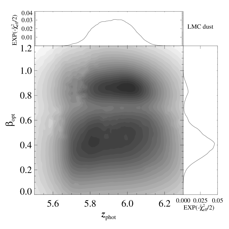
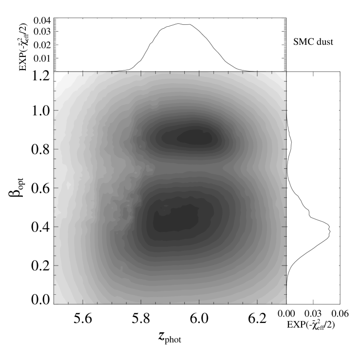
Figure 3, which contains the probability maps over all allowed ranges of , shows the best fit solutions are located in a narrow redshift range at for all four extinction laws. The finer resolution probability maps in Figure 4 allow more detailed structure to be discerned. In the no dust model there are two regions of the parameter space where the prior weighted probability is maximized. The details of the local maximum of each are in Table 3. The best found solution has and corresponds to . This is in good agreement with the cruder estimate made using the 1-dimensional grid in redshift, which is for an SED with no dust extinction (see Table 2).
The LMC and SMC probability maps in Figure 4 contain similar structure. The first solution is at , as found when . With the inclusion of a non-zero this solution is more extended in the axis. This is because at marginally lower redshifts a higher allows absorption from the IGM to contribute to the flux deficit seen at shorter wavelengths. This elongation in the axis is more pronounced in the lower solution seen for both the LMC and SMC extinction laws. Some values of do not exactly coincide with the expected values resulting from a cooling break. These result from an enhancement in the prior probability distribution between and where the slow and fast cooling break solutions overlap.
As with the extinction law, the is the better of the two alternative solutions, and indeed a fitted value of is retrieved for both the LMC and SMC extinction laws.
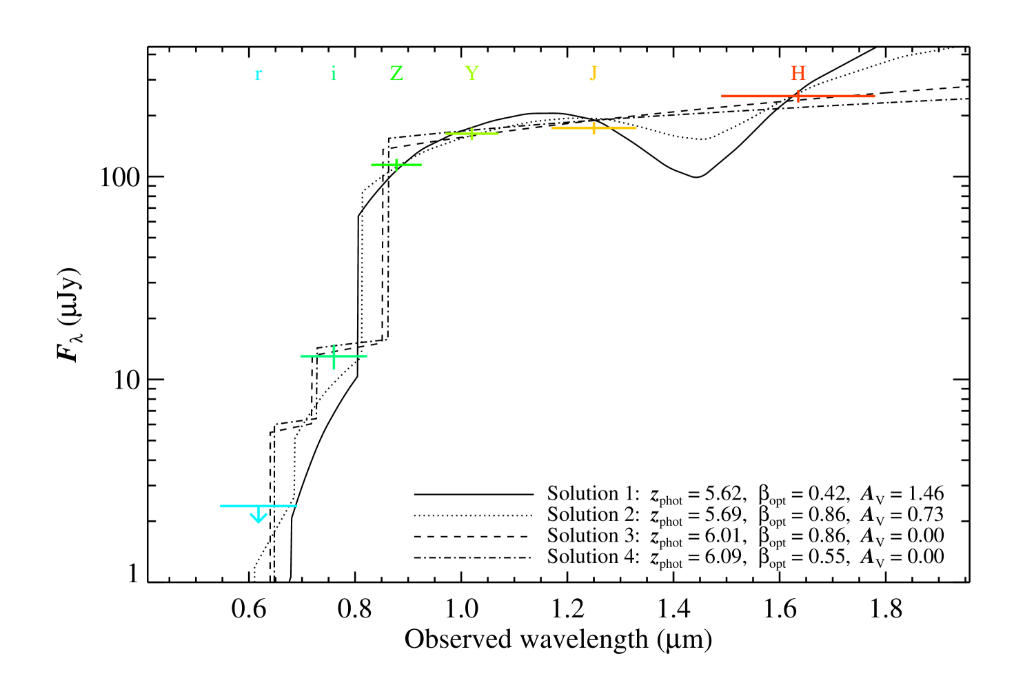
The top right panel of Figure 4 shows the same parameter space using the MW extinction law. In this instance there are four local maxima in the prior weighted probability map. The template SED for each is shown in Figure 5. The two higher solutions are equivalent to those found when . There are two additional solutions, however, at lower redshift. It is the shape of the MW extinction law that allows for these two solutions, as the 2175 Å bump can contribute to the suppression of low wavelength emission. Even with the contribution from this feature, the required is high, with the solution requiring and the lower solution requiring .
An additional point to note is the selection of the best fit from the four possible MW solutions. Table 3 shows that is lowest for solution 2 (, , ), however, when weighting by the prior probability distribution, the effective , as defined in Equation 7, is lower for solution 1 (, , ). When comparing the multiple solutions for each extinction law to the obtained spectroscopic redshift of Chornock et al. (2013), we find a solution with is most consistent with the reported value of in all cases.
As an independent test to determine which of the dust extinction laws best represents the data, we used the generic three component extinction law measured in Massa & Fitzpatrick (1986) and Fitzpatrick & Massa (1990, 1988, 1986). Applying the prior probability distribution detailed in Reichart (2001) yielded a fit where , , and . Low dust extinction disfavors solutions 1 and 2 found using a MW type extinction law (see Table 3), which both had the most discrepant values of when compared to as reported in Chornock et al. (2013).
| Extinction | Solution | ||||
|---|---|---|---|---|---|
| None | 1 | 6.01 | 0.86 | 0.00 | 2.55/3 |
| None | 2 | 6.09 | 0.55 | 0.00 | 5.24/3 |
| MW | 1 | 5.62 | 0.42 | 1.46 | 2.58/2 |
| MW | 2 | 5.69 | 0.86 | 0.73 | 2.24/2 |
| MW | 3 | 6.01 | 0.86 | 0.00 | 2.56/2 |
| MW | 4 | 6.09 | 0.55 | 0.00 | 5.30/2 |
| LMC | 1 | 6.01 | 0.86 | 0.00 | 2.55/2 |
| LMC | 2 | 5.82 | 0.44 | 0.30 | 4.00/2 |
| SMC | 1 | 6.00 | 0.86 | 0.00 | 2.58/2 |
| SMC | 2 | 5.93 | 0.45 | 0.12 | 3.43/2 |
5. Further tests of the algorithm with simulated RATIR data
We constructed simulated data to be processed with our algorithm in order to test the regions of the parameter space in which robust values of could be recovered from RATIR photometry. Specifically, we wanted to establish the range of GRB redshifts for which we could estimate , demonstrate whether the algorithm could correctly recognize the input extinction law and consider the effects of a high amount of dust extinction.
5.1. The range of
The first tests conducted were simple, with simulated input parameters , and . was chosen as it corresponded to the peak of the Swift distribution of (obtained from the on-line repository at the UKSSDC, see Evans et al. 2007). In this instance we have assumed that the optical and X-ray parts of the spectrum lie on the same power-law slope, such that . While our simulated source does not have dust extinction, we did allow for the fitting routine to determine a value for . Figure 6 shows the fitted values of compared to .
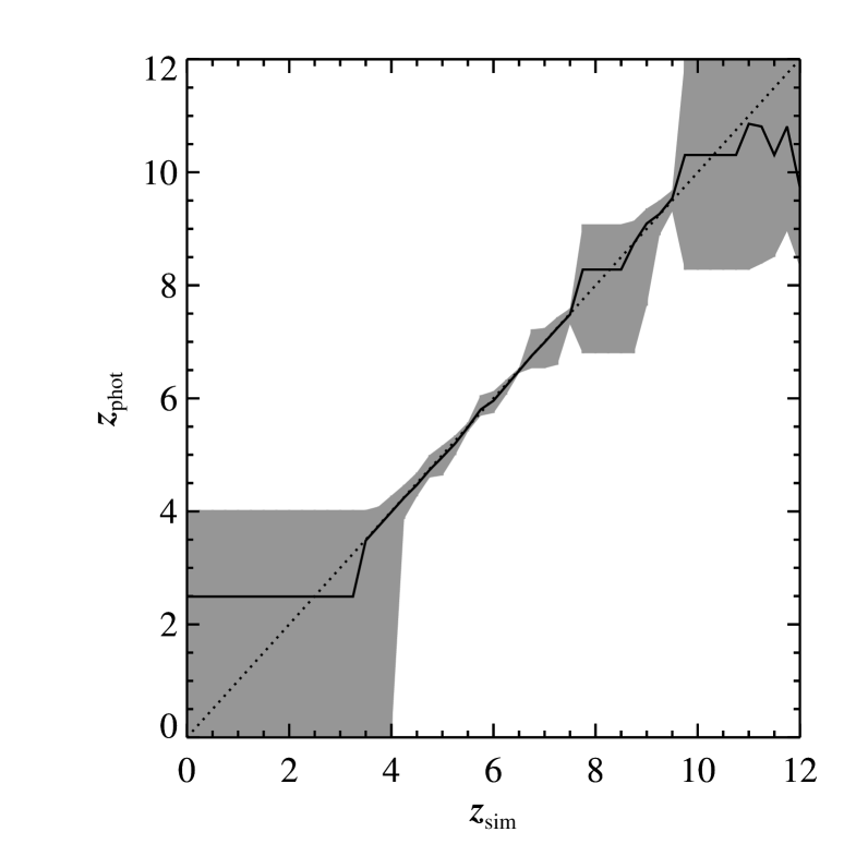
Figure 6 demonstrates some clear limitations of our algorithm when applied to RATIR data. First is the inability to measure . This is physically motivated by the observed wavelength of Ly. At , the observed wavelength of Ly is 6000 Å, placing it within the lower end of the spectral coverage of the RATIR r-band. The gray region 3 error region shows that the algorithm cannot discern the precise value of , however the lack of an r-band dropout rules out solutions where . Similar analyses can be conducted using GROND data sets, which routinely take simultaneous images in seven filters. Using the g’-band, GROND is able to determine down to (Krühler et al., 2011).
The second limit is in the . This is due to the dropout feature lying between the RATIR Y- and J-bands. In these instances, the fitting algorithm tends towards a single value of . All templates where is such that the SED features from neutral hydrogen absorption occur between bands result in an otherwise identical set of fitted parameters. This results in fits which are of identical statistical merit across a range of . To calculate the fitting routine takes an average of this range of , rather than simply taking the value of that normally corresponds to a unique best fit.
Despite not having a precise value for when the dropout occurs between the Y- and J-bands, our algorithm does still indicate that it lies between the two bands, and thus robustly confirms it is of a high redshift. Such an effect is also present when the dropout occurs between the lower wavelength filters, however, the gap in wavelength coverage is smaller and so the corresponding ranges of in which this occurs are narrower.
By comparison, GROND does not include a Y-band filter, leaving a large gap in spectral coverage between the z’- and J-bands. Indeed, Krühler et al. (2011) also encounter a similar effect to that experienced when using our fitting algorithm at . From simulations of a comparable nature to those presented here, Krühler et al. (2011) conclude that the uncertainty in their estimate of rises from at to at . The 3 confidence region for as derived from RATIR photometry similarly rises from at to at . However, this increase occurs largely when . Thus, while both RATIR and GROND can robustly infer when a GRB has , only RATIR can provide precise measurements when .
Once we found that the fitting algorithm could not recover the correct value of . Aside from the dropout feature once more falling between two photometric bands, a single photometric detection in the H-band is insufficient for the number of fitted parameters in our model.
5.2. Identifying an extinction law
In cases where the dust content is high, knowing the type of extinction law can provide valuable information regarding the circumburst medium around the GRB. Thus we tested the ability of our algorithm to distinguish between the three Pei (1992) extinction laws. To optimize the effects of the simulated dust, we chose a redshift, . This value places the 2175 Å bump at the midpoint between the RATIR - and -bands allowing the SED to most clearly define the shape of the bump. We simulated RATIR photometry at with both and , using the three Pei (1992) extinction laws, in turn.
As our algorithm is designed for use on early-time GRB photometry, to enable rapid spectroscopic follow-up, we simulated the intrinsic GRB spectra to be bright, as might be expected during the first night of RATIR observations. Each of the simulated RATIR magnitudes required a realistic error, representative of those typically reported by RATIR at these epochs, so we assigned an error of to each of simulated magnitudes. In some cases this error may prove to be conservative, with RATIR capable of measuring magnitudes to accuracies of within the first 12 hours after the initial Swift trigger (Littlejohns et al., 2013).
With simulated RATIR photometry in hand, we then used our fitting algorithm, which uses templates including all three extinction laws (and an model), to find the most representative SED for the data. Table 4 shows the full set of results obtained when fitting these simulated data.
| Input Dust | Fitted Dust | |||||
|---|---|---|---|---|---|---|
| MW | 0.25 | None | 0.00 | 3.65 | 1.11 | 12.14/3 |
| MW | 0.25 | MW | 0.24 | 3.36 | 1.02 | 2.26/2 |
| MW | 0.25 | LMC | 0.16 | 3.29 | 1.01 | 7.89/2 |
| MW | 0.25 | SMC | 1.00 | 0.06 | 0.53 | 6.57/2 |
| MW | 0.50 | None | 0.00 | 3.76 | 1.14 | 40.10/3 |
| MW | 0.50 | MW | 0.49 | 3.32 | 1.01 | 0.17/2 |
| MW | 0.50 | LMC | 0.29 | 3.35 | 1.02 | 19.28/2 |
| MW | 0.50 | SMC | 0.78 | 0.16 | 1.01 | 19.23/2 |
| LMC | 0.25 | None | 0.00 | 3.99 | 1.21 | 7.77/3 |
| LMC | 0.25 | MW | 0.53 | 0.56 | 1.02 | 0.28/2 |
| LMC | 0.25 | LMC | 0.30 | 2.19 | 1.02 | 0.42/2 |
| LMC | 0.25 | SMC | 0.56 | 0.56 | 1.03 | 0.48/2 |
| LMC | 0.50 | None | 0.00 | 4.22 | 1.37 | 40.12/3 |
| LMC | 0.50 | MW | 0.96 | 1.11 | 1.02 | 1.73/2 |
| LMC | 0.50 | LMC | 0.56 | 3.30 | 1.02 | 0.58/2 |
| LMC | 0.50 | SMC | 1.47 | 0.04 | 1.02 | 1.72/2 |
| SMC | 0.25 | None | 0.00 | 4.17 | 1.48 | 14.48/3 |
| SMC | 0.25 | MW | 0.99 | 0.11 | 1.02 | 0.44/2 |
| SMC | 0.25 | LMC | 0.75 | 0.92 | 1.02 | 0.45/2 |
| SMC | 0.25 | SMC | 0.73 | 0.91 | 1.02 | 0.38/2 |
| SMC | 0.50 | None | 0.00 | 4.41 | 1.51 | 40.16/3 |
| SMC | 0.50 | MW | 1.01 | 1.51 | 1.01 | 0.98/2 |
| SMC | 0.50 | LMC | 0.96 | 1.73 | 1.01 | 0.64/2 |
| SMC | 0.50 | SMC | 0.42 | 3.73 | 1.02 | 0.15/2 |
In all instances, our algorithm found the model to be the worst fit to the simulated photometry. The value for each fit becomes larger with increased .
For 5 of the 6 test cases, we found that the template solution with the correct extinction law yielded the fit with the smallest . The margin by which this fit was better than alternative extinction laws increased notably when increasing the amount of dust from to , as expected.
From the values shown in Table 4 it is clear that the MW type extinction law is the most easily identified by our algorithm, with the MW type template SED having the lowest and the recovered value of most closely matching in both MW tests. We demonstrate the SED templates from each of the extinction laws implemented by our algorithm in Figure 7. This more robust identification is due to the larger prominence of the 2175 Å feature in comparison to the LMC and SMC extinction laws.
The prominence of a strong 2175 Å bump in the MW extinction law has an additional implication for our fitting algorithm. At , the sharp drop in flux from neutral hydrogen absorption is not covered by the RATIR SED. In the absence of large quantities of dust in the host galaxy along the GRB sight line, our algorithm cannot determine the redshift of the GRB when . However, occurring at longer wavelengths than neutral hydrogen absorption, a strong 2175 Å feature can provide constraints on the galaxy host redshift.
Table 4 demonstrates this, as the recovered value of is in good agreement with for a MW type input extinction law with . Fitting the resulting simulated photometry with a MW extinction law the 3 error bound states . Thus, in cases of strong MW type absorption, our algorithm can determine to a slightly lower limit than indicated by the results from § 5.1. This is particularly of interest as Schady et al. (2012) note that the small sample of the GRB population with strong are best fitted with a MW type extinction law.
5.3. Fitting dusty hosts
We then considered the case where the intrinsic GRB emission is highly extinguished by dust in a host galaxy at a variety of simulated redshifts. With this in mind, we adopted 0.5. Taking into consideration the capabilities of the algorithm in the case, we only considered . As with the tests to identify dust extinction we used a bright intrinsic GRB spectrum, typical of observations within the first 12 hours after the Swift/BAT trigger. Accordingly, we assumed for all bands in which we obtained detections.
Figure 8 shows the results obtained when the same extinction law was used in both the fitted template and producing the simulated photometry. In each case we plot all values where the template fitting algorithm could successfully recover a value of . We have only included plots for the MW and LMC type extinction laws, as due to the high for the SMC extinction law, the fitting algorithm was unsuccessful in producing a unique solution for most of the values of with such a large quantity of SMC type dust in the host galaxy.
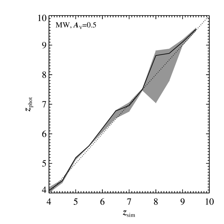
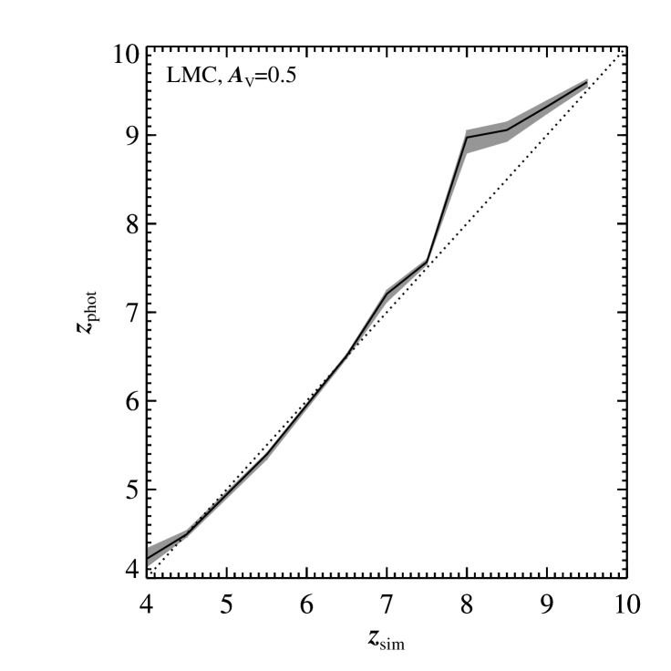
Figure 8 show the recovered values of remains consistent with prior to using the MW and LMC extinction laws. When the algorithm finds a value of that over predicts . This effect is largely due to the neutral hydrogen absorption feature falling between the RATIR - and - bands, giving large uncertainty in the precise wavelength at which it occurs. Even with the larger uncertainty in the MW extinction law simulations, we can robustly determine that in instances of a dusty GRB sight line well represented by either a MW or LMC type extinction law. Thus we retain the ability to know the GRB is of interest for further follow-up observations.
6. Conclusions
We have presented a template fitting algorithm used to determine photometric redshifts from RATIR data when a dropout candidate is present. This algorithm represents the intrinsic GRB spectrum with a physically motivated synchrotron model, includes dust extinction from the GRB host galaxy and absorption from intervening clouds of neutral hydrogen along the line of sight. Each fitted SED therefore provides estimates of , and .
Applying this algorithm to the first optical dropout candidate observed by RATIR, GRB 130606A, we successfully recover a value of (this is the range of best fit solutions), with the exact solution being dependent on the extinction law applied. This agrees well with the spectroscopic redshift obtained by Chornock et al. (2013) of . Furthermore, we demonstrate that using the prior probability distribution from Reichart (2001) for can help discern between the multiple potential solutions, as demonstrated particularly for the MW type extinction law.
We also present the typical output of the algorithm, including SEDs and probability maps of the parameter space for each extinction model. Analysis of the finely gridded probability maps, which focus on the most probably region of parameter space, shows that for an LMC or SMC type extinction law the favored model is of a host containing negligible quantities of dust. The degeneracy between several model solutions with a MW extinction law is partially lifted by using the Reichart (2001) prior probability distribution, which indicates a low value for best fits the data. With this prior probability ruling out high solutions, the best fit MW solution becomes one with negligible host dust content. With this solution, the three extinction laws all favor a near identical fit, which is consistent with a zero solution in both the obtained parameter values and fit statistic.
To ensure our algorithm is robust, we then create simulated RATIR photometry, typical of the quality expected from the first night of observations after the Swift/BAT trigger. We firstly show that when there is no dust extinction in the host galaxy, we can successfully recover using the template fitting, in the ranges and , for a variety of values. When we remain able to identify that is within this range, and is therefore a target of high interest to larger facilities.
Introducing a moderate quantity of dust extinction to our simulations allows us to draw some conclusions about the dust present in the host. MW type dust is the most easily identifiable, due to the prominent feature at 2175 Å. For weaker amounts of dust extinction it is difficult to differentiate between LMC and SMC extinction laws. However, at the two can be distinguished from one another.
An interesting result from our tests using a MW extinction law and is that the strong 2175 Å feature in the extinction law allows for a resolved value of even when neutral hydrogen absorption occurs slightly below the RATIR wavelength coverage. With a large presence of MW type dust in a host galaxy our algorithm can determine to an improved lower limit of .
We also considered simulated data containing strong host dust extinction. When simulating RATIR photometry with an SMC dust template, our algorithm was unable to resolve a solution for most values of . This is due to the large amount of suppression of low wavelength emission from the intrinsic GRB spectrum by the dust population within the host galaxy. For both the MW and LMC extinction laws precise values of were obtained for . After this point the accuracy of reduces, although we remained able to robustly state that the GRB was of high redshift. The associated 3 errors were higher with the MW extinction law due to the greater prominence of the 2175 Å feature in this type of extinction law. This allows slightly lower redshift solutions to be found where the 2175 Å bump contributes to the suppression of lower wavelength emission.
We also note that low mass stars in the Milky Way provide a population of interlopers that may occur near a Swift/XRT GRB position. To quantify the probability that such a source is present in RATIR observations we considered thick and thin disk components of the Milky Way with exponential vertical density profiles (Jurić et al., 2008). We determined the local density of M-stars within a radius of 20 pc using the Hipparcos Main Catalog (Perryman et al., 1997). This volume was chosen to simultaneously maximize completeness and the total number of sources. We cross referenced these sources with the 2MASS All-Sky Catalog of Point Sources (Cutri et al., 2003), using the cross-match service provided by CDS, Strasbourg, to obtain their J band magnitude. We found the chance probability that an M-star with J will be present in a 300 square arcsecond region centered around the Swift/XRT position is less than 2.3 %. This corresponds to one (or fewer) chance M-star in observations of approximately 43 different fields of view. Such events can be classified as non-GRB by their lack of temporal variability and the blackbody shape of the SED at low wavelengths.
Since December 2012, RATIR has observed 56 GRB fields of view, with one instance of an M-star interloper. RATIR observations of the field of GRB 131127A found a red source near the Swift/XRT position, suggesting a high-redshift candidate ideal for follow-up (Butler et al., 2013d). This source was observed at later epochs, revealing no significant evidence for fading (Butler et al., 2013e; Im et al., 2013), leading to the conclusion that this source was not a GRB.
The presented methodology is aimed specifically at identifying potential high-redshift GRBs, and providing a preliminary estimate of redshift. With in hand, the justification of triggering larger spectroscopic facilities to measure a highly resolved spectroscopic redshift is significantly higher. With the automated capabilities of RATIR it is therefore possible to request observations from such large facilities at early epochs after the initial Swift trigger time, thereby obtaining high signal-to-noise ratio spectra required to answer fundamental questions about the high-redshift Universe.
References
- Ahn et al. (2012) Ahn, C. P., Alexandroff, R., Allende Prieto, C., et al. 2012, ApJS, 203, 21
- Barthelmy et al. (2005) Barthelmy, S. D., Barbier, L. M., Cummings, J. R., et al. 2005, Space Sci. Rev., 120, 143
- Becker et al. (2001) Becker, R. H., Fan, X., White, R. L., et al. 2001, AJ, 122, 2850
- Bertin (2010) Bertin, E. 2010, SWarp: Resampling and Co-adding FITS Images Together, astrophysics Source Code Library, ascl:1010.068
- Bertin & Arnouts (1996) Bertin, E., & Arnouts, S. 1996, A&AS, 117, 393
- Bolzonella et al. (2000) Bolzonella, M., Miralles, J.-M., & Pelló, R. 2000, A&A, 363, 476
- Burrows et al. (2005) Burrows, D. N., Hill, J. E., Nousek, J. A., et al. 2005, Space Sci. Rev., 120, 165
- Butler et al. (2012) Butler, N., Klein, C., Fox, O., et al. 2012, in Society of Photo-Optical Instrumentation Engineers (SPIE) Conference Series, Vol. 8446, Society of Photo-Optical Instrumentation Engineers (SPIE) Conference Series
- Butler et al. (2013a) Butler, N., Watson, A. M., Kutyrev, A., et al. 2013a, GRB Coordinates Network, 14824, 1
- Butler et al. (2013b) —. 2013b, GRB Coordinates Network, 14799, 1
- Butler et al. (2013c) —. 2013c, GRB Coordinates Network, 14943, 1
- Butler et al. (2013d) —. 2013d, GRB Coordinates Network, 15525, 1
- Butler et al. (2013e) —. 2013e, GRB Coordinates Network, 15555, 1
- Butler et al. (in prep) Butler, N., et al. in prep
- Casali et al. (2007) Casali, M., Adamson, A., Alves de Oliveira, C., et al. 2007, A&A, 467, 777
- Castro-Tirado et al. (2013) Castro-Tirado, A. J., Sánchez-Ramírez, R., Ellison, S. L., et al. 2013, ArXiv e-prints, arXiv:1312.5631
- Chornock et al. (2013) Chornock, R., Berger, E., Fox, D. B., et al. 2013, ApJ, 774, 26
- Cucchiara et al. (2011) Cucchiara, A., Levan, A. J., Fox, D. B., et al. 2011, ApJ, 736, 7
- Curran et al. (2008) Curran, P. A., Wijers, R. A. M. J., Heemskerk, M. H. M., et al. 2008, A&A, 490, 1047
- Cutri et al. (2003) Cutri, R. M., Skrutskie, M. F., van Dyk, S., et al. 2003, 2MASS All Sky Catalog of point sources.
- Evans et al. (2007) Evans, P. A., Beardmore, A. P., Page, K. L., et al. 2007, A&A, 469, 379
- Evans et al. (2009) —. 2009, MNRAS, 397, 1177
- Fan et al. (2006) Fan, X., Strauss, M. A., Becker, R. H., et al. 2006, AJ, 132, 117
- Fitzpatrick & Massa (1986) Fitzpatrick, E. L., & Massa, D. 1986, ApJ, 307, 286
- Fitzpatrick & Massa (1988) —. 1988, ApJ, 328, 734
- Fitzpatrick & Massa (1990) —. 1990, ApJS, 72, 163
- Gehrels et al. (2009) Gehrels, N., Ramirez-Ruiz, E., & Fox, D. B. 2009, ARA&A, 47, 567
- Gehrels et al. (2004) Gehrels, N., Chincarini, G., Giommi, P., et al. 2004, ApJ, 611, 1005
- Granot et al. (2000) Granot, J., Piran, T., & Sari, R. 2000, ApJ, 534, L163
- Granot & Sari (2002) Granot, J., & Sari, R. 2002, ApJ, 568, 820
- Greiner et al. (2008) Greiner, J., Bornemann, W., Clemens, C., et al. 2008, PASP, 120, 405
- Greiner et al. (2009a) Greiner, J., Krühler, T., Fynbo, J. P. U., et al. 2009a, ApJ, 693, 1610
- Greiner et al. (2009b) Greiner, J., Clemens, C., Krühler, T., et al. 2009b, A&A, 498, 89
- Greiner et al. (2011) Greiner, J., Krühler, T., Klose, S., et al. 2011, A&A, 526, A30
- Gunn & Peterson (1965) Gunn, J. E., & Peterson, B. A. 1965, ApJ, 142, 1633
- Hodgkin et al. (2009) Hodgkin, S. T., Irwin, M. J., Hewett, P. C., & Warren, S. J. 2009, MNRAS, 394, 675
- Hook et al. (2004) Hook, I. M., Jørgensen, I., Allington-Smith, J. R., et al. 2004, PASP, 116, 425
- Im et al. (2013) Im, M., Choi, C., Lee, H., Ahn, H. N., & Pak, S. 2013, GRB Coordinates Network, 15548, 1
- Jurić et al. (2008) Jurić, M., Ivezić, Ž., Brooks, A., et al. 2008, ApJ, 673, 864
- Kann et al. (2006) Kann, D. A., Klose, S., & Zeh, A. 2006, ApJ, 641, 993
- Klein et al. (2012) Klein, C. R., Kubánek, P., Butler, N. R., et al. 2012, in Society of Photo-Optical Instrumentation Engineers (SPIE) Conference Series, Vol. 8453, Society of Photo-Optical Instrumentation Engineers (SPIE) Conference Series
- Krühler et al. (2011) Krühler, T., Schady, P., Greiner, J., et al. 2011, A&A, 526, A153
- Lamb & Reichart (2000) Lamb, D. Q., & Reichart, D. E. 2000, ApJ, 536, 1
- Landsman (1993) Landsman, W. B. 1993, in Astronomical Society of the Pacific Conference Series, Vol. 52, Astronomical Data Analysis Software and Systems II, ed. R. J. Hanisch, R. J. V. Brissenden, & J. Barnes, 246
- Lang et al. (2010) Lang, D., Hogg, D. W., Mierle, K., Blanton, M., & Roweis, S. 2010, AJ, 139, 1782
- Liang & Li (2009) Liang, S. L., & Li, A. 2009, ApJ, 690, L56
- Littlejohns et al. (2013) Littlejohns, O., Butler, N., Watson, A. M., et al. 2013, GRB Coordinates Network, 15420, 1
- Madau (1995) Madau, P. 1995, ApJ, 441, 18
- Massa & Fitzpatrick (1986) Massa, D., & Fitzpatrick, E. L. 1986, ApJS, 60, 305
- Mészáros (2006) Mészáros, P. 2006, Reports on Progress in Physics, 69, 2259
- Osborne et al. (2013) Osborne, J. P., Beardmore, A. P., Evans, P. A., & Goad, M. R. 2013, GRB Coordinates Network, 14811, 1
- Pei (1992) Pei, Y. C. 1992, ApJ, 395, 130
- Perley et al. (2013) Perley, D. A., Cenko, S. B., Corsi, A., et al. 2013, ArXiv e-prints, arXiv:1307.4401
- Perryman et al. (1997) Perryman, M. A. C., Lindegren, L., Kovalevsky, J., et al. 1997, A&A, 323, L49
- Reichart (2001) Reichart, D. E. 2001, ApJ, 553, 235
- Roming et al. (2005) Roming, P. W. A., Kennedy, T. E., Mason, K. O., et al. 2005, Space Sci. Rev., 120, 95
- Roming et al. (2009) Roming, P. W. A., Koch, T. S., Oates, S. R., et al. 2009, ApJ, 690, 163
- Sari et al. (1998) Sari, R., Piran, T., & Narayan, R. 1998, ApJ, 497, L17
- Schady et al. (2012) Schady, P., Dwelly, T., Page, M. J., et al. 2012, A&A, 537, A15
- Schmidt et al. (1989) Schmidt, G. D., Weymann, R. J., & Foltz, C. B. 1989, PASP, 101, 713
- Skrutskie et al. (2006) Skrutskie, M. F., Cutri, R. M., Stiening, R., et al. 2006, AJ, 131, 1163
- Starling et al. (2007) Starling, R. L. C., Wijers, R. A. M. J., Wiersema, K., et al. 2007, ApJ, 661, 787
- Tanvir et al. (2009) Tanvir, N. R., Fox, D. B., Levan, A. J., et al. 2009, Nature, 461, 1254
- Tanvir et al. (2012) Tanvir, N. R., Levan, A. J., Fruchter, A. S., et al. 2012, ApJ, 754, 46
- Totani et al. (2006) Totani, T., Kawai, N., Kosugi, G., et al. 2006, PASJ, 58, 485
- Totani et al. (2013) Totani, T., Aoki, K., Hattori, T., et al. 2013, ArXiv e-prints, arXiv:1312.3934
- Ukwatta et al. (2013) Ukwatta, T. N., Barthelmy, S. D., Gehrels, N., et al. 2013, GRB Coordinates Network, 14781, 1
- Updike et al. (2010) Updike, A., Nicuesa, A., Nardini, M., Kruehler, T., & Greiner, J. 2010, GRB Coordinates Network, 10874, 1
- Watson et al. (2012) Watson, A. M., Richer, M. G., Bloom, J. S., et al. 2012, in Society of Photo-Optical Instrumentation Engineers (SPIE) Conference Series, Vol. 8444, Society of Photo-Optical Instrumentation Engineers (SPIE) Conference Series
- Zafar et al. (2011) Zafar, T., Watson, D. J., Tanvir, N. R., et al. 2011, ApJ, 735, 2