Identifying Shared Decodable Concepts in the Human Brain Using Image-Language Foundation Models
Abstract
We introduce a method that takes advantage of high-quality pretrained multimodal representations to explore fine-grained semantic networks in the human brain. Previous studies have documented evidence of functional localization in the brain, with different anatomical regions preferentially activating for different types of sensory input. Many such localized structures are known, including the fusiform face area and parahippocampal place area. This raises the question of whether additional brain regions (or conjunctions of brain regions) are also specialized for other important semantic concepts. To identify such brain regions, we developed a data-driven approach to uncover visual concepts that are decodable from a massive functional magnetic resonance imaging (fMRI) dataset. Our analysis is broadly split into three sections. First, a fully connected neural network is trained to map brain responses to the outputs of an image-language foundation model, CLIP (Radford et al., 2021). Subsequently, a contrastive-learning dimensionality reduction method reveals the brain-decodable components of CLIP space. In the final section of our analysis, we localize shared decodable concepts in the brain using a voxel-masking optimization method to produce a shared decodable concept (SDC) space. The accuracy of our procedure is validated by comparing it to previous localization experiments that identify regions for faces, bodies, and places. In addition to these concepts, whose corresponding brain regions were already known, we localize novel concept representations which are shared across participants to other areas of the human brain. We also demonstrate how this method can be used to inspect fine-grained semantic networks for individual participants. We envisage that this extensible method can also be adapted to explore other questions at the intersection of AI and neuroscience.
1 Introduction
To navigate the world, individuals must learn to quickly interpret what they see. Evolution created pressure to quickly extract certain types of visual information. For example recognizing and interpreting faces is core to many of our social interactions, recognizing animate objects is key to avoiding a predator (or pursuing prey). As a byproduct, the visual system identifies a core set of concepts necessary for a successful existence in our world. But what are these core concepts, and how does the brain represent them? Seeking the answer to this question has been central to decades of neuroscience research.
Some have argued that the brain has specific areas tuned to detecting specific concepts. There is significant evidence suggesting there are areas of the brain that preferentially activate for stimuli containing faces (Kanwisher et al., 1997), places (Epstein and Kanwisher, 1998), and more recently, there have been reports of food-specific brain areas (Jain et al., 2023, Pennock et al., 2023). The controversy around these findings is driven largely by the observation that the brain areas are not “tuned” specifically for faces or places; they also respond to other visual stimuli, meaning they are not face- or place-specific (Haxby et al., 2001, Hanson and Halchenko, 2008). Thus, the key question remains unanswered: Are there dimensions of meaning recoverable from the brain’s responses to image stimuli that are consistent in 1) content, and 2) localization across participants?
In this work we take an entirely data-driven approach to uncovering dimensions of meaning within the human brain. We use the Natural Scenes Dataset (Allen et al., 2022), one of the largest and most comprehensive visual stimulus functional Magnetic Resonance Imaging (fMRI) datasets to date, and CLIP, a shared text and image embedding space (Radford et al., 2021). We present a new decoding model that produces high top-1 accuracy, predicting CLIP space from fMRI. We then use the predicted CLIP space to learn a new embedding space we call the Shared Decodable Concept (SDC) space. SDC-space:
-
1.
is trained across participants specifically to identify the dimensions of meaning that are decodable from fMRI
-
2.
has a small number of coherent concepts per dimension
-
3.
shows consistent cross-participant localization in brain-space
SDC-space allows for a data-driven mapping of concepts to brain areas, which allowed us to find several new concepts localized to specific brain areas.
The hunt for concept-specific areas of the brain has been a decades-long venture. Very early work focused on the tuning of neurons for very low level features Hubel and Wiesel (1959), followed by the discovery of brain areas preferentially activated for specific concepts and dimensions of semantic meaning (Kanwisher et al., 1997, McCandliss et al., 2003, Noppeney, 2008). These studies were largely hypothesis-driven, with stimuli chosen specifically to search for areas tuned to certain concepts.
Hypothesis-driven experimental design is a cornerstone of neuroscience research, and has contributed greatly to our current understanding of the brain. However, recently some have argued for a more data-driven naturalistic approach to neuroscience (Matusz et al., 2019, Hamilton and Huth, 2020, Khosla et al., 2022). Our work differs from previous data-driven approaches in that we perform dimensionality reduction in CLIP embedding space. For contrast, other work does the dimensionality reduction directly in fMRI voxel space, often for a single ROI. By using voxels from multiple ROIs, our method makes use of all of the information decodable from cortex. In addition, or SDC space has dimensions that are highly interpretable. This is in stark contrast to other methods, like Principal Components Analysis (PCA) where the different dimensions often lack interpretability. Our SDC space also leverages connections between the true and predicted CLIP space, which is not possible with typical PCA-style analyses.
A data-driven approach has the potential to uncover brain areas tuned to concepts that we might not otherwise have considered, as well as to expand our understanding of the specificity of certain brain areas beyond narrow visual concept classes. What follows is a framework for uncovering such visual concepts that suggests multiple new avenues for future hypothesis-driven research.
2 Decoding CLIP-Space from Brain Images
To identify shared decodable concepts in the brain, we require a mapping from brain space to a suitable representational space. In this section we describe the pieces necessary for creating this mapping: a multimodal image-language embedding model (CLIP), a brain imaging dataset (NSD), and our method to map from per-image brain responses to their associated multimodal embeddings. We consider two models in this section, and verify that our proposed neural network decoder outperforms a regression-based linear model.
2.1 Data
fMRI Data
The natural scenes dataset (NSD) is a massive fMRI dataset acquired to study the underpinnings of natural human vision. Eight participants were presented with 30,000 images (10,000 unique images over 3 repetitions) from the Common Objects in Context (COCO) naturalistic image dataset (Lin et al., 2014). A set of 1,000 shared images were shown to all participants, while the other 9,000 images were unique to each participant. Single-trial beta weights were derived from the fMRI time series using the GLMSingle toolbox (Prince et al., 2022). This method fits numerous haemodynamic response functions (HRFs) to each voxel, as well as an optimised denoising technique and voxelwise fractional ridge regression, specifically optimised for single-trial fMRI acquisition paradigms. Some participants did not complete all sessions, and three sessions were held out by the NSD team for the Algonauts challenge. Further details can be found in Allen et al. (2022).
Representational Space for Visual Stimuli
To generate representations for each stimulus image, we use a model trained on over 400 million text-image pairs with the contrastive language-image pretraining objective (CLIP (Radford et al., 2021)). The CLIP model consists of a text-encoder and image-encoder that are jointly trained to maximize the cosine similarity of corresponding text and image embeddings in a shared low-dimensional space. We use the 32-bit Transformer model (ViT-B/32) implementation of CLIP to create 512-dimensional representations for each of the stimulus images used in the NSD experiment. We train our decoder to map from fMRI responses during image viewing to the associated CLIP vector for that same image.
2.2 Data Preparation
Data Split
We randomly split the per-image brain responses and CLIP embeddings into training , validation , and test folds. The validation and test folds were each chosen to have exactly 1,000 images. Some participants in the NSD did not complete all scanning sessions and only viewed certain images once or twice. We assign these images to the training set. Of the shared 1,000 images, 413 were shown three times to every participant across the sessions released by NSD. These 413 images appear in each participant’s testing fold.
Voxel Selection
The noise ceiling is often used to identify the voxels that most reliably respond to visual stimuli. The NSD fMRI data comes with voxelwise noise ceiling estimates, but they are calculated using the full dataset. These estimates can be used to extract a subset of voxels for decoding analyses, but this takes into account voxel sensitivity to images we later want to tune and test on, and is a form of double-dipping (Kriegeskorte et al., 2009). We therefore re-calculated the per-voxel noise ceiling estimates specifically on the designated training data only. Voxels with noise ceiling estimates above variance explainable by the stimulus were used as inputs to the decoding model, resulting in 10k-30k voxel subsets per participant (see Supplementary Info for exact per-participant voxel dimensions).
2.3 Decoding Methodology
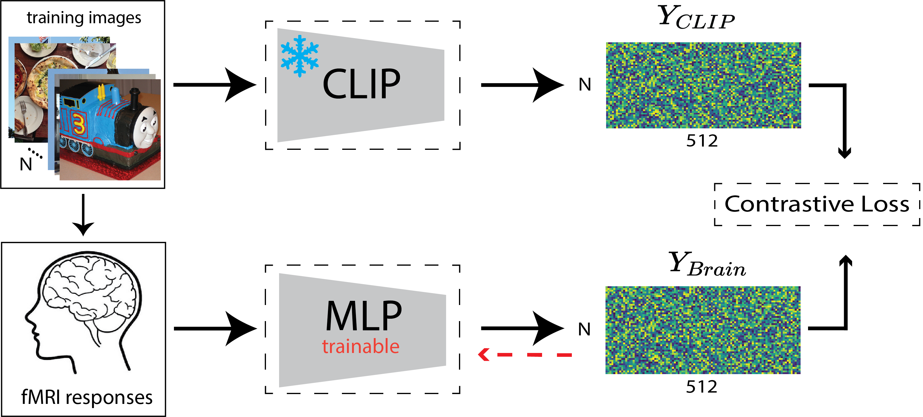
Decoding Model
The decoding model is trained to map a vector of brain responses to the CLIP embeddings of the corresponding stimulus images . Here is the number of training instances, and is the number of voxels. An illustration of the decoding procedure is given in 1(a). We define to be a multi-layer perceptron (MLP) with a single hidden layer of size 5,000, following by a leaky ReLU activation (slope=0.01). The model is trained for 12 epochs (approximately 1,500 iterations) with the Adam optimizer and a batch size of 128. The learning rate is initialized to and decreased by a factor of 10 after epochs 3, 6, and 9. We train the brain decoder using the the InfoNCE loss function (van den Oord et al., 2018), which is defined as:
| (1) |
In the original CLIP setting, and both represent image and language embeddings, where the loss is minimized when these embeddings have a high similarity for the same images (positive class) and low similarity otherwise. In our implementation, we replace the language embeddings with the brain responses to images. We set in our implementation. We compare our model to a baseline ridge regression model trained on the same data. We used grid search to select the best ridge regularization parameter using the validation data.
Evaluation
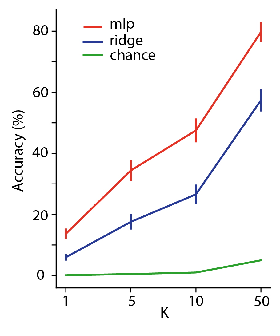
We evaluate our models using top-k accuracy, which is computed by sorting in ascending order all true representations by their cosine distance to a predicted representation . Top-k Accuracy is the percentage of instances for which the true representation is amongst the top-k items in the sorted list. Chance top-k accuracy is where is the number of held-out data points used for evaluation. Figure 1(b) shows the results of this evaluation. The MLP model outperforms ridge regression across all values of , motivating the need for this more complex model.
Recall that our end goal is to identify shared decodable concepts (SDC) in the brain. Our methodology for this task relies on the predicted CLIP vectors, and so an accurate deocoding model is of utmost importance.
3 Optimizing for Shared Decodable Concepts by Transforming CLIP-space
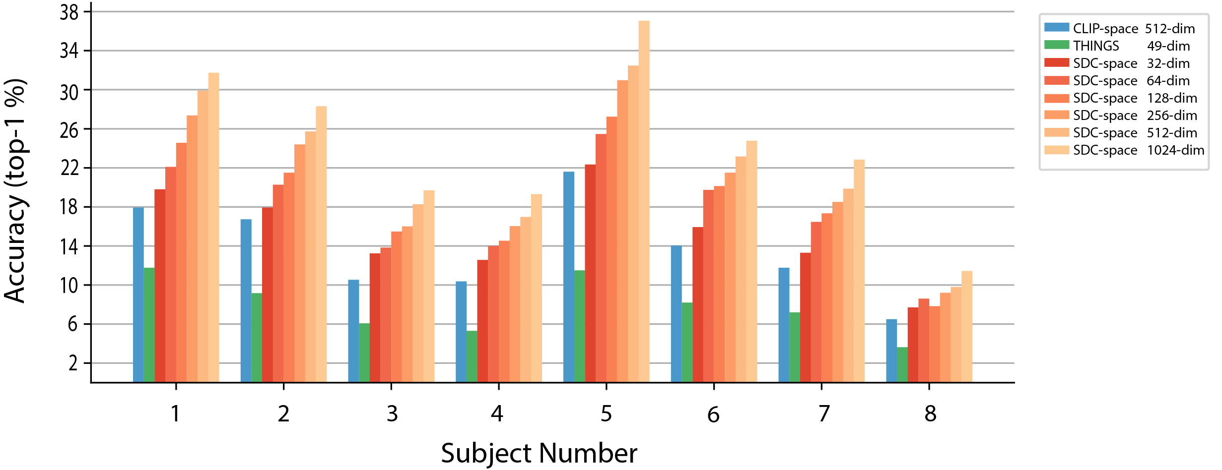
Because CLIP was trained on images and text, it is an efficient embedding space for those modalities. However, we are interested in the dimensions of meaning available in images that are decodable from fMRI recordings. To explore the brain-decodable dimensions of meaning in CLIP space we pursued two directions. First, we learned a mapping to transform CLIP into a pre-existing 49-dimensional model which was trained to on human behavioral responses to naturalistic image data from the THINGS-initiative (Hebart et al., 2023). Second, to find dimensions of meaning specifically available in fMRI data, we explored several possible linear projections of the brain-decoded CLIP embeddings, . This method, which combines predicted CLIP embeddings across participants, produced dramatic increases in top-1 accuracy over the original CLIP space and the THINGS space transformation of CLIP (Figure 1(b))
3.1 THINGS Concepts
THINGS Experiment
The THINGS-Images database consists of 1854 object classes with 12 images per class (Hebart et al., 2023). These images were used to gather approximately 1.46 million responses to an odd-one-out task, during which MTurk workers were asked to select the one image (from a group of 3) that least belonged in the group. These responses were then used to learn THINGS object embeddings , . Initially, is randomly initialized. Then, for each triplet of classes , and the human-chosen odd one out (), the model is trained to maximize the dot products of the embeddings for the non-odd-one-out concepts (), and minimize the other two dot products ( and ). The model is constrained ensure non-negativity and encourage sparsity in . After training, contains 49 human-interpretable dimensions that are most important for performing the odd-one-out similarity judgments. These 49 dimensions were assigned semantic labels by hand.
Translation from CLIP to THINGS space
We trained a function to map from CLIP space to THINGS space. To train this mapping, all 12 images for each of the 1,854 Things object classes are passed into the CLIP image encoder to obtain . We then averaged CLIP embeddings for all images within an object class to obtain . These averaged embeddings are used to fit a linear ridge regression model:
| (2) |
Because the THINGS-embeddings are constrained to be non-negative, after training we introduced an additional ReLU operation, , and further finetuned . Empirical results for this fine tuning can be seen in the Supplementary Material. The CLIP-to-THINGS mapping function allows us to map CLIP embeddings derived from NSD stimulus images to THINGS space. In addition, we can use brain responses to those images passed through the decoder to derive decoded THINGS embeddings directly from the NSD fMRI.
Results for computing top-k accuracy in THINGS space appear in Figure 2 (green bar). Decoding performance in THINGS space is lower than in the original CLIP space. This implies that the THINGS concepts, originally derived from behavioral data, do not sufficiently capture the visual concepts available in CLIP space that are decodable from fMRI. This motivates the search for a new embedding space tuned specifically for the decodable concepts shared amongst all participants in the NSD dataset.
3.2 Finding Shared Decodable Concepts (SDC)
In this section, we describe our method for deriving a transformation of CLIP space that reveals brain-decodable interpretable dimensions that are shared across participants. First, each participant’s brain decoded and ground truth stimulus representations are concatenated into shared matrices . The function that maps CLIP space to a shared decodable concept space (SDC) where is the chosen dimensionality of the SDC-space. Similar to , the mapping function is defined as a multiplication by a weight matrix followed by a ReLU, i.e. . The weight matrix is found by optimizing
| (3) |
The weight matrix is randomly initialized and trained for 10,000 iterations using the Adam optimizer, a batch size of 3,000, learning rate 2e-4. A leaky ReLU with a negative slope of 0.05 is used during optimization because it encourages convergence of the SDC space components. The SDC model is fit for different numbers of components .
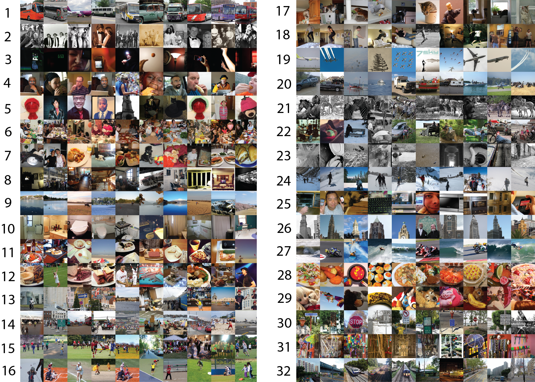
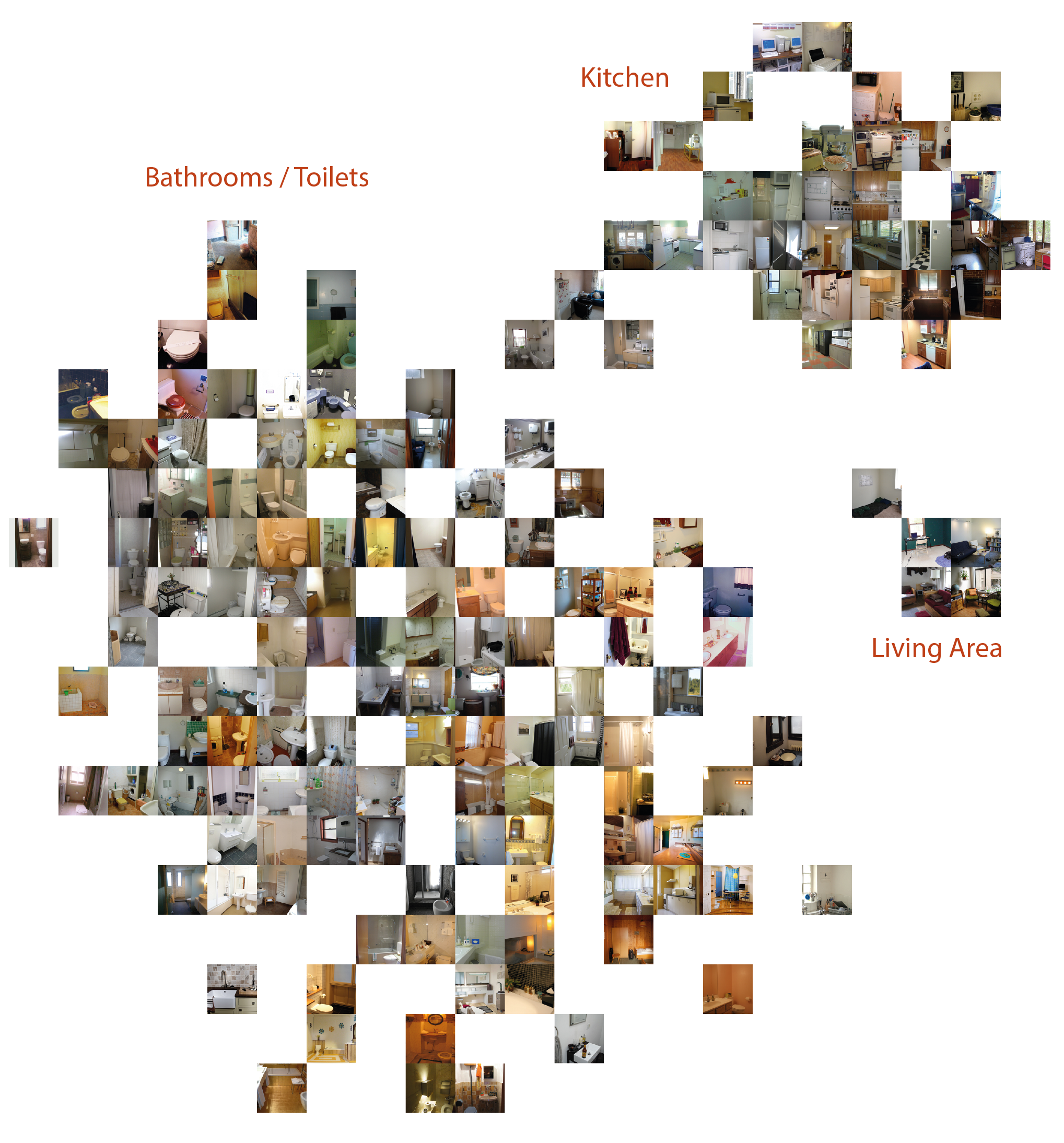
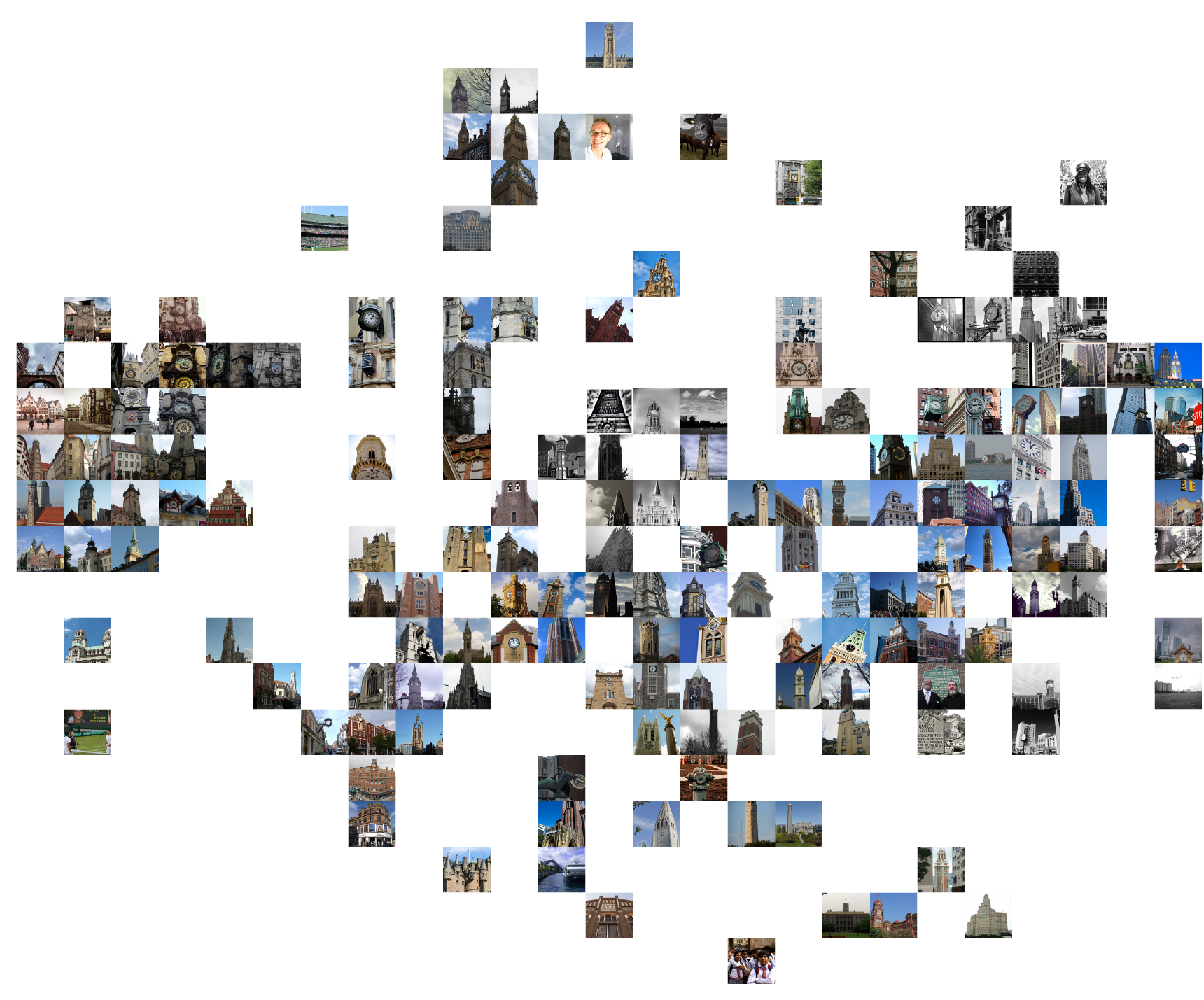
Results for computing top-k accuracy in SDC space appear in Figure 2 (orange bars). Decoding performance in SDC space is higher than in the original CLIP space, and grows with increasing dimension. This implies that there are visual concepts available in CLIP space that are decodable from fMRI, but that CLIP contains information not available from the fMRI in our experimental setting. Figure 3 depicts the top 10 nearest-neighbour images for each learned concept vector, namely, each row in with . We then visualized a selection of concept vectors by projecting a larger selection of nearest-neighbours () down to 2-dimensional space using t-distributed stochastic neighbour embedding (t-SNE) projection. Figure 4 outlines two dimensions we found to represent animal concepts. Further dimensions associated with other semantically-coherent concepts are given in the Appendix: food (Fig. 12), household rooms (Fig. 14), buildings (Fig. 15) and images associated with strong uniform backgrounds (skies, snow-covered mountains etc.) (Fig. 13). The next sections explore this new SDC space for consistency and specificity across participants.
4 Brain-Decodable Concepts that Consistently Correspond to Specific Brain areas
We localize each concept dimension from our learned matrix to a small subset of voxels with a masking procedure that selects sparse voxel sub-groups. We investigate the spatial contiguity and sparsity of concept voxel sub-groups, and the cross-participant and cross-concept consistency via participant- and concept-specific voxel masks, . To test consistency across participants, we define a new metric which takes into account the fractional overlap of voxels present in concept masks across the ROIs calculated using the Human Connectome Project Atlas (HCP-MMP1) for each participant. This allows us to determine broad spatial similarity patterns across participants in their native brain spaces (not aligned to an average brain template), allowing smaller voxel subgroups tuned to finer-grained semantic distinctions to be compared, while maintaining idiosyncratic participant-specific functional anatomy.
4.1 Finding Concept Brain Areas
For each CLIP concept vector from and , our objective is to find a sparse binary voxel mask ( is the number of voxels) that defines a set of voxels that support the decodability of the concept for participant . The masks are derived by fitting a LASSO regression model
| (4) |
Here is the number of data points and the regularization hyperparameter is used for all concept masks. All non-zero values in are set to to derive the binary mask that is used for further analysis in this section.
4.2 Evaluation of SDC concept masks
Mask Concept Specificity
An initial question is whether the brain regions represented by are truly specific to their corresponding concept vectors , or do they equally support the decodability of other concepts where ? To help answer this, we measure the relative change in brain decodability for a concept after applying a mask . The matrix of relative changes in brain decodability for a participant is constructed as follows:
| (5) |
where denotes element-wise multiplication and is the Pearson correlation coefficient. Then the participant-specific are averaged across participants to obtain which is displayed in Figure 7.
Cross Participant Consistency
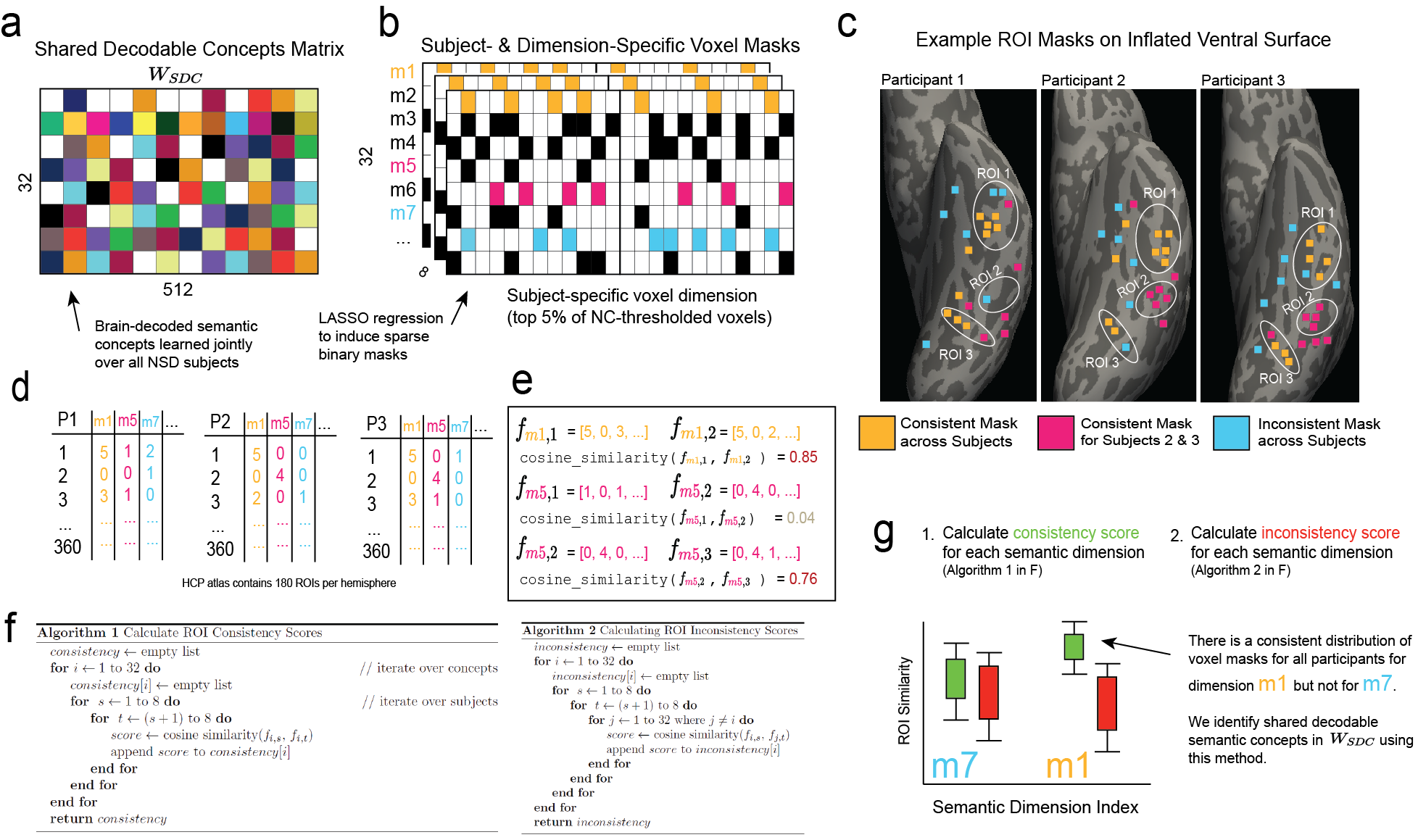
Next, we investigate whether the masks exhibit consistency in their spatial locations within the brain across participants. The highly sparse and disjoint nature of the masks motivated the use of an ROI-based similarity measure. The HCP_MMP1 atlas parcellates the cortical surface into 180 distinct regions per hemisphere. We used this atlas to define ROI fraction vectors for each concept mask . Each element in represents the number of voxels in that intersect a particular ROI in the atlas, divided by the total number of voxels in . The similarity of mask regions can be compared across participants by taking the cosine similarity between ROI fraction vectors, i.e. where index concepts and index participants. Figure 5 outlines the method we use to identify shared decodable concepts.
Using our shared decodable concepts matrix , (Fig. 5a), we use LASSO regularization to induce a participant-specific subset of voxels we call a voxel mask, such that each individual participant has a sparse voxel mask for each dimension of (Fig. 5b). The dimensionalities of the masks per-participant and per-mask are given in A.2. We demonstrate the procedure by selecting 3 synthetic example dimensions for purposes of illustration, , and for three participants in the fMRI dataset. In Fig-5c we show an example of how these voxel masks for 3 participants might be spatially organised along the inflated ventral surface (images generated using Freesurfer’s Freeview program (Fischl, 2012)). Dimension (orange voxels) is highly consistent across participants, meaning that it frequently appears in ROI-1 and ROI-3 of each participant. Dimension (magenta voxels) is consistent between participants 2 and 3, both appearing in ROI-2 but not in ROI-2 in Participant 1. This represents partial consistency. Finally, dimension (blue voxels) represents a situation where the spatial organization of the mask does not intersect any defined ROI consistently across participants. By taking the 360 automatically-generated ROIs (180 from each hemisphere) from the Human Connectome Project (HCP) Atlas (Glasser et al., 2016), calculated by Freesurfer’s recon-all program, we count the number of voxels in each mask that intersect with each ROI and for each participant’s set of masks. This yields a 360-dimensional vector for each participant and each mask (Figure 5d). We then calculate the cosine similarity between these vectors in order to determine if there is a consistent shared representation of mask voxels across the ROIs as shown in Fig. 5e. For each dimension of , we calculate a list of consistent (high cosine similarity) and inconsistent (low cosine similarity) scores according to the algorithms given in Fig. 5f.
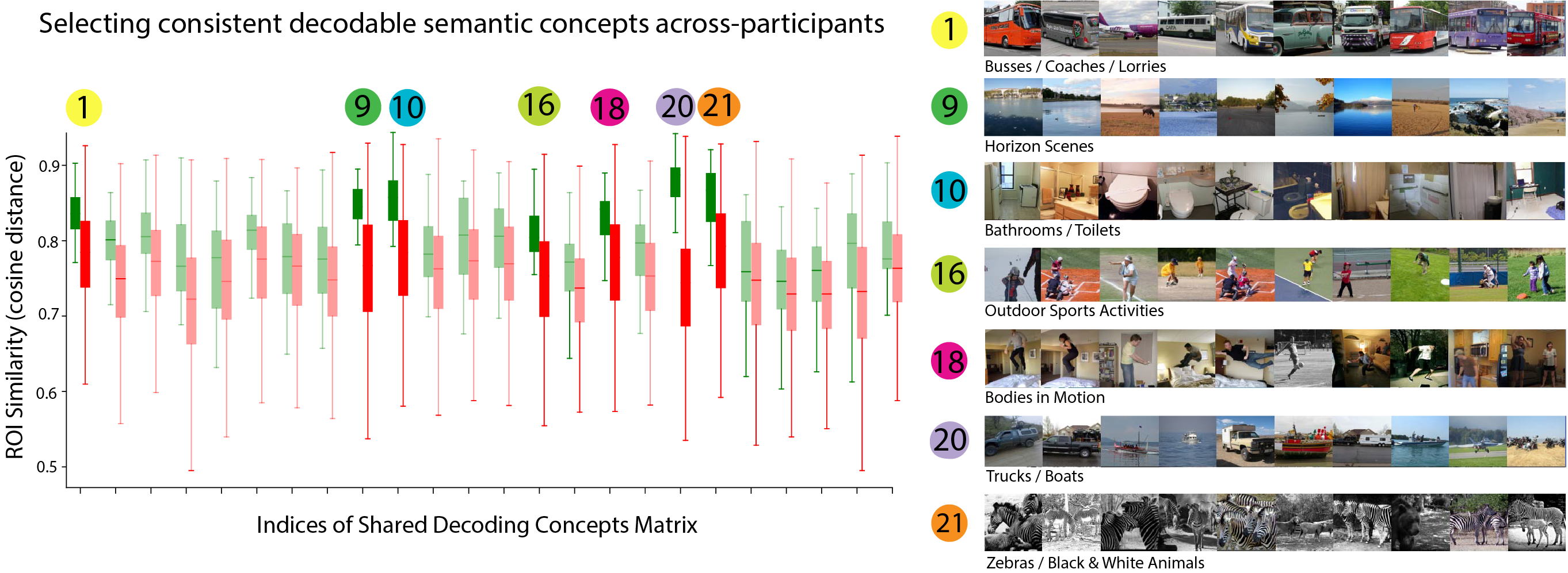
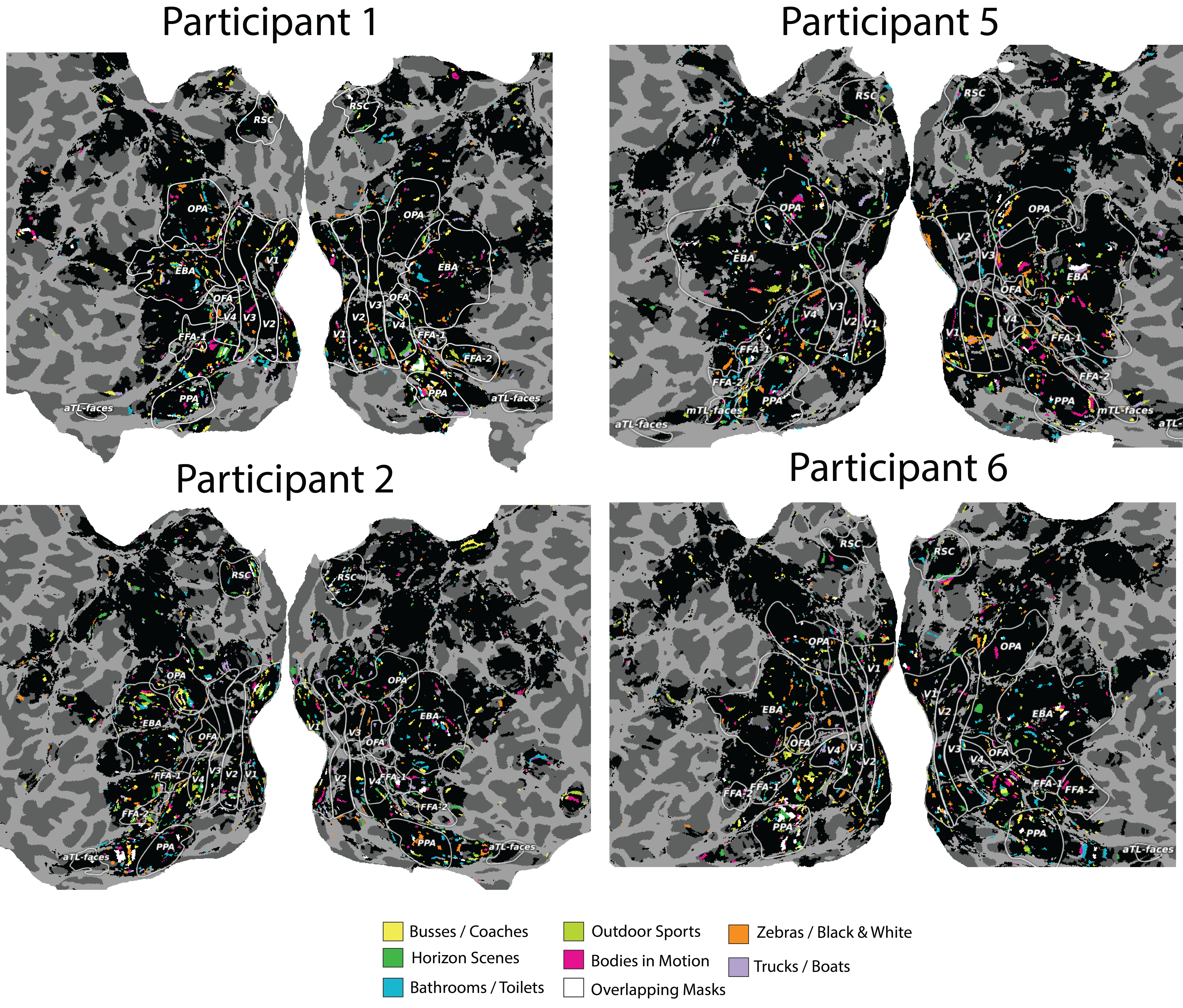
By comparing the distributions of both sets of results, we identify dimensions that share stable mask distributions across participants (Fig. 5g). For some dimensions of our optimized matrix, we find greatly increased consistency across participants. We selected the top 7 dimensions and plot the 10 most associated images for that dimension in Figure 6. These shared decodable concept dimensions have associated images that are superficially very distinct but have a clearly consistent semantic interpretation.
Voxel subselection
The mask optimization procedure does not explicitly encourage the discovery of contiguous voxel subgroups, yet this is exactly what we find when generating masks for each of the decodable semantic concepts. This allows us to explore mask distributions across ROIs associated with specific semantically congruent stimuli, such as dimensions often used in fMRI localizer scans. We consistently find that semantic dimensions in our shared decoding space that contain prominent faces, bodies and places have contiguous mask locations in the expected ROIs. These voxel subgroups in our results occupy much smaller and fine-grained areas of ROIs found in localizer experiments, which may be related to processing the various fine-grained semantic distinctions. We expand on this analysis in Appendix A.1. Using the dimensions we found to be most consistent across participants (Figure 6: right), we further explore the voxel mask locations to identify which brain areas support the semantic dimensions of that are consistent across participants.
4.3 Identifying Brain Regions Underpinning Fine-Grained Shared Decodable Concepts
We visualized the spatial locations of voxel masks for key semantic dimensions which we found to be consistent across subjects in Figures 6 and 7. We noted several consistencies and plot color-coded voxel masks for a sample of 4 NSD participants in Figure 8. For Participant 1, we found an area where the masks for dimensions 16 and 18 largely overlap. The top images in dimension 16 depict people performing a variety of sports activities, and dimension 18 mainly depicts people bodily motion (i.e. jumping). The brain area where the two corresponding maps overlap is PFcm, which has been associated with the action observation network (Caspers et al., 2010, Urgen and Orban, 2021). We highlight this region later in Figure 10. In the same participant, we also note that masks for dimensions 9 and 20 overlap substantially. The top images in those dimensions contain horizon scenes and trucks/boats, respectively, and are conceptually linked by their outdoor settings. The brain area where these maps overlap is area TF of parahippocampal cortex: importantly, the parahippocampal place area (PPA) is known to represent places and identification of such voxel masks points to specialized subsections that could underlie more fine-grained representations relating to the broad semantic concept of place.
The t-SNE results in Section 3.2 (and Appendix A.3) show remarkably coherent semantic networks containing hierarchical representations that cluster together in human-interpretable ways. We further explore the spatial organization of some of these dimensions by inspecting the participant-specific voxel masks learned for these dimensions in order to derive hypotheses for future work out of our data-driven approach.
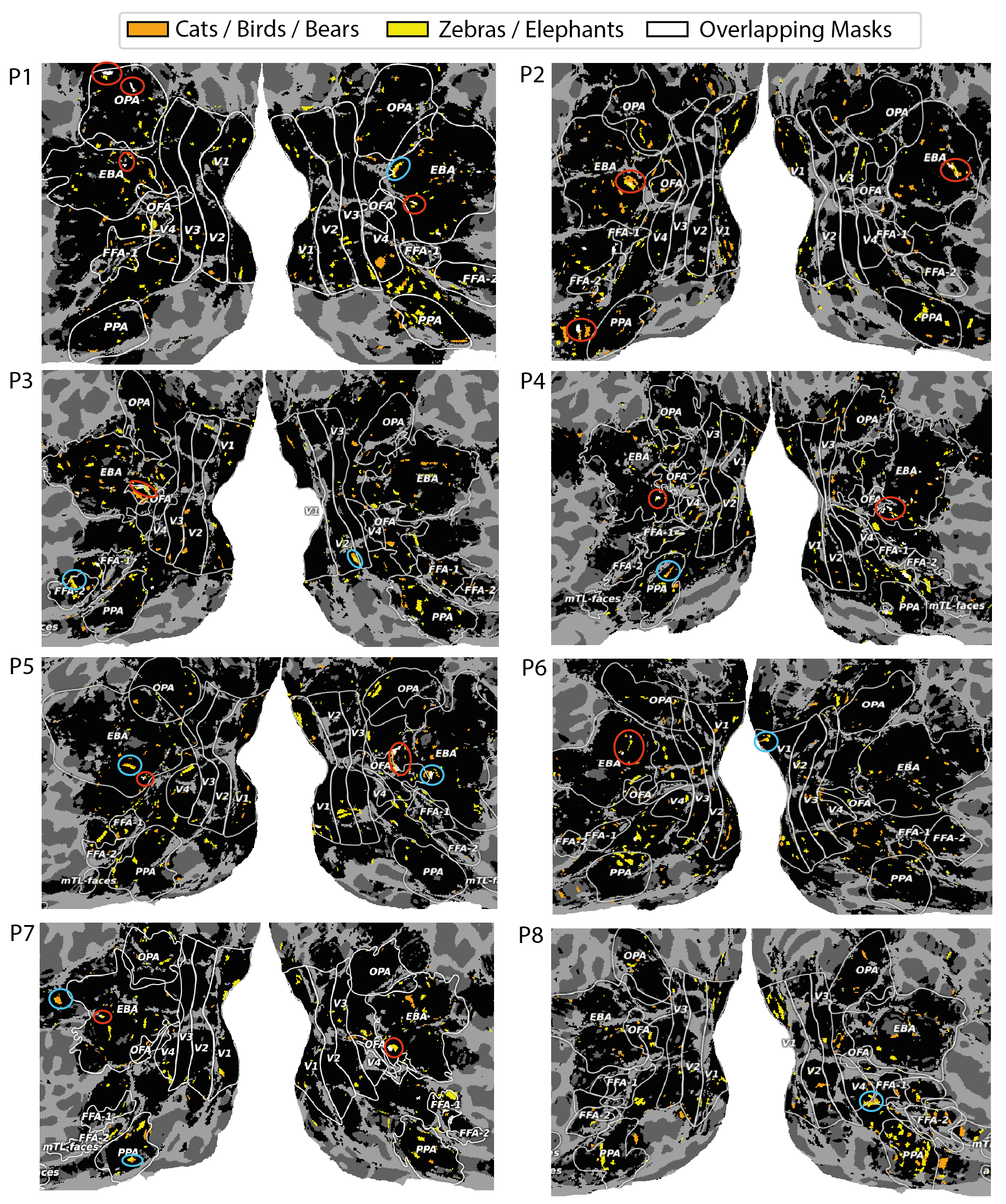
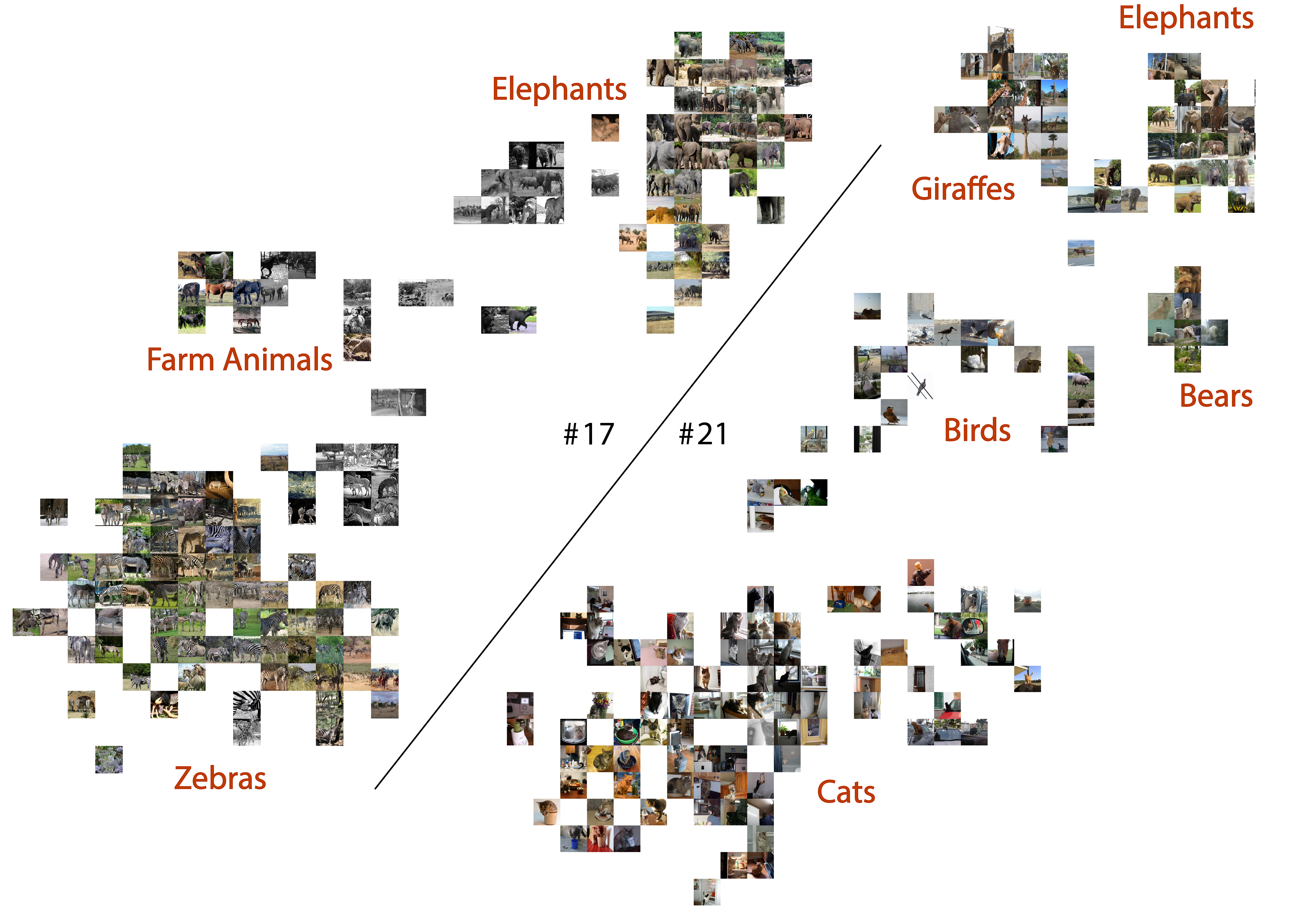
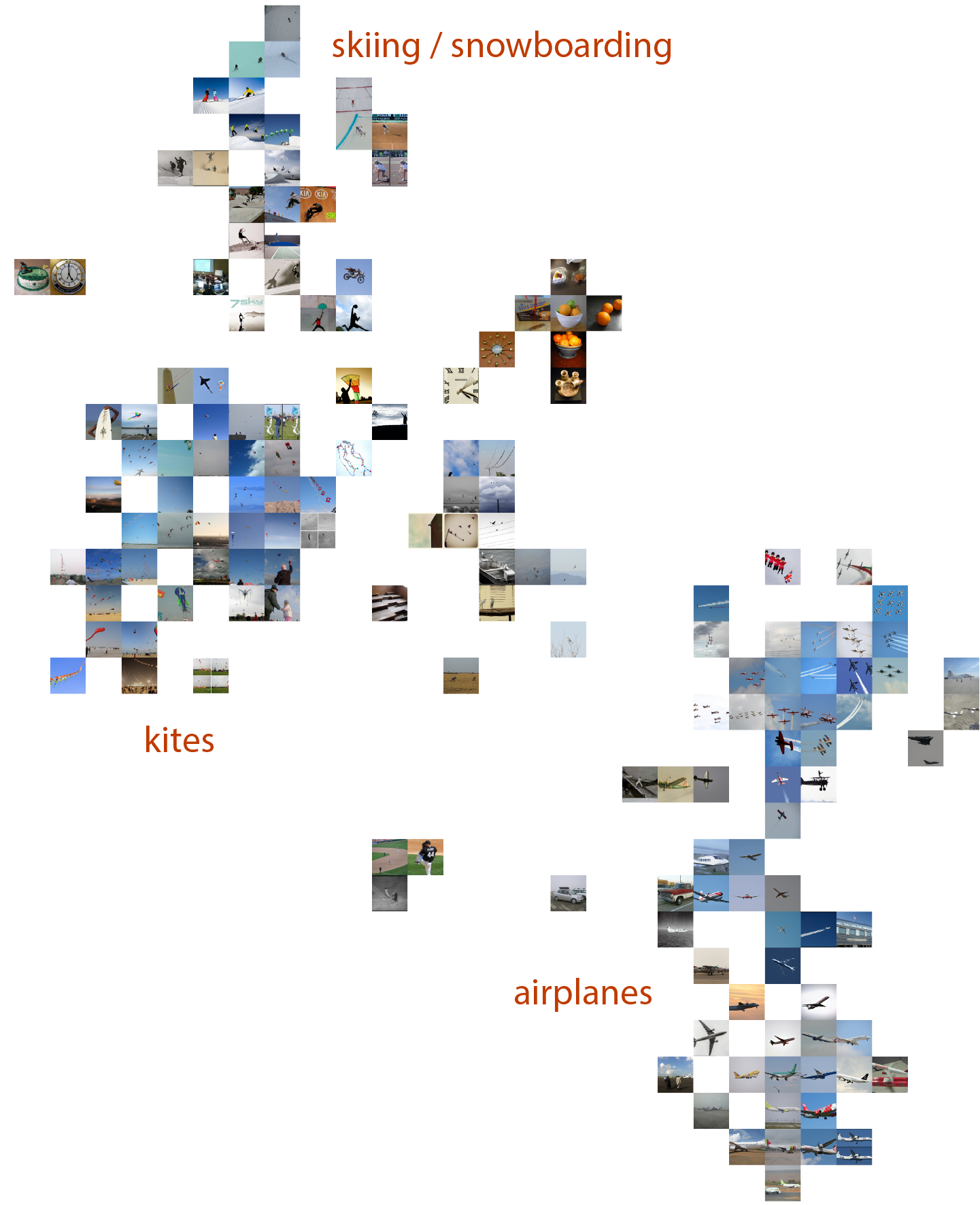
Figure 4 showed two dimensions related to animals, in which one (dimension 17) contained clusters of cats, birds, bears, giraffes and elephants, while the other (dimension 21) contained clusters of zebras, farm animals and (again) elephants. Figure 9 shows the 8 participants’ voxel masks for these two dimensions. We first note that the masks are largely non-overlapping, but we do see bilateral sections of the EBA selected (red circles) consistently across participants, though often at different extrema of the EBA’s boundaries, reflecting an individual’s functional / anatomical individuality. Furthermore, for participants 1,2,3,5,6,8 we see much greater voxel selection in PPA for dimension 21 (yellow), which is the dimension that represents animals in the wild, compared to dimension 17, which is largely related to indoor cats or birds in the sky. We also find in some participants that voxel masks are learned that share adjoining yet non-overlapping continua (blue circles). We believe this an interesting finding, after discovering the most selective images associated with these components were semantically linked to animals. We perform the same analysis on the food dimension that we identified (dimension 28) in Appendix A.4.
4.3.1 Identifying Within-Participant Brain Regions Underpinning Shared Semantics
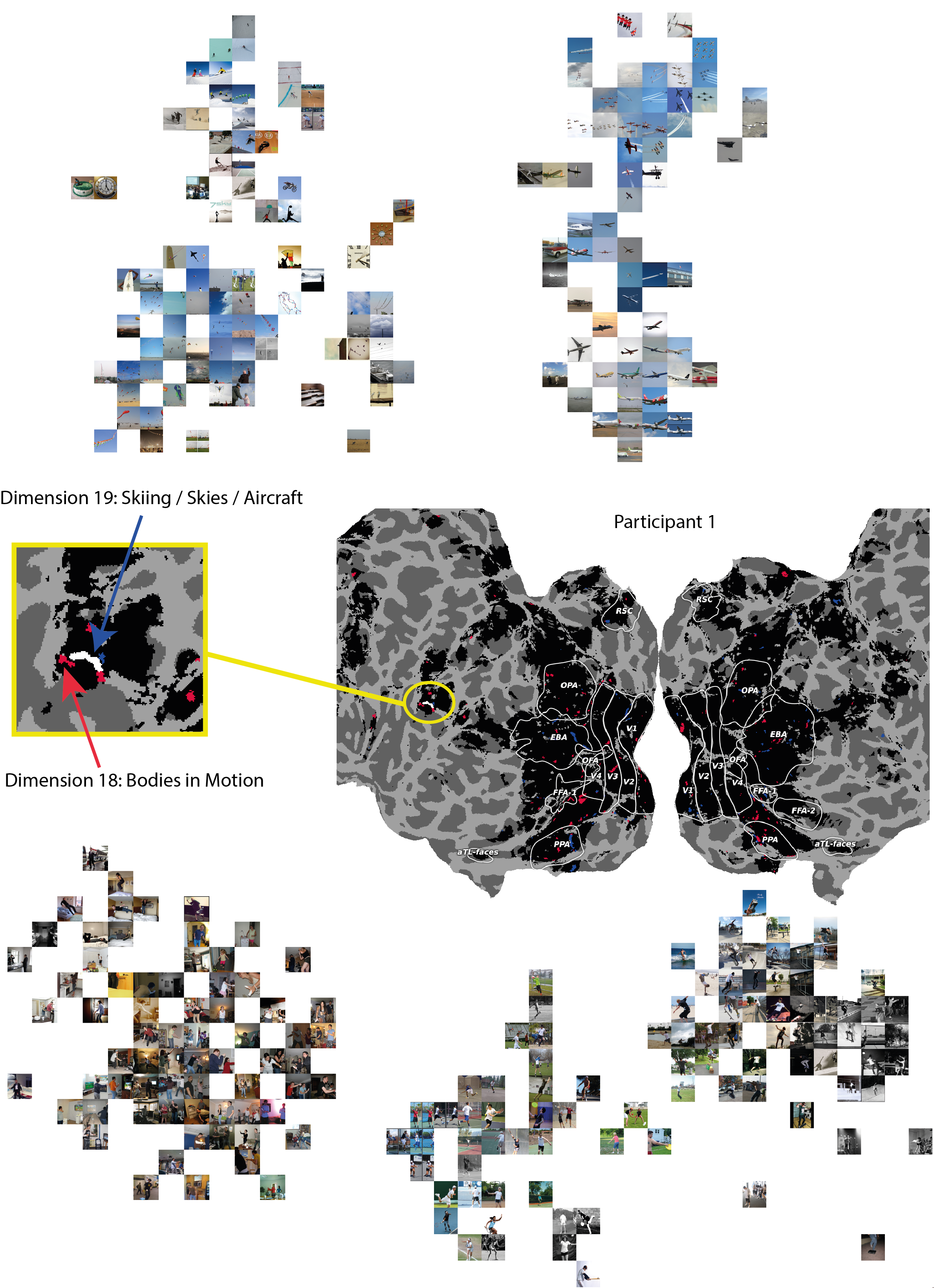
In Section 4.3 it was suggested that Participant 1’s voxel mask distribution to dimension 10 ("bodies in motion") had found a large continuous patch of voxels in region PFcm, a region that had previously been linked to bilateral activation when processing action / activity (Urgen and Orban, 2021). This voxel mask largely overlapped with the voxel mask for dimension 16 ("outdoor sports"). We looked for other semantic concepts that implied movement / action and selected dimension 19, due to the presence of skiers, snowboarders and skateboarders in the t-SNE visualisation of the top images in that cluster (see A.3.2). Encouragingly, we find that this semantic dimension has also induced a learned voxel mask that overlaps with the same patch of cortex in this area of interest. This appears to serve as a signature of observed action when processing images, given the varied surface level features of the visual images in each dimension. Figure 10 shows the flat map representation of Participant 1’s cortex (middle), with the voxel mask locations for these two dimensions overlaid. We further examined the t-SNE clusters for these dimensions (top: dimension 19, bottom: dimension 18). When only plotting the top-10 nearest neighbours earlier in Figure 3, we only identified the concepts implying body motion indoors, but extending this to a larger numbers of images, we also see that this dimension captures bodies in motion during sports, beyond just jumping. We note that virtually all images connected to dimension 18 involve a form of action, while a portion of dimension 19 also overlap in the same semantic regions (skiing, snowboarding, skateboarding, kite-flying). We find overlap in the left PFcm region, which has been previously associated with action observation (yellow box). The patch of cortex where both dimension masks overlap reveal that the mask for dimension 19 is smaller than that of dimension 18, which makes sense as only a subset of the images associated with dimension 19 are specific to action observation.
These t-SNE clusters reveal two sets of images that are superficially different but we find semantic overlaps that can be linked to adjoining / overlapping patches of cortex that sparse voxel masks can detect, which can then be related to prior literature that previously found evidence that the same region supports the same semantic overlap we observed in the image dimensions, namely action observation. We find that for a few participants that the contrast of these two dimensions results in overlapping continuous strips in PPA (not shown). We envisage that the method we present to identify shared decodable concepts can also be used to map out within-participant fine-grained semantic networks and we demonstrate an example of this on our initial results here.
5 Discussion
We introduced a new data-driven method that uses the CLIP language-image foundation model (Radford et al., 2021) to identify sets of voxels in the human brain that are specialized for representing different concepts in images. Using this method, we identified several putative new concept-encoding networks that were consistent between individuals. Our method also identified concept-encoding regions that were previously known (e.g., regions specialized for faces, places, and food), which increased our confidence in the new regions uncovered by our method.
Importantly, our new method enables us to compare fine-grained participant-specific concept-encoding networks (defined as sets of voxels) without needing to apply any compression to the brain imaging data. These networks can then be mapped to 180 different anatomically-defined brain regions in each hemisphere, enabling us to relate our concept-encoding networks to known brain anatomy. At the same time, by virtue of its fine-grained resolution, our method can identify concept-encoding networks that span multiple anatomical brain regions, and those that occupy portions of known brain regions.
Among the new concepts-encoding networks we identified are networks specialized for jumping bodies, transport, scenes with strong horizons, room internal (toilet/bathroom). These are clearly important concepts, but their representations are ones that would not be readily identified using standard methods that attempt to tie brain areas to semantic concepts. This is because the space of potential concepts to explore is so large that a hypothesis-driven “guess and check” approach is likely to miss many important concepts. For this reason, our data-driven approach represents an important advance, and highlights the utility of modern AI systems (e.g., the CLIP language-image foundation model) for advancing cognitive neuroscience. Importantly, the method we introduced is quite general: while we have applied it here to CLIP embeddings and fMRI data, future work could apply the same method to embeddings generated by other AI systems (not just CLIP), and/or to other brain recording modalities (not just fMRI).
All neural recordings are from a previously released public dataset (Allen et al., 2022). The recordings were collected with the oversight of the institutional review boards at the institute where the experiments were performed. Our work has the potential to enable new methods for decoding human brain activity using non-invasive methods. Such methods could have substantial impacts on society. On the positive side, these methods could assist in diagnosing psychiatric disorders, or in helping individuals with locked-in syndrome or related disorders to better communicate. On the other hand, the same brain decoding methods could pose privacy concerns. As with all emerging technologies, responsible deployment is needed in order for society as a whole to obtain maximum benefit while mitigating risk.
There are several limitations of this work, and decoding experiments in general. Firstly, we use fMRI, and so can only recover the shared decodable concepts available in that fMRI space. That is, if concepts are not encoded by the BOLD signal as measurable by fMRI, we will not be able to recover them. On the other hand, the methods we develop here could be applied to other neural recording modalities that more directly measure neural activity, including electrocorticography. Consequently, this first limitation is one that could be overcome in future studies.
Secondly, we are also only able to uncover concepts that appear in the CLIP space spanned by the images in the stimulus set. This means that, while our method is more flexible than the hypothesis-driven ones used by previous studies (Kanwisher et al., 1997), some important concept representations could still be missed by our method. Future work could address this limitation by using even larger stimulus sets. Finally, we report on a few probable localizations of concepts. These provide clear hypotheses for future experiments that should be targeted at attempting to confirm these findings. This emphasizes that our new data-driven method is not a replacement for the hypothesis-driven approach to identifying concept-encoding regions in the human brain: rather, it serves as a data-driven hypothesis generator that can accelerate the task of understanding how our brains represent important information about the world around us.
References
- Allen et al. (2022) E. J. Allen, G. St-Yves, Y. Wu, J. L. Breedlove, J. S. Prince, L. T. Dowdle, M. Nau, B. Caron, F. Pestilli, I. Charest, J. B. Hutchinson, T. Naselaris, and K. Kay. A massive 7t fmri dataset to bridge cognitive neuroscience and artificial intelligence. Nature Neuroscience, 25(1), 2022. doi: 10.1038/s41593-021-00962-x.
- Caspers et al. (2010) S. Caspers, K. Zilles, A. R. Laird, and S. B. Eickhoff. Ale meta-analysis of action observation and imitation in the human brain. NeuroImage, 50(3):1148–1167, 2010. ISSN 1053-8119. doi: https://doi.org/10.1016/j.neuroimage.2009.12.112. URL https://www.sciencedirect.com/science/article/pii/S1053811909014013.
- Epstein and Kanwisher (1998) R. Epstein and N. Kanwisher. A cortical representation of the local visual environment. Nature, 392(6676):598–601, 1998.
- Fischl (2012) B. Fischl. Freesurfer. NeuroImage, 62(2):774–781, 2012. ISSN 1053-8119. 20 YEARS OF fMRI.
- Gao et al. (2015) J. S. Gao, A. G. Huth, M. D. Lescroart, and J. L. Gallant. Pycortex: an interactive surface visualizer for fmri. Frontiers in Neuroinformatics, 9, 2015. ISSN 1662-5196. doi: 10.3389/fninf.2015.00023.
- Glasser et al. (2016) M. Glasser, T. Coalson, E. Robinson, C. Hacker, J. Harwell, E. Yacoub, K. Ugurbil, J. Andersson, C. Beckmann, M. Jenkinson, S. Smith, and D. v. Essen. A multi-modal parcellation of human cerebral cortex. Nature (London), 536(7615):171–8, 2016. ISSN 0028-0836.
- Hamilton and Huth (2020) L. S. Hamilton and A. G. Huth. The revolution will not be controlled: natural stimuli in speech neuroscience. Language, Cognition and Neuroscience, 35(5):573–582, 2020. doi: 10.1080/23273798.2018.1499946. PMID: 32656294.
- Hanson and Halchenko (2008) S. J. Hanson and Y. O. Halchenko. Brain reading using full brain support vector machines for object recognition: there is no “face” identification area. Neural Computation, 20:486–503, 2008. ISSN 0899-7667. doi: 10.1162/neco.2007.09-06-340.
- Haxby et al. (2001) J. V. Haxby, M. I. Gobbini, M. L. Furey, A. Ishai, J. L. Schouten, and P. Pietrini. Distributed and overlapping representations of faces and objects in ventral temporal cortex. Science, 293(5539):2425–2430, 2001.
- Hebart et al. (2023) M. Hebart, O. Contier, L. Teichmann, A. H. Rockter, C. Y. Zheng, A. Kidder, A. Corriveau, M. Vaziri-Pashkam, and C. I. Baker. Things-data, a multimodal collection of large-scale datasets for investigating object representations in human brain and behavior. eLife, 12, 2023.
- Hubel and Wiesel (1959) D. H. Hubel and T. N. Wiesel. Receptive fields of single neurons in the cat’s striate cortex. Journal of Physiology, 148:574–591, 1959.
- Jain et al. (2023) N. Jain, A. Wang, M. M. Henderson, R. Lin, J. S. Prince, M. J. Tarr, and L. Wehbe. Selectivity for food in human ventral visual cortex. Communications Biology, 6(1), 2023. doi: 10.1038/s42003-023-04546-2.
- Kanwisher et al. (1997) N. Kanwisher, J. McDermott, and M. M. Chun. The fusiform face area: A module in human extrastriate cortex specialized for face perception. Journal of Neuroscience, 17(11):4302–4311, 1997. ISSN 0270-6474. doi: 10.1523/JNEUROSCI.17-11-04302.1997. URL https://www.jneurosci.org/content/17/11/4302.
- Khosla et al. (2022) M. Khosla, N. A. R. Murty, and N. Kanwisher. A highly selective response to food in human visual cortex revealed by hypothesis-free voxel decomposition. Current Biology, 32(19):4159–4171, 2022.
- Kriegeskorte et al. (2009) N. Kriegeskorte, W. Simmons, P. Bellgowan, and C. Baker. Circular analysis in systems neuroscience: The dangers of double dipping. Nature neuroscience, 12:535–40, 05 2009.
- Lin et al. (2014) T.-Y. Lin, M. Maire, S. Belongie, L. Bourdev, R. Girshick, J. Hays, P. Perona, D. Ramanan, C. L. Zitnick, and P. Dollár. Microsoft coco: Common objects in context, 2014. cite arxiv:1405.0312Comment: 1) updated annotation pipeline description and figures; 2) added new section describing datasets splits; 3) updated author list.
- Matusz et al. (2019) P. J. Matusz, S. Dikker, A. G. Huth, and C. Perrodin. Are We Ready for Real-world Neuroscience? Journal of Cognitive Neuroscience, 31(3):327–338, 03 2019. ISSN 0898-929X. doi: 10.1162/jocn_e_01276. URL https://doi.org/10.1162/jocn\_e\_01276.
- McCandliss et al. (2003) B. D. McCandliss, L. Cohen, and S. Dehaene. The visual word form area: expertise for reading in the fusiform gyrus. Trends in Cognitive Sciences, 7(7):293–299, 2003. ISSN 1364-6613. doi: https://doi.org/10.1016/S1364-6613(03)00134-7. URL https://www.sciencedirect.com/science/article/pii/S1364661303001347.
- Noppeney (2008) U. Noppeney. The neural systems of tool and action semantics: A perspective from functional imaging. Journal of Physiology-Paris, 102(1):40–49, 2008.
- Pennock et al. (2023) I. M. Pennock, C. Racey, E. J. Allen, Y. Wu, T. Naselaris, K. N. Kay, A. Franklin, and J. M. Bosten. Color-biased regions in the ventral visual pathway are food selective. Current Biology, 33(1):134–146, 2023.
- Prince et al. (2022) J. S. Prince, I. Charest, J. W. Kurzawski, J. A. Pyles, M. J. Tarr, and K. N. Kay. Improving the accuracy of single-trial fmri response estimates using glmsingle. eLife, 11:e77599, nov 2022. ISSN 2050-084X. doi: 10.7554/eLife.77599.
- Radford et al. (2021) A. Radford, J. W. Kim, C. Hallacy, A. Ramesh, G. Goh, S. Agarwal, G. Sastry, A. Askell, P. Mishkin, J. Clark, G. Krueger, and I. Sutskever. Learning transferable visual models from natural language supervision. CoRR, abs/2103.00020, 2021.
- Urgen and Orban (2021) B. A. Urgen and G. A. Orban. The unique role of parietal cortex in action observation: Functional organization for communicative and manipulative actions. NeuroImage, 237:118220, 2021. ISSN 1053-8119. doi: https://doi.org/10.1016/j.neuroimage.2021.118220.
- van den Oord et al. (2018) A. van den Oord, Y. Li, and O. Vinyals. Representation learning with contrastive predictive coding. CoRR, abs/1807.03748, 2018.
Appendix A Appendix
A.1 Consistency Check with Faces, Bodies and Place Images
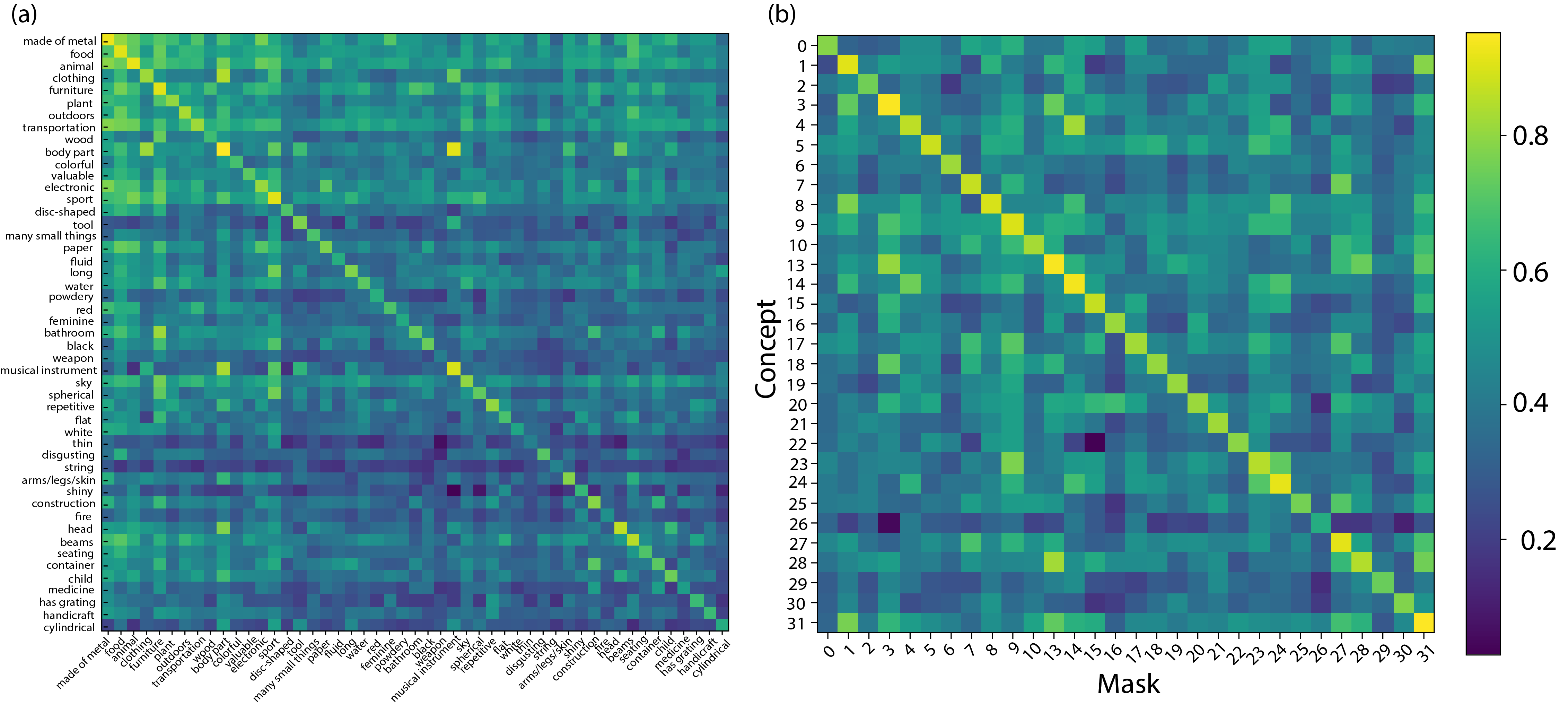
In order to verify that our masking procedure captures known functional localization of various high-level visual concepts, such as faces, places, and bodies, we use the functional localizer scans present in NSD for these categories and calculate the overlap with our participant- and dimension-specific voxel masks. To do this, we use our derived matrix of 32 concepts that are found via fMRI-decoding into CLIP-space, where each dimension represents a potentially shared decodable concept derived from brain responses, revealing the semantic tuning sensitivity to visual concepts that are found to be important. For each dimension of , we extract the top-10 CLIP images that are nearest neighbours to the fMRI-decoded CLIP embeddings. We then identify a set of indices that we expect to activate voxel locations in the participant-specific NSD functional localizer maps. We plot these flat maps for each participant (generated in PyCortex (Gao et al., 2015)) along with a histogram (average over participants) of voxel mask locations that overlap with areas associated with higher-level functional ventral visual cortex. Figure 3 shows the top-10 associated images with each of the shared decodable concepts. Figure 11 shows the participant-specific maps and averaged histogram.
From Figure 3, we associate the three high-level functional categories of interest to the following indices: , and .
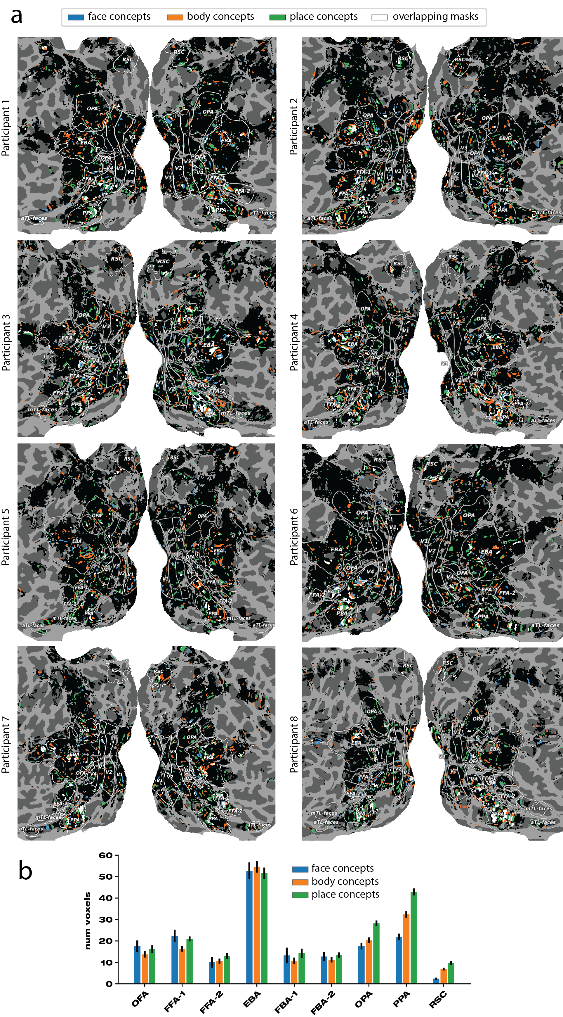
We clearly see that the mask dimensions for the higher-level concepts of faces, bodies and places do largely overlap with areas in which there is an a priori expectation of overlap. The images contained in NSD are largely confounded in that each image typically represents not just a single semantic concept. For example, images containing bodies will often contain faces, and most likely vice-versa (but head-shot images would be an exception to this). Furthermore, images of people are often in a place-context, whether inside, outside or in the proximity of an area. We see this fact in our mask distributions, too. In place images, such as dimension nine in Figure 3, where we see strong horizons, there is less confounding with face and body areas, as place contexts can easily exist without humans, but the reverse is often not true. We see the effect of this in that the place ROIs typically contain the closest association with pooled masks over our identified place dimensions (green bar is higher for OPA, PPA, RSC). These results show that even in a dataset of highly confounded images, the mask locations we derive in our procedure align well with results and expectations from prior literature, serving as a consistency check. Our procedure, however, reveals a vastly more fine-grained set of results across a wider range of cortex, linking (among other regions) functional ROIs together differentially, in order map out a distributed coding of semantically-complex visual inputs that can be used to explore semantic networks between-participants but also across-participants.
A.2 Specification of participant-Specific Data Dimensions
In Section 2.2 we specified that the number of voxels, per-participant, that passed the 5% noise ceiling thresholds were used as inputs into the initial fMRI decoding algorithm (converting fMRI data to brain-derived CLIP embeddings). The range of voxels that passed this threshold was specified to be in the range of 15-30k. Later on in Section 4.1, we discuss per-participant per-dimension masks (each participant has a specific mask for each of the shared decodable concepts derived in ). We specify the dimensionality of voxel inputs and mask dimensions for each participant in Table 1.
| P1 | P2 | P3 | P4 | P5 | P6 | P7 | P8 | |
| Voxels >NC | 26,753 | 27,790 | 20,562 | 21,417 | 25,490 | 30,542 | 15,648 | 15,265 |
| Mask 1 | 372 | 332 | 352 | 346 | 289 | 459 | 299 | 284 |
| Mask 2 | 224 | 243 | 251 | 235 | 194 | 216 | 190 | 176 |
| Mask 3 | 256 | 219 | 231 | 246 | 230 | 244 | 176 | 176 |
| Mask 4 | 253 | 232 | 254 | 229 | 217 | 268 | 215 | 180 |
| Mask 5 | 239 | 199 | 212 | 206 | 187 | 243 | 177 | 154 |
| Mask 6 | 322 | 290 | 324 | 284 | 274 | 354 | 278 | 299 |
| Mask 7 | 207 | 227 | 178 | 190 | 191 | 196 | 172 | 143 |
| Mask 8 | 258 | 254 | 250 | 188 | 219 | 244 | 208 | 175 |
| Mask 9 | 292 | 343 | 362 | 305 | 274 | 304 | 274 | 262 |
| Mask 10 | 342 | 353 | 345 | 323 | 363 | 404 | 327 | 288 |
| Mask 13 | 295 | 291 | 302 | 275 | 316 | 297 | 244 | 241 |
| Mask 14 | 272 | 254 | 286 | 261 | 242 | 236 | 223 | 232 |
| Mask 15 | 307 | 314 | 325 | 257 | 232 | 281 | 224 | 210 |
| Mask 16 | 255 | 235 | 242 | 233 | 203 | 226 | 222 | 155 |
| Mask 17 | 291 | 326 | 276 | 261 | 229 | 311 | 209 | 231 |
| Mask 18 | 245 | 304 | 346 | 280 | 263 | 308 | 282 | 222 |
| Mask 19 | 204 | 199 | 197 | 181 | 191 | 198 | 191 | 157 |
| Mask 20 | 225 | 240 | 179 | 197 | 225 | 223 | 165 | 185 |
| Mask 21 | 353 | 315 | 318 | 295 | 300 | 321 | 268 | 243 |
| Mask 22 | 249 | 241 | 245 | 277 | 235 | 262 | 204 | 180 |
| Mask 23 | 211 | 254 | 200 | 246 | 236 | 238 | 188 | 172 |
| Mask 24 | 282 | 275 | 256 | 228 | 220 | 238 | 229 | 196 |
| Mask 25 | 277 | 239 | 258 | 252 | 241 | 242 | 201 | 224 |
| Mask 26 | 266 | 287 | 237 | 232 | 234 | 267 | 216 | 173 |
| Mask 27 | 213 | 177 | 208 | 154 | 182 | 204 | 120 | 105 |
| Mask 28 | 316 | 295 | 294 | 282 | 262 | 314 | 236 | 254 |
| Mask 29 | 278 | 329 | 321 | 300 | 269 | 387 | 274 | 247 |
| Mask 30 | 232 | 209 | 212 | 226 | 211 | 229 | 226 | 211 |
| Mask 31 | 254 | 265 | 237 | 189 | 234 | 255 | 178 | 181 |
| Mask 32 | 253 | 302 | 303 | 278 | 269 | 327 | 258 | 246 |
We observe that the L1 regularization we apply in order to induce sparse masks results in similar voxel subset sizes for each shared decodable concept in irrespective of the number of voxels that passed the noise ceiling threshold and were used as inputs into the fMRI-decoding algorithm. Under our assumptions that a shared latent code across ROIs exists for shared decodable concepts, recovering broadly similar participant-specific and concept-specific mask voxel subset sizes is expected, although this does not itself mean they are similar in spatial distribution across the cortex. A beneficial feature of these masks is that they aren’t limited to exact spatial overlap within ROI regions. This allows for participant-specific anatomical and functional specialization to be identified by our analysis method. We assess this using an ROI-similarity metric that checks for cross-participant consistency.
A.3 Visualization of Shared Decodable Concept Clusters via t-SNE
In order to explore the semantic meanings of each of the 32 dimensions in the shared decodable concepts matrix presented in Section 3.2. of the main text, we transform the CLIP representations of the full set of 73,000 stimulus images into a shared decodable concept space, . The top 10 highest-scoring images on each dimension are selected and plotted in Figure 3. To allow for a more thorough investigation of individual dimensions, we select the top 250 highest-scoring images and embed their CLIP vectors in a 2-dimensional space using the t-distributed stochastic neighbor embedding (t-SNE) method. A selection of t-SNE visualizations are plotted in Figures 4, 15, 12, 13, 14. We plan to release the entire set of generated images and t-SNE projections upon manuscript acceptance. The t-SNE results in Section A.3 show remarkably coherent semantic networks containing hierarchical representations that cluster together in human-interpretable ways. We further explore the spatial organization of some of these dimensions by inspecting the participant-specific masks learned for these dimensions in order to derive hypotheses for future work out of our data-driven approach.
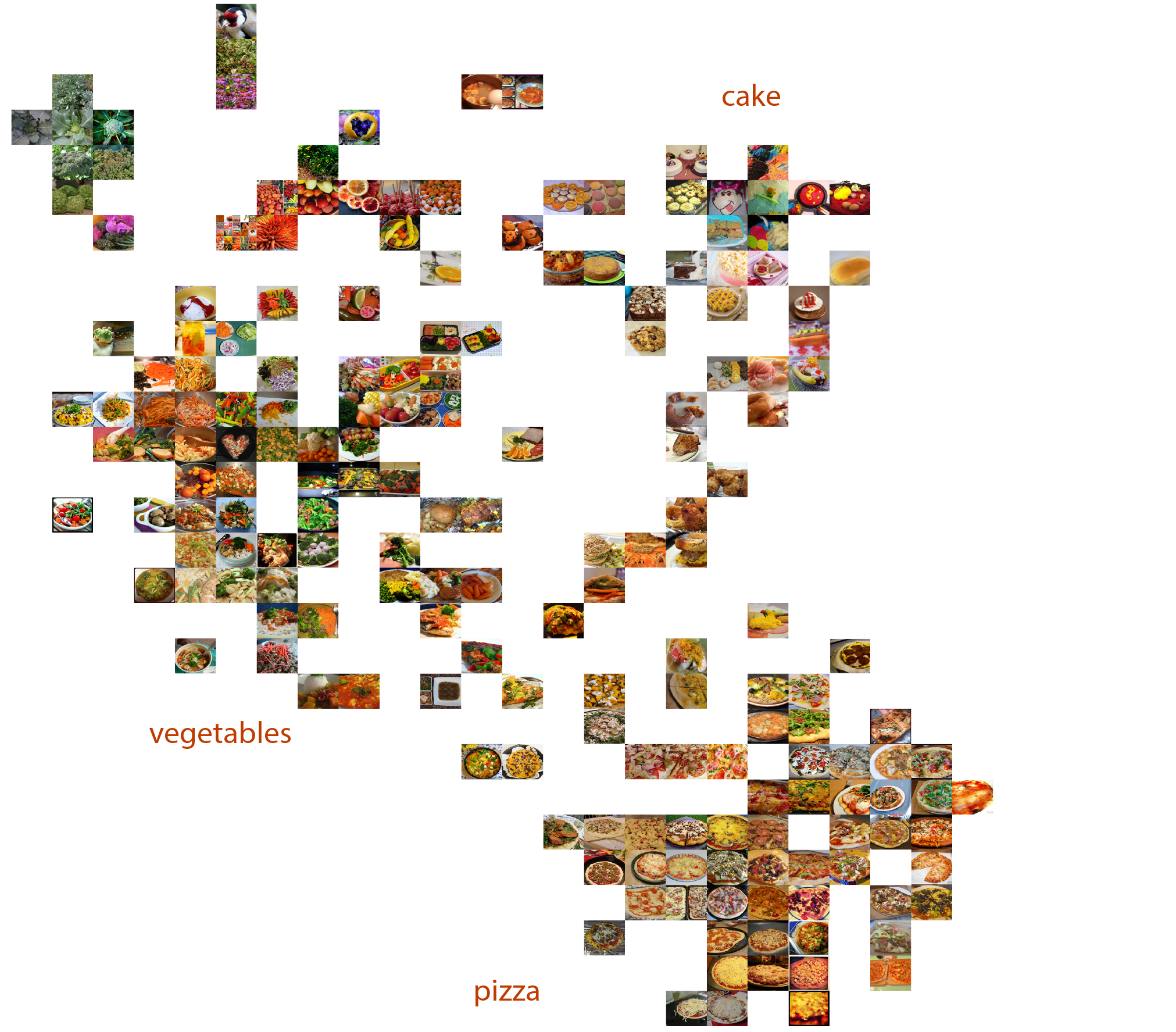
A.3.1 Food (Dimension 28)
Figure 12 shows a 2D t-SNE projection of the top 250 images from this dimension into clusters.
A.3.2 Skies (Dimension 19)
Figure 13 shows a 2D t-SNE projection of the top 250 images from this dimension into clusters.
A.3.3 Household Locations (Dimension 10)
Figure 14 shows a 2D t-SNE projection of the top 250 images from this dimension into clusters.
A.3.4 Buildings (Dimension 26)
Figure 15 shows a 2D t-SNE projection of the top 250 images from this dimension into clusters.
A.4 Food
Recent findings have posited that areas encompassing and surrounding the PPA, FFA are highly selective for abstract food representations (Jain et al., 2023), particularly the patch of cortex that separates them. After discovering that food was a shared decodable concept in our analysis, evidenced by the t-SNE clustering projection in Figure 12, we explored our voxel masks across the 8 NSD participants in order to assess whether we would find similar results.
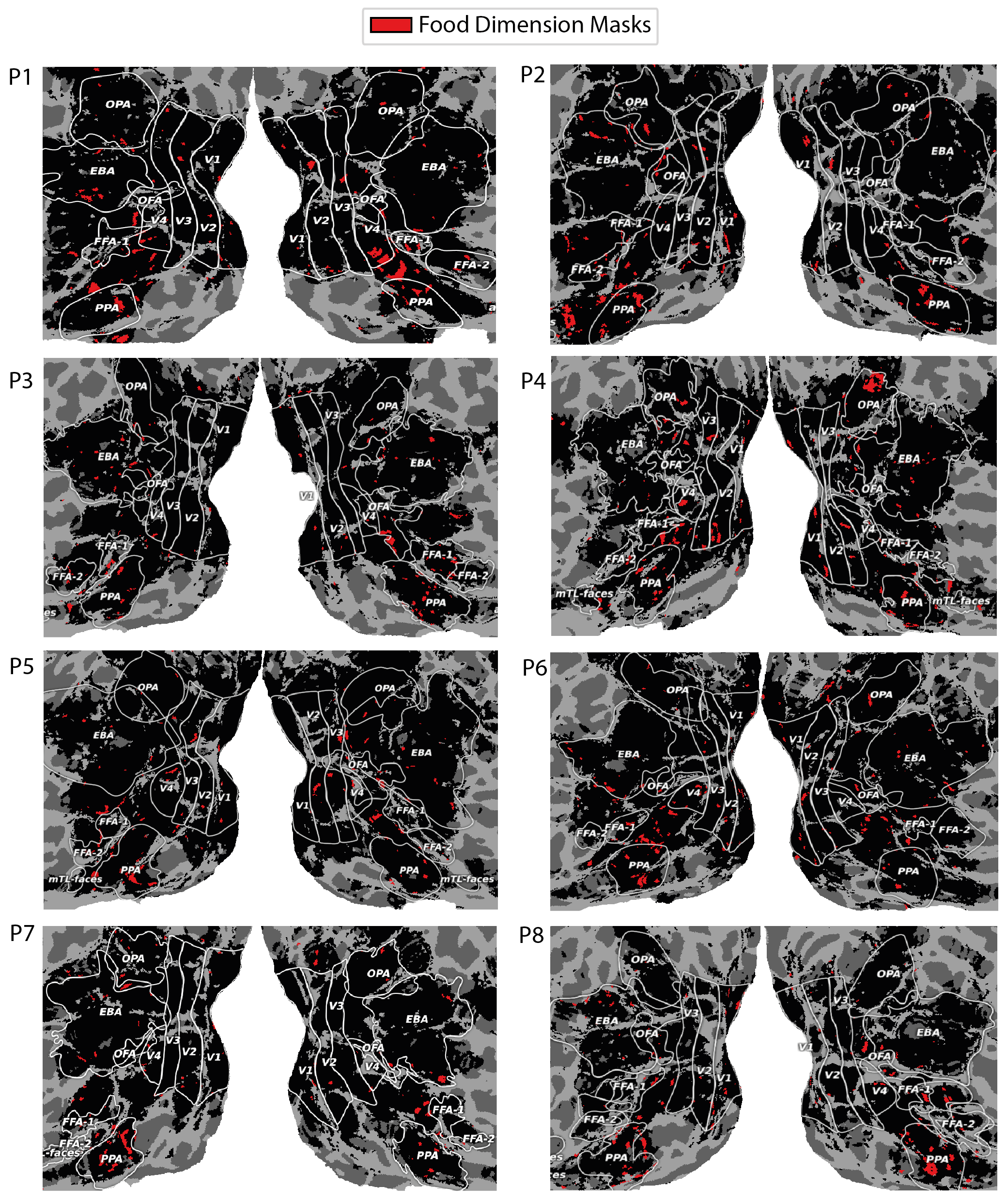
Figure 16 shows a varied set of results across participants. All participants have some level of voxel mask locations in the region between PPA and FFA (inclusive), while most do show a large presence in the regions previously identified as being specific for food. We don’t restrict the area in which the voxel masks are learned and this could lead to some observed differences.