This paper was converted on www.awesomepapers.org from LaTeX by an anonymous user.
Want to know more? Visit the Converter page.

τii+jν¯jντ\tau^{-}\to\ell_{i}^{-}\ell_{i}^{+}\ell_{j}^{-}\bar{\nu}_{j}\nu_{\tau} decays with a magnetic dipole term

M. A. Arroyo-Ureña, E. Díaz, O. Meza-Aldama, G. Tavares-Velasco Facultad de Ciencias Físico-Matemáticas
Benemérita Universidad Autónoma de Puebla, C.P. 72570, Puebla, Pue., Mexico.
(July 28, 2025)
Abstract

Using the massive helicity formalism we calculate the five-body average square amplitude of the decays τii+jν¯jντ\tau^{-}\to\ell_{i}^{-}\ell_{i}^{+}\ell_{j}^{-}\bar{\nu}_{j}\nu_{\tau} (=e,μ)(\ell=e,\,\mu) within the Standard Model (SM), we then introduce a dimension-five effective vertex Γττγ\Gamma^{\tau\tau\gamma} in order to determine the feasibility of imposing limits on the tau anomalous magnetic dipole moment (aτa_{\tau}) via the current or future experimental measurements of the branching ratio for the decay τee+eν¯eντ\tau^{-}\to e^{-}e^{+}e^{-}\bar{\nu}_{e}\nu_{\tau}.

Keywords: tau lepton, magnetic dipole moment, 5-body tau decay, helicity formalism
PACS: 13.35.Dx, 13.40.Em, 12.38.Bx

pacs:
Valid PACS appear here

I Introduction

We found that the SM five body decays τii+jν¯jντ\tau^{-}\to\ell_{i}^{-}\ell_{i}^{+}\ell_{j}^{-}\bar{\nu}_{j}\nu_{\tau} whose branching ratios, at the tree level, have been calculated by Dicus and Vega Dicus , Volobouev of the CLEO Collaboration CLEO and more recently by López Castro et. al. Roig . However Dicus and Roig differ from the predictions of CLEO whose various branching ratios are 7%\sim 7\% higher. The CLEO II experiment has searched for the τee+eνe¯ντ\tau^{-}\to e^{-}e^{+}e^{-}\bar{{\nu}_{e}}\nu_{\tau} decay, whose measured value is PDG :

BR(τee+eνe¯ντ)=2.71.10.40.3+1.5+0.4+0.1×105.BR(\tau^{-}\to e^{-}e^{+}e^{-}\bar{{\nu}_{e}}\nu_{\tau})=2.7^{+1.5+0.4+0.1}_{-1.1-0.4-0.3}\times 10^{-5}. (1)

The statistical, systematic and background uncertainties are 70%\sim 70\% but forthcoming BELLE measurements are expected to improve to 2.7%\sim 2.7\% and 6.5%\sim 6.5\% on the statistical and systematic uncertainties junya , respectively. The importance of our independent calculation is that it is useful to overcome this discrepancy. Furthermore, we analyze the possibility of limiting the aτa_{\tau} value by using current and future experimental measurements by BELLE or other future collaborations.

Leptons offer some of the cleanest signals that can be obtained in collider physics experiments and might also provide new insight into physics beyond the standard model (SM). In particular, with the yet unsolved origin of the discrepancy between the experimental and theoretical SM prediction of the muon anomalous magnetic dipole moment aμa_{\mu}. Although much work has already been devoted to aμa_{\mu}, the aτa_{\tau} has recently become the source of theoretical and experimental interest, which is why in the present work we suggest a tau decay as a means to obtain further insight into aτa_{\tau}. The current lower and upper bounds on aτa_{\tau}, 0.052aτ0.013-0.052\leq a_{\tau}\leq 0.013 with 95%\% C.L. DELPHI , were obtained via the process e+ee+eτ+τe^{+}e^{-}\to e^{+}e^{-}\tau^{+}\tau^{-} by the DELPHI collaboration. These bounds differ from the theoretical value predicted by the SM by one order of magnitude: aτTheor.=1177.21(5)×106a_{\tau}^{\rm Theor.}=1177.21(5)\times 10^{-6} SMMomMagTAU . Measurements of the electron and muon Anomalous Magnetic Dipole Moments (AMDM) were obtained by means of spin precession experiments, however, in the case of the tau lepton this class of measurements are troublesome due to its short lifetime, (290.3±0.5)×1015s(290.3\pm 0.5)\times 10^{-15}s. Even though there is a plethora of tau decays, only a few of them are viable candidates to constrain aτa_{\tau}. Whereas two- and three-body decays do not involve the γττ+\gamma\tau^{-}\tau^{+} coupling, the τ±±ν¯ντγ\tau^{\pm}\to\ell^{\pm}\bar{\nu_{\ell}}\nu_{\tau}\gamma decay, as suggested in Ref. tauTOfourbodies , is constrained by the tau lifetime and is only sensitive to large values of aτa_{\tau}. The use of tau decays to constrain aτa_{\tau} is particularly relevant because the Belle-II experiment is expected to produce about 10910^{9} tau leptons annually, which greatly exceeds the previous CLEO-II experiment, in which there were 3×1063\times 10^{6} produced tau leptons.

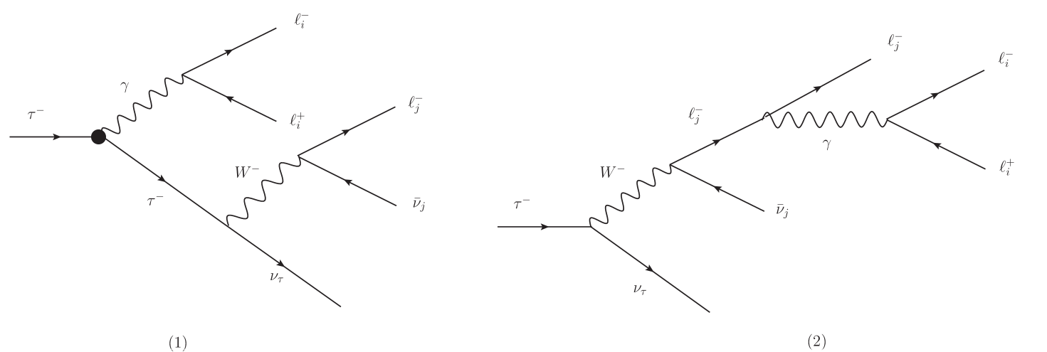
The dominant Feynman diagrams for this decay within the SM are shown in Fig. 1, where the dot represents the QED contribution along with an extra contribution from the tau AMDM. All other tree-level diagrams give a negligible contribution.

In this work we will consider this branching ratio to obtain a bound on aτa_{\tau}. To this aim we will consider the following effective vertex of the photon to a charged lepton pair respecting Lorentz invariance:

Γγ(q)\displaystyle\Gamma^{\gamma\ell\ell}(q) =\displaystyle= ie¯(p2)[FVγγμ+σμνqν(iFMγ+FEγγ5)](p1)Aμ,\displaystyle ie\,\bar{\ell}(p_{2})\left[F_{V}^{\gamma}\gamma^{\mu}+\sigma_{\mu\nu}q^{\nu}\left(iF_{M}^{\gamma}+F_{E}^{\gamma}\gamma_{5}\right)\right]\ell(p_{1})A_{\mu}, (2)

where q=p1p2q=p_{1}-p_{2} is the photon transferred four-momentum. Here FVγ{F_{V}^{\gamma}} is the tau electric charge form factor (FVγ=1{F_{V}^{\gamma}}=1 at the tree level), whereas the five-dimensional CPCP-conserving and CPCP-violating terms correspond to the static anomalous magnetic dipole moment aa_{\ell} and the electric dipole moment dd_{\ell}, which are given by:

aW\displaystyle a_{\ell}^{W} =\displaystyle= 2mFMγ(q2=0),\displaystyle-2m_{\ell}F_{M}^{\gamma}(q^{2}=0), (3)
d\displaystyle d_{\ell} =\displaystyle= eFEγ(q2=0).\displaystyle-eF_{E}^{\gamma}(q^{2}=0). (4)
Refer to caption
Figure 1: Dominant Feynman diagrams in the unitary gauge for the τii+jν¯jντ\tau^{-}\to\ell_{i}^{-}\ell_{i}^{+}\ell_{j}^{-}\bar{\nu}_{j}\nu_{\tau} decay in the SM. The dot represents the QED contribution along with an extra contribution from the tau AMDM. When iji\neq j there are two additional diagrams where the particles with the indices ii and jj are exchanged. Those diagrams will be denoted by the numbers (3) and (4) in our calculation below.

We will assume CPCP invariance and take FEγF_{E}^{\gamma}=0.

The rest of this presentation is organized as follows. In Section II we will present the unpolarized square amplitude for the τee+eν¯eντ\tau^{-}\to e^{-}e^{+}e^{-}\bar{\nu}_{e}\nu_{\tau} decay via the massive helicity formalism dittmaier , which considerably simplifies the calculation. The numerical integration of the τee+eν¯eντ\tau^{-}\to e^{-}e^{+}e^{-}\bar{\nu}_{e}\nu_{\tau} decay width and the resulting bound on the aτa_{\tau} are presented in Sec. III, whereas Sec. IV is devoted to the conclusions and outlook. Details of the calculation are presented in Appendix A.

II Unpolarized square amplitude

We will calculate the average square amplitude of the τii+jν¯jντ\tau^{-}\to\ell_{i}^{-}\ell_{i}^{+}\ell_{j}^{-}\bar{\nu}_{j}\nu_{\tau} decay using the massive helicity formalism for which usual treatments, such as dixon or elvang , only deal with the massless case. Here we need to take into account the mass of the tau lepton, so must go further. In particular, in dittmaier the two main ways to deal with massive helicity amplitudes are presented, although with a somewhat old-fashioned notation. We use here the approach that consists in performing a light-cone decomposition to write the four-momentum of a massive particle as a linear combination of two light-like momenta. For a detail account we refer the interested reader to Ref. proceedings , where this formalism is presented in a self-contained manner (with opposite metric signature convention). We will present a brief outline here for convenience.

Let pp be the four-momentum of a massive particle of mass m>0m>0, which can always be written in terms of two light-like ones qμq^{\mu} and rμr^{\mu} as

pμ=rμ+m22pqqμ,p^{\mu}=r^{\mu}+\frac{m^{2}}{2p\cdot q}q^{\mu}, (5)

where qq satisfies pq0p\cdot q\neq 0 but is otherwise arbitrary, and rr is defined through (5). The positive frequency momentum space Dirac equation has two linearly independent solutions, which we label with the subindices ++ and -. It is easily checked that they are given (maybe up to a phase) by

u+=|r+m[rq]|q],u=|r]+mrq|q;u_{+}=|r\rangle+\frac{m}{[rq]}|q]\quad,\quad u_{-}=|r]+\frac{m}{\langle rq\rangle}|q\rangle; (6)

while for the negative frequency we have

v+=|r]+mqr|q,v=|r+m[qr]|q].v_{+}=|r]+\frac{m}{\langle qr\rangle}|q\rangle\quad,\quad v_{-}=|r\rangle+\frac{m}{[qr]}|q]. (7)

Here |a]|a] and |b|b\rangle are 2-component Weyl spinors linked to the light-like momenta aμa_{\mu} and bμb_{\mu} proceedings . We will use these solutions to calculate the helicity amplitudes ah1h2h3h4h5h6\mathcal{M}_{a}^{h_{1}h_{2}h_{3}h_{4}h_{5}h_{6}} for the τ(p1)i(p2)i+(p3)j(p4)ν¯j(p5)ντ(p6)\tau^{-}(p_{1})\to\ell_{i}^{-}(p_{2})\ell_{i}^{+}(p_{3})\ell_{j}^{-}(p_{4})\bar{\nu}_{j}(p_{5})\nu_{\tau}(p_{6}) decay, where hkh_{k} is the helicity of the particle kk with four-momentum pkp_{k}, and the subindex aa labels each Feynman diagram of Fig. 1: it runs from 1 to 4 in the case that the charged leptons i\ell_{i}^{-} and j\ell_{j}^{-} are identical, such as in the τee+eν¯eντ\tau^{-}\to e^{-}e^{+}e^{-}\bar{\nu}_{e}\nu_{\tau} decay, but it only runs from from 1 to 2 if i\ell_{i}^{-} and j\ell_{j}^{-} are distinguishable.

To determine the individual non-zero helicity amplitudes we will neglect the mass of the outgoing charged leptons, which is a good approximation as their mass is negligible as compared to the tau mass. In this limit, each amplitude will vanish unless the helicities of particles 4, 5 and 6 have certain fixed signs because of its spinor index structure. After doing that, we present the sum of the squared modulus of the helicity amplitudes and then all of the interferences.

In the unitary gauge, the amplitude for the first Feynman diagram of Fig. 1, dubbed (1), is

1\displaystyle\mathcal{M}_{1} =\displaystyle= G1u¯(4)γμPLv(5)(gμνk3μk3νmW2)u¯(6)γνPL(2+mτ)(γρFVγ+iσρβk1βFMγ)u(1)\displaystyle G_{1}\bar{u}(4)\gamma^{\mu}P_{L}v(5)\left(g_{\mu\nu}-\frac{{k_{3}}_{\mu}{k_{3}}_{\nu}}{m_{W}^{2}}\right)\bar{u}(6)\gamma^{\nu}P_{L}(\not{k}_{2}+m_{\tau})(\gamma^{\rho}{F_{V}^{\gamma}}+i\sigma^{\rho\beta}{k_{1}}_{\beta}F_{M}^{\gamma})u(1) (8)
×\displaystyle\times u¯(2)γλv(3),\displaystyle\bar{u}(2)\gamma_{\lambda}v(3),

where we use the short-hand notation (i)(pi)(i)\equiv(p_{i}) and the four-momenta kik_{i} are the ones of the virtual particles of this diagram. Note that we are using the effective interaction (2) for the γτ¯τ\gamma\bar{\tau}\tau vertex but in our calculation below we will use the tree-level value FVγ=1F_{V}^{\gamma}=1. In addition

G1gW2e28p23(p23p12p13)(2p45mW2),G_{1}\equiv\frac{g_{W}^{2}e^{2}}{8p_{23}(p_{23}-p_{12}-p_{13})(2p_{45}-m_{W}^{2})}, (9)

with pij=pipjp_{ij}=p_{i}\cdot p_{j}. The helicity structure of the amplitude fixes h4=h_{4}=-, h5=+h_{5}=+, and h6=h_{6}=-. We then write

1=G14|γμ|5]6|γμ(2+mτ)γν(FVγFMγ1)u(1)u¯(2)γνv(3).\mathcal{M}_{1}=G_{1}\langle 4|\gamma_{\mu}|5]\langle 6|\gamma^{\mu}(\not{k}_{2}+m_{\tau})\gamma^{\nu}\left({F_{V}^{\gamma}}-{F_{M}^{\gamma}}\not{k}_{1}\right)u(1)\bar{u}(2)\gamma_{\nu}v(3). (10)

We now choose q1p3q_{1}\equiv p_{3} and define

D1p13p23FVγmτFMγ,\displaystyle D_{1}\equiv\frac{p_{13}}{p_{23}}{F_{V}^{\gamma}}-m_{\tau}{F_{M}^{\gamma}}, (11)
EmτFVγ2p13FMγ,\displaystyle E\equiv m_{\tau}{F_{V}^{\gamma}}-2p_{13}{F_{M}^{\gamma}}, (12)

thus the individual helicity amplitudes are given by

1+++=4G164[23][r3](E([54]43+[56]63)mτD132[25]),\mathcal{M}_{1}^{++--+-}=4G_{1}\frac{\langle 64\rangle[23]}{[r3]}\left(E([54]\langle 43\rangle+[56]\langle 63\rangle)-m_{\tau}D_{1}\langle 32\rangle[25]\right), (13)
1+++=4G164r2(mτFVγ[35]FMγ[23]([54]42+[56]62)),\mathcal{M}_{1}^{+-+-+-}=4G_{1}\langle 64\rangle\langle r2\rangle\left(m_{\tau}{F_{V}^{\gamma}}[35]-{F_{M}^{\gamma}}[23]([54]\langle 42\rangle+[56]\langle 62\rangle)\right), (14)
1++=4G164[2r](FVγ([54]43+[56]63)+mτFMγ32[25]),\mathcal{M}_{1}^{-+--+-}=4G_{1}\langle 64\rangle[2r]\left({F_{V}^{\gamma}}([54]\langle 43\rangle+[56]\langle 63\rangle)+m_{\tau}{F_{M}^{\gamma}}\langle 32\rangle[25]\right), (15)

and

1++=4G164r3(2p23D1([54]42+[56]62)mτE23[35]).\mathcal{M}_{1}^{--+-+-}=4G_{1}\frac{\langle 64\rangle}{\langle r3\rangle}\left(2p_{23}D_{1}([54]\langle 42\rangle+[56]\langle 62\rangle)-m_{\tau}E\langle 23\rangle[35]\right). (16)

To obtain the helicity amplitudes of the the third Feynman diagram, obtained from the first one after the exchange of identical particles, we simply exchange the momenta and helicities of particles 2 and 4, both in the helicity amplitudes and in the definitions of D1D_{1} and G1G_{1}, leading to new coefficients that we denote as D3D_{3} and G3G_{3}, respectively.

By an analogous procedure, we obtain for the Feynman diagram (2) of Fig. 1

2+++=4mτH2[53]34[r3](63[32]+64[42]),\displaystyle\mathcal{M}_{2}^{++--+-}=4m_{\tau}H_{2}\frac{[53]\langle 34\rangle}{[r3]}(\langle 63\rangle[32]+\langle 64\rangle[42]), (17)
2+++=4mτH224[53][r3](62[23]+64[43]),\displaystyle\mathcal{M}_{2}^{+-+-+-}=4m_{\tau}H_{2}\frac{\langle 24\rangle[53]}{[r3]}(\langle 62\rangle[23]+\langle 64\rangle[43]), (18)
2++=4H234[5r](63[32]+64[42]),\displaystyle\mathcal{M}_{2}^{-+--+-}=4H_{2}\langle 34\rangle[5r](\langle 63\rangle[32]+\langle 64\rangle[42]), (19)
2++=4H224[5r](62[23]+64[43]);\displaystyle\mathcal{M}_{2}^{--+-+-}=4H_{2}\langle 24\rangle[5r](\langle 62\rangle[23]+\langle 64\rangle[43]); (20)

where

H2gW2e28p23(p23+p24+p34)(mτ2mW2p16).H_{2}\equiv\frac{g_{W}^{2}e^{2}}{8p_{23}\left(p_{23}+p_{24}+p_{34}\right)\left(m_{\tau}^{2}-m_{W}^{2}-p_{16}\right)}. (21)

We straightforwardly obtain the corresponding amplitudes for the fourth diagram after the exchange of the momenta and helicities of particles 2 and 4.

We now factor all the dependence on the form factors FVγ{F_{V}^{\gamma}} and FMγ{F_{M}^{\gamma}} by defining the following coefficients:

A12p12FVγ2+p23p13(E2+mτ2FVγ2),\displaystyle A_{1}\equiv 2p_{12}{F_{V}^{\gamma}}^{2}+\frac{p_{23}}{p_{13}}(E^{2}+m_{\tau}^{2}{F_{V}^{\gamma}}^{2}), (22)
B12p12FMγ2+p23p13(D12+mτ2FMγ2),\displaystyle B_{1}\equiv 2p_{12}{F_{M}^{\gamma}}^{2}+\frac{p_{23}}{p_{13}}(D_{1}^{2}+m_{\tau}^{2}{F_{M}^{\gamma}}^{2}), (23)
C12p12FVγFMγ+p23p13(mτ2FVγFMD1E),\displaystyle C_{1}\equiv 2p_{12}{F_{V}^{\gamma}}{F_{M}^{\gamma}}+\frac{p_{23}}{p_{13}}(m_{\tau}^{2}{F_{V}^{\gamma}}F_{M}-D_{1}E), (24)

from which we obtain the sum of the squared helicity amplitudes of the first diagram:

h|1|2\displaystyle\sum_{h}\left|\mathcal{M}_{1}\right|^{2} =128G12p46[A1(mτ22p35+p34p45+p36p56+p3456)\displaystyle=128G_{1}^{2}p_{46}\Bigg{[}A_{1}\left(\frac{m_{\tau}^{2}}{2}p_{35}+p_{34}p_{45}+p_{36}p_{56}+p_{3456}\right)
+2p23B1(mτ22p25+p25p45+p26p56+p2654)+2mτp23C1(p45+p56)],\displaystyle+2p_{23}B_{1}\left(\frac{m_{\tau}^{2}}{2}p_{25}+p_{25}p_{45}+p_{26}p_{56}+p_{2654}\right)+2m_{\tau}p_{23}C_{1}(p_{45}+p_{56})\Bigg{]}, (25)

where pi1i2iNp_{i_{1}i_{2}\cdots i_{N}} is defined in Appendix A. For the second diagram we get

h|2|2\displaystyle\sum_{h}\left|\mathcal{M}_{2}\right|^{2} =256H22(mτ2p35p13+p15)[p24(p23p26+p34p46+p3264)\displaystyle=256H_{2}^{2}\left(m_{\tau}^{2}\frac{p_{35}}{p_{13}}+p_{15}\right)\left[p_{24}(p_{23}p_{26}+p_{34}p_{46}+p_{3264})\right.
+p34(p23p36+p24p46+p2364)].\displaystyle\left.+p_{34}(p_{23}p_{36}+p_{24}p_{46}+p_{2364})\right]. (26)

The corresponding expression for the fourth diagram is attained by exchanging p2p_{2} and p4p_{4}.

On the other hand, the non-zero interferences are given by

12=64G1H2[2FVγ(𝒬12(0)+mτ2p13𝒬12(2))mτFMγ12(0)],\mathcal{I}_{12}=64G_{1}H_{2}\left[2{F_{V}^{\gamma}}\left(\mathcal{Q}^{(0)}_{12}+\frac{m_{\tau}^{2}}{p_{13}}\mathcal{Q}^{(2)}_{12}\right)-m_{\tau}{F_{M}^{\gamma}}\mathcal{R}^{(0)}_{12}\right], (27)
13\displaystyle\mathcal{I}_{13} =64G1G3[FVγ2(p13𝒬13(0)+mτ2𝒬13(2)+m4p13𝒬13(4))+2FMγ2(13(0)+mτ213(2))\displaystyle=64G_{1}G_{3}\Bigg{[}{F_{V}^{\gamma}}^{2}\left(p_{13}\mathcal{Q}^{(0)}_{13}+m_{\tau}^{2}\mathcal{Q}^{(2)}_{13}+\frac{m^{4}}{p_{13}}\mathcal{Q}^{(4)}_{13}\right)+2{F_{M}^{\gamma}}^{2}\left(\mathcal{R}^{(0)}_{13}+m_{\tau}^{2}\mathcal{R}^{(2)}_{13}\right)
mτFVγFMγ(𝒫13(0)+mτ2𝒫13(2))],\displaystyle-m_{\tau}{F_{V}^{\gamma}}{F_{M}^{\gamma}}\left(\mathcal{P}^{(0)}_{13}+m_{\tau}^{2}\mathcal{P}^{(2)}_{13}\right)\Bigg{]}, (28)
14=64G1H4[2FVγ(𝒬14(0)+mτ2p13𝒬14(2))+mτFMγ14(0)],\mathcal{I}_{14}=64G_{1}H_{4}\left[2{F_{V}^{\gamma}}\left(\mathcal{Q}^{(0)}_{14}+\frac{m_{\tau}^{2}}{p_{13}}\mathcal{Q}^{(2)}_{14}\right)+m_{\tau}{F_{M}^{\gamma}}\mathcal{R}^{(0)}_{14}\right], (29)

and

24=512H2H4p15p24(p23p26+p34p46+p2346);\mathcal{I}_{24}=-512H_{2}H_{4}p_{15}p_{24}\left(p_{23}p_{26}+p_{34}p_{46}+p_{2346}\right); (30)

where ij\mathcal{I}_{ij} stands for the interference between the amplitudes of diagrams ii and jj. Explicit expressions for the (𝒫,𝒬,)ij(p)\left(\mathcal{P},\mathcal{Q},\mathcal{R}\right)^{(p)}_{ij} functions are given in Appendix A.

The full unpolarized squared amplitude for the τee+eν¯eντ\tau^{-}\to e^{-}e^{+}e^{-}\bar{\nu}_{e}\nu_{\tau} decay is given by

|¯|2=12(i=14h|i|2+12+13+14+24),|\overline{\mathcal{M}}|^{2}=\frac{1}{2}\left(\sum_{i=1}^{4}\sum_{h}\left|\mathcal{M}_{i}\right|^{2}+\mathcal{I}_{12}+\mathcal{I}_{13}+\mathcal{I}_{14}+\mathcal{I}_{24}\right), (31)

It is worth noting that this method is straightforward and yields compact results easy to handle in the numerical integration.

III Numerical results

We now turn to compute the branching ratio of the tau five-body decay τee+eν¯eντ\tau^{-}\to e^{-}e^{+}e^{-}\bar{\nu}_{e}\nu_{\tau}. The decay width is given by the usual formula

Γ(τee+eν¯eντ)=(2π)42mτi=15d3pi16π3Ei|¯|2δ4(p1i=26pi).\Gamma(\tau^{-}\to e^{-}e^{+}e^{-}\bar{\nu}_{e}\nu_{\tau})=\frac{(2\pi)^{4}}{2m_{\tau}}\int\prod_{i=1}^{5}\frac{d^{3}p_{i}}{16\pi^{3}E_{i}}|\overline{\mathcal{M}}|^{2}\delta^{4}\left(p_{1}-\sum_{i=2}^{6}p_{i}\right). (32)

After dividing by the tau total width Γτ=1/ττ\Gamma_{\tau}=1/\tau_{\tau} we obtain the corresponding branching ratio

BR(τee+eν¯eντ)=Γ(τee+eν¯eντ)Γτ.BR(\tau^{-}\to e^{-}e^{+}e^{-}\bar{\nu}_{e}\nu_{\tau})=\frac{\Gamma(\tau^{-}\to e^{-}e^{+}e^{-}\bar{\nu}_{e}\nu_{\tau})}{\Gamma_{\tau}}. (33)

According to Ref.EspFase the four-momenta of the involved particles in a five-body decay can be related to eight independent Lorentz invariant parameters through the relations:

s1=(p1p4)2,s2=(p1p4p2)2,s3=(p1p4p2p3)2,s_{1}=(p_{1}-p_{4})^{2},\,s_{2}=(p_{1}-p_{4}-p_{2})^{2},\,s_{3}=(p_{1}-p_{4}-p_{2}-p_{3})^{2}, (34)
u1=(p1p2)2,u2=(p1p3)2,u3=(p1p5)2,u_{1}=(p_{1}-p_{2})^{2},\,u_{2}=(p_{1}-p_{3})^{2},\,u_{3}=(p_{1}-p_{5})^{2}, (35)
t2=(p1p2p3)2,t3=(p1p2p3p5)2.t_{2}=(p_{1}-p_{2}-p_{3})^{2},\,t_{3}=(p_{1}-p_{2}-p_{3}-p_{5})^{2}. (36)

The phase-space integral (32) was numerically computed over these kinematic variables via Monte-Carlo integration by using the VEGAS routines Lepage . A cross-check of our results was done by implementing the electromagnetic vertex in the CalcHEP package Belyaev:2012qa , which performs all the numerical calculation.

We first consider that the impact of the magnetic form factor is negligible, i.e. we use FMγ=0F_{M}^{\gamma}=0 and make a comparison of our numerical results for the widths of the allowed τij+iν¯jντ\tau^{-}\to\ell_{i}^{-}\ell_{j}^{+}\ell_{i}^{-}\bar{{\nu}_{\ell}}_{j}\nu_{\tau} decays with those obtained in previous studies. The results are shown in Table 1. The uncertainties arise from the numerical integration. Our results are in good agreement with these predictions, though are closer to those of Ref. Roig , which could be attributed to the fact that we used the same values of the tau mass and mean lifetime. Additionally, for completeness, we computed the μee+eνe¯νμ\mu^{-}\to e^{-}e^{+}e^{-}\bar{\nu_{e}}\nu_{\mu} for which we obtain BR(μee+eνe¯νμ)=(3.599±0.002)×105BR(\mu^{-}\to e^{-}e^{+}e^{-}\bar{\nu_{e}}\nu_{\mu})=(3.599\pm 0.002)\times 10^{-5}.

Branching ratio RefDicus Ref. CLEO Ref. Roig Our results
BR(τee+eνe¯ντ)105\frac{BR(\tau^{-}\to e^{-}e^{+}e^{-}\bar{\nu_{e}}\nu_{\tau})}{10^{-5}} 4.15±0.064.15\pm 0.06 4.457±0.0064.457\pm 0.006 4.21±0.014.21\pm 0.01 4.22±0.024.22\pm 0.02
BR(τeμ+μνe¯ντ)107\frac{BR(\tau^{-}\to e^{-}\mu^{+}\mu^{-}\bar{\nu_{e}}\nu_{\tau})}{10^{-7}} 1.257±0.0031.257\pm 0.003 1.347±0.0021.347\pm 0.002 1.247±0.0011.247\pm 0.001 1.246±0.0021.246\pm 0.002
BR(τμe+eνμ¯ντ)105\frac{BR(\tau^{-}\to\mu^{-}e^{+}e^{-}\bar{\nu_{\mu}}\nu_{\tau})}{10^{-5}} 1.97±0.021.97\pm 0.02 2.089±0.0032.089\pm 0.003 1.984±0.0041.984\pm 0.004 1.987±0.0031.987\pm 0.003
BR(τμμ+μνμ¯ντ)107\frac{BR(\tau^{-}\to\mu^{-}\mu^{+}\mu^{-}\bar{\nu_{\mu}}\nu_{\tau})}{10^{-7}} 1.190±0.0021.190\pm 0.002 1.276±0.0051.276\pm 0.005 1.183±0.0011.183\pm 0.001 1.184±0.0011.184\pm 0.001
Table 1: Branching ratios for the allowed τij+iν¯jντ\tau^{-}\to\ell_{i}^{-}\ell_{j}^{+}\ell_{i}^{-}\bar{{\nu}_{\ell}}_{j}\nu_{\tau} decays in the SM.

III.1 Effect of FMγF_{M}^{\gamma} on the τee+eνe¯ντ\tau^{-}\to e^{-}e^{+}e^{-}\bar{\nu_{e}}\nu_{\tau} decay

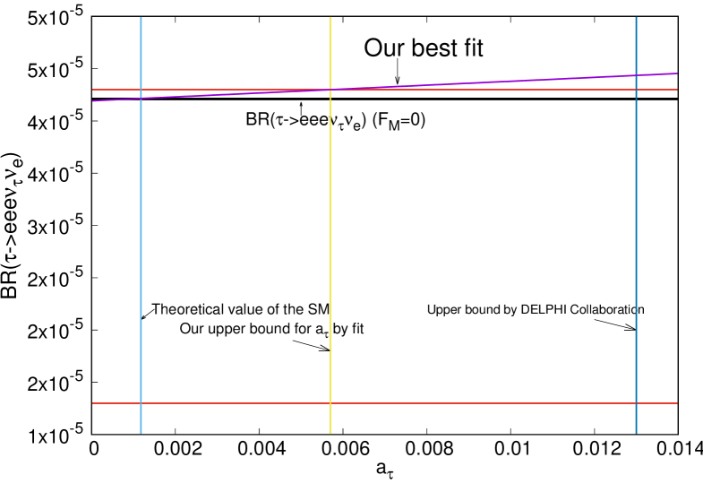
We will now analyze the impact of the dipole term FMγF_{M}^{\gamma} on the branching ratio of the tau five-body decay. The behavior of BR(τee+eνe¯ντ)BR(\tau^{-}\to e^{-}e^{+}e^{-}\bar{\nu_{e}}\nu_{\tau}) as a function of aτa_{\tau} is shown in Fig. 2. The horizontal red lines corresponds to the 95% C.L. interval obtained from the experimental measurement of BR(τee+eνe¯ντ)BR(\tau^{-}\to e^{-}e^{+}e^{-}\bar{{\nu}_{e}}\nu_{\tau}) PDG , and the horizontal black line corresponds to our calculation for the tree-level SM prediction, i.e. BR(τee+eνe¯ντ)=(4.22±0.02)×105BR(\tau^{-}\to e^{-}e^{+}e^{-}\bar{{\nu}_{e}}\nu_{\tau})=(4.22\pm 0.02)\times 10^{-5}. The purple curve corresponds to our prediction for the branching ratio as a function of aτa_{\tau}. Assuming that there are no extra contribution rather than that due to aτa_{\tau} we can conclude that the points of the purple curve falling above the upper experimental bound on BR(τee+eνe¯ντ)BR(\tau^{-}\to e^{-}e^{+}e^{-}\bar{{\nu}_{e}}\nu_{\tau}) would be excluded, thereby yielding the bound aτ0.0056a_{\tau}\leq 0.0056. This allow us to gain an improvement over the current upper bound by DELPHI: aτDELPHI0.013a_{\tau}^{\rm DELPHI}\leq 0.013. Since there is a slight dependence of BR(τee+eνe¯ντ)BR(\tau^{-}\to e^{-}e^{+}e^{-}\bar{{\nu}_{e}}\nu_{\tau}) on aτa_{\tau}, this method is not useful to set a lower bound on it with current measurements.

Refer to caption
Figure 2: BR(τee+eνe¯ντ)BR(\tau^{-}\to e^{-}e^{+}e^{-}\bar{{\nu}_{e}}\nu_{\tau}) as a function of aτa_{\tau} (purple line). The horizontal red lines are the 95% C.L. limits on the experimental measurement of the five-body decay, of which the central value is 2.7×1052.7\times 10^{-5}. Whereas the horizontal black line is the tree-level SM prediction (FM=0F_{M}=0). On the other hand, the vertical lines are the SM prediction of aτa_{\tau}(blue line), our bound (yellow line), and the upper DELPHI bound (dark blue line).

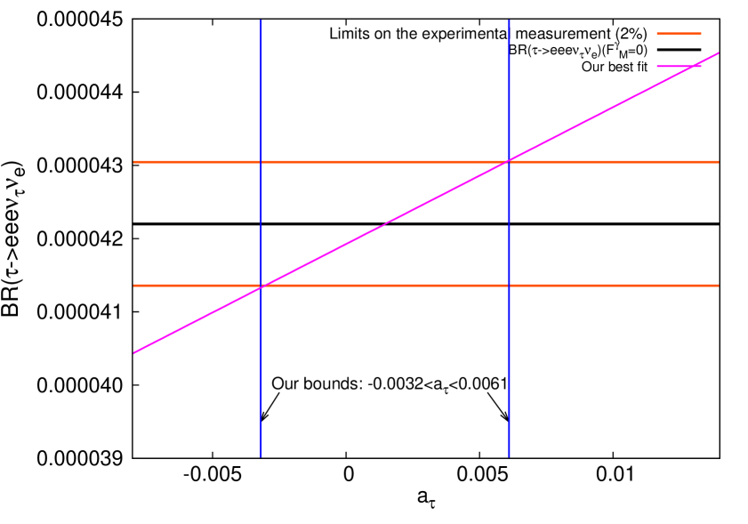
Forthcoming measurements might reach a statistical uncertainty of 2.7%2.7\% and a systematic uncertainty of 6.5%6.5\%. Which we found is not good enough so that we may obtain improved bounds, since our lower bound would only improve to a level of \sim-0.02. But new runs at BELLE II or future experiments we hope might offer more precise measurements, which is why we optimistically assume that if the statistical and systematic uncertainty is improved to the 2% level, we expect to find that the bound of aτa_{\tau} would fall in the range of 0.0032aτ0.0061-0.0032\leq a_{\tau}\leq 0.0061, see Fig. 3.

Refer to caption
Figure 3: With an improvement of the uncertainties at the 2% level in BR(τee+eνe¯ντ)BR(\tau^{-}\to e^{-}e^{+}e^{-}\bar{{\nu}_{e}}\nu_{\tau}), our best fit prediction of aτa_{\tau} (purple line), along with the improved measurements (red lines) allow us to ascertain that 0.0032aτ0.0061-0.0032\leq a_{\tau}\leq 0.0061. The horizontal black line is the tree-level SM prediction (FM=0F_{M}=0).

Other approaches similarly yield stringent bounds on aτa_{\tau} through electroweak precision data (EWPD) and the experimental data for the e+eτ+τe^{+}e^{-}\to\tau^{+}\tau^{-}: 0.004aτ0.006-0.004\leq a_{\tau}\leq 0.006 Escribano , 0.007aτ0.005-0.007\leq a_{\tau}\leq 0.005 Springberg and more recently 0.007aτ0.004-0.007\leq a_{\tau}\leq 0.004 Epifanov . While on the theoretical side, other model extensions predict values for aτa_{\tau} of the order of 𝒪(109106)\mathcal{O}(10^{-9}-10^{-6}) MoyTav -MSSM , which could be useful in the case of a discrepancy between the experimental measurement and the SM prediction.

IV Conclusions

In this work we present the results of a numerical calculation for the predictions of the branching ratio of the allowed τii+jν¯jντ\tau^{-}\to\ell_{i}^{-}\ell_{i}^{+}\ell_{j}^{-}\bar{\nu}_{j}\nu_{\tau} decays, which are consistent with previous results reported by Dicus and Vega and López Castro et. al. In addition, we use the current experimental measurement on the branching ratio of the τee+eνe¯ντ\tau^{-}\to e^{-}e^{+}e^{-}\bar{{\nu}_{e}}\nu_{\tau} decay to obtain an upper limit on the tau anomalous magnetic dipole moment by using an effective electromagnetic vertex including a dipole term. We find that the effect of the magnetic dipole form factor FMγF_{M}^{\gamma} on the reported value by CLEO II colaboration for the branching ratio of the τee+eνe¯ντ\tau^{-}\to e^{-}e^{+}e^{-}\bar{{\nu}_{e}}\nu_{\tau} decay allows to extract an upper bound of aτ0.0056a_{\tau}\leq 0.0056, which is below the current upper bound by the DELPHI collaboration. With the next measurements by BELLE II results are expected with 2.7%\sim 2.7\% and 6.5%\sim 6.5\% of statistical and systematic uncertainties. Under this scenario, we find that the effect of FMγF_{M}^{\gamma} on the BR(τe+e+eν¯eντ)BR(\tau^{-}\to e^{+}e^{+}e^{-}\bar{\nu}_{e}\nu_{\tau}) is such that the lower bound is given by 0.02aτ-0.02\leq a_{\tau} but it is not possible to extract a good upper bound. Finally, assuming an accurate measurement of the 2%2\% of statistical and systematic uncertainties, it is found that our best bounds are 0.0032aτ0.0061-0.0032\leq a_{\tau}\leq 0.0061.

Acknowledgements.
We acknowledge support from CONACYT (México).

Appendix A Conventions for the massive helicity formalism and interference terms for the τee+eνe¯ντ\tau^{-}\to e^{-}e^{+}e^{-}\bar{{\nu}_{e}}\nu_{\tau} unpolarized square amplitude.

We use the abbreviated notation

pi1i2iN12Re([i1i2]i2i3[iN1iN]iNi1)p_{i_{1}i_{2}\dots i_{N}}\equiv\frac{1}{2}\text{Re}\left([i_{1}i_{2}]\langle i_{2}i_{3}\rangle\dots[i_{N-1}i_{N}]\langle i_{N}i_{1}\rangle\right) (37)

(where Re(z)\text{Re}(z) stands for the real part of the complex number zz), with NN even. It is easy to show that

pi1i2iN=14i1μ1i2μ2iNTrμN(γμ1γμ2γμN).p_{i_{1}i_{2}\dots i_{N}}=\frac{1}{4}{i_{1}}_{\mu_{1}}{i_{2}}_{\mu_{2}}\dots i_{N}{}_{\mu_{N}}\text{Tr}\left(\gamma^{\mu_{1}}\gamma^{\mu_{2}}\dots\gamma^{\mu_{N}}\right). (38)

It is well known that, for NN even, the trace of the product of NN gamma matrices is proportional (the proportionality constant being 44) to (N1)!!(N-1)!! terms, each of which is the product of N/2N/2 metric tensors. In the particular case of only two indices we write pabp_{ab} as an abbreviation of papbp_{a}\cdot p_{b} even when the momenta pap_{a} and pbp_{b} are not null. When there are more indices the individual momenta must be light-like.
Several properties can be obtained immediately. For instance, cyclicity of the trace translates into cyclicity of indices:

pi1i2iN1iN=piNi1i2iN1.p_{i_{1}i_{2}\dots i_{N-1}i_{N}}=p_{i_{N}i_{1}i_{2}\dots i_{N-1}}. (39)

Using the definition (37) we see that a multi-index pp with two equal adjacent indices vanishes because

[pp]=pp=0.[pp]=\langle pp\rangle=0. (40)

On the other hand, using {γμ,γν}=2gμν\{\gamma^{\mu},\gamma^{\nu}\}=2g^{\mu\nu} we obtain the following general “index-commuting formula”:

pi1i2ik1ikik+1ik+2iN=2pikik+1pi1i2ik1ik+2iNpi1i2ik1ik+1ikik+2iN.p_{i_{1}i_{2}\dots i_{k-1}i_{k}i_{k+1}i_{k+2}\dots i_{N}}=2p_{i_{k}i_{k+1}}p_{i_{1}i_{2}\dots i_{k-1}i_{k+2}\dots i_{N}}-p_{i_{1}i_{2}\dots i_{k-1}i_{k+1}i_{k}i_{k+2}\dots i_{N}}. (41)

In a scattering (or decay) process with LL external legs, we have LL distinct four-momenta. If we calculate a squared amplitude and get a pp with more than LL indices, we use the (40) and (41) properties to write everything in terms of only pp’s with at most LL indices, i.e. LL is an upper bound for the number of indices in an LL particle tree level process. In our case there are six external legs, therefore pp’s with more than six indices shall not appear.
For the interferences we use the following expressions:

𝒬12(0)\displaystyle\mathcal{Q}^{(0)}_{12} =p24(2p46p3r54+p2645r3)+p34(2p46p2r54+p2r5463)\displaystyle=p_{24}\left(2p_{46}p_{3r54}+p_{2645r3}\right)+p_{34}\left(2p_{46}p_{2r54}+p_{2r5463}\right) (42)
+p46(p2r5634+p243r56)p26p2465r3p36p2r5643,\displaystyle+p_{46}\left(p_{2r5634}+p_{243r56}\right)-p_{26}p_{2465r3}-p_{36}p_{2r5643}, (43)
𝒬12(2)=\displaystyle\mathcal{Q}^{(2)}_{12}= 2p35p46p243r+p23(p34p3645p36p3564)+p46(p34p2354p36p2534+p35p2634)\displaystyle 2p_{35}p_{46}p_{243r}+p_{23}\left(p_{34}p_{3645}-p_{36}p_{3564}\right)+p_{46}\left(p_{34}p_{2354}-p_{36}p_{2534}+p_{35}p_{2634}\right) (44)
+\displaystyle+ p13(p26p2534+p34p2563+p46p2534p24p2536p36p2543p46p2453),\displaystyle p_{13}\left(p_{26}p_{2534}+p_{34}p_{2563}+p_{46}p_{2534}-p_{24}p_{2536}-p_{36}p_{2543}-p_{46}p_{2453}\right), (45)
12(0)=4\displaystyle\mathcal{R}^{(0)}_{12}=4 [p23(p34p3645p36p3564)+p46(p34p2354p36p2534p35p2634)\displaystyle\Big{[}p_{23}(p_{34}p_{3645}-p_{36}p_{3564})+p_{46}(p_{34}p_{2354}-p_{36}p_{2534}p_{35}p_{2634}) (46)
+p35(p46p24r3p26p2r34+p24p2r36)p13(p24p2536p26p2534+p46p2453)\displaystyle+p_{35}(p_{46}p_{24r3}-p_{26}p_{2r34}+p_{24}p_{2r36})-p_{13}(p_{24}p_{2536}-p_{26}p_{2534}+p_{46}p_{2453}) (47)
+p12(p46p2435p34p2635+p36p2435)p25(p46p243rp34p263r+p36p243r)\displaystyle+p_{12}(p_{46}p_{2435}-p_{34}p_{2635}+p_{36}p_{2435})-p_{25}(p_{46}p_{243r}-p_{34}p_{263r}+p_{36}p_{243r}) (48)
p24p46p13(p13p2653p34p253r+p35p243r2p23p3r54)\displaystyle-\frac{p_{24}p_{46}}{p_{13}}\left(p_{13}p_{2653}-p_{34}p_{253r}+p_{35}p_{243r}-2p_{23}p_{3r54}\right) (49)
+p23(p24p2645p26p2465+p46p2456)];\displaystyle+p_{23}\left(p_{24}p_{2645}-p_{26}p_{2465}+p_{46}p_{2456}\right)\Big{]}; (50)
𝒬13(0)=4(2p26p46p56+p46p2654p24p2645+p26p2465),\mathcal{Q}^{(0)}_{13}=4\left(2p_{26}p_{46}p_{56}+p_{46}p_{2654}-p_{24}p_{2645}+p_{26}p_{2465}\right), (51)
𝒬13(2)=2\displaystyle\mathcal{Q}^{(2)}_{13}=2 (p35p264r+p45p2634p34p2654p26p3465+p24p6253p46p2653p26p4253),\displaystyle\left(p_{35}p_{264r}+p_{45}p_{2634}-p_{34}p_{2654}-p_{26}p_{3465}+p_{24}p_{6253}-p_{46}p_{2653}-p_{26}p_{4253}\right), (52)
𝒬13(4)=p35p2643,\mathcal{Q}^{(4)}_{13}=p_{35}p_{2643}, (53)
13(0)\displaystyle\mathcal{R}^{(0)}_{13} =4p26(p46p56p234r+p23p46p254rp23p45p264r)4p24(p23p45p264rp25p46p324r+p23p46p524r)\displaystyle=4p_{26}\left(p_{46}p_{56}p_{234r}+p_{23}p_{46}p_{254r}-p_{23}p_{45}p_{264r}\right)-4p_{24}\left(p_{23}p_{45}p_{264r}-p_{25}p_{46}p_{324r}+p_{23}p_{46}p_{524r}\right) (54)
+4p46(p12p34p245612p24p2r3456)+2p24p23564r(p24+p26),\displaystyle+4p_{46}\left(p_{12}p_{34}p_{2456}-\frac{1}{2}p_{24}p_{2r3456}\right)+2p_{24}p_{23564r}\left(p_{24}+p_{26}\right), (55)
13(2)\displaystyle\mathcal{R}^{(2)}_{13} =2p23p34p13(2p26p46p56+p46p2654+p26p2465p24p2645)+2p13p35p2643\displaystyle=\frac{2p_{23}p_{34}}{p_{13}}\left(2p_{26}p_{46}p_{56}+p_{46}p_{2654}+p_{26}p_{2465}-p_{24}p_{2645}\right)+2p_{13}p_{35}p_{2643} (56)
+2p23(p45p2634p34p2654p26p3465)2p34(p26p4253p24p6253+p46p2653),\displaystyle+2p_{23}(p_{45}p_{2634}-p_{34}p_{2654}-p_{26}p_{3465})-2p_{34}(p_{26}p_{4253}-p_{24}p_{6253}+p_{46}p_{2653}), (57)
𝒫13(0)\displaystyle\mathcal{P}^{(0)}_{13} =4(p23+p34)(2p26p46p56+p46p2654p24p2645+p26p2465)\displaystyle=4(p_{23}+p_{34})(2p_{26}p_{46}p_{56}+p_{46}p_{2654}-p_{24}p_{2645}+p_{26}p_{2465}) (58)
+2p13(p45p2634p34p2654p26p3465)2p13(p26p4253p24p6253+p46p2653)\displaystyle+2p_{13}\left(p_{45}p_{2634}-p_{34}p_{2654}-p_{26}p_{3465}\right)-2p_{13}\left(p_{26}p_{4253}-p_{24}p_{6253}+p_{46}p_{2653}\right) (59)
2p24(p264r35+p23564r)2p26p23564r2p46p26534r\displaystyle-2p_{24}\left(p_{264r35}+p_{23564r}\right)-2p_{26}p_{23564r}-2p_{46}p_{26534r} (60)
4p14(p25p2643p23p2645)4p46(p25p24r3p23p24r5),\displaystyle-4p_{14}\left(p_{25}p_{2643}-p_{23}p_{2645}\right)-4p_{46}\left(p_{25}p_{24r3}-p_{23}p_{24r5}\right), (61)
𝒫13(2)\displaystyle\mathcal{P}^{(2)}_{13} =4p35p2643+2p34p13(p23p2645p25p2643)\displaystyle=4p_{35}p_{2643}+2\frac{p_{34}}{p_{13}}\left(p_{23}p_{2645}-p_{25}p_{2643}\right) (62)
+p23p13(p45p2634p34p2654p26p3465)p34p13(p26p4253p24p6253+p46p2653),\displaystyle+\frac{p_{23}}{p_{13}}(p_{45}p_{2634}-p_{34}p_{2654}-p_{26}p_{3465})-\frac{p_{34}}{p_{13}}(p_{26}p_{4253}-p_{24}p_{6253}+p_{46}p_{2653}), (63)
𝒬14(0)=p26p2465r3p24p2645r3p46p243r562p24p46p3r54,\mathcal{Q}^{(0)}_{14}=p_{26}p_{2465r3}-p_{24}p_{2645r3}-p_{46}p_{243r56}-2p_{24}p_{46}p_{3r54}, (64)
𝒬14(2)\displaystyle\mathcal{Q}^{(2)}_{14} =p35[p24p2r36(p26+3p46)p243r]p13[p24p2536(p26+p46)p24532p24p35p46],\displaystyle=p_{35}\left[p_{24}p_{2r36}-(p_{26}+3p_{46})p_{243r}\right]-p_{13}\left[p_{24}p_{2536}-(p_{26}+p_{46})p_{2453}-2p_{24}p_{35}p_{46}\right], (65)
14(0)=\displaystyle\mathcal{R}^{(0)}_{14}= 4[p46(p35p24r3p13p2453)+p13(p24p2536p26p2534)+p35(p24p2r36p26p2r34)]\displaystyle 4\left[p_{46}\left(p_{35}p_{24r3}-p_{13}p_{2453}\right)+p_{13}\left(p_{24}p_{2536}-p_{26}p_{2534}\right)+p_{35}\left(p_{24}p_{2r36}-p_{26}p_{2r34}\right)\right] (66)
+\displaystyle+ 2p23p13(p24p26453rp26p24653r+p46p2653r4)+4p23(p24p2645p26p2465+p46p2456)\displaystyle\frac{2p_{23}}{p_{13}}\left(p_{24}p_{26453r}-p_{26}p_{24653r}+p_{46}p_{2653r4}\right)+4p_{23}\left(p_{24}p_{2645}-p_{26}p_{2465}+p_{46}p_{2456}\right) (67)
+\displaystyle+ 8p24p46p13(p34p253rp35p243rp13p2453+12p23p3r54);\displaystyle\frac{8p_{24}p_{46}}{p_{13}}\left(p_{34}p_{253r}-p_{35}p_{243r}-p_{13}p_{2453}+\frac{1}{2}p_{23}p_{3r54}\right); (68)

where the pi1i2iN1iNp_{i_{1}i_{2}\dots i_{N-1}i_{N}} can be written in terms of the pabp_{ab} by means of the following recursion formulas

pabcd\displaystyle p_{abcd} =pabpcdpacpbd+padpbc,\displaystyle=p_{ab}p_{cd}-p_{ac}p_{bd}+p_{ad}p_{bc}, (69)
pabcdef\displaystyle p_{abcdef} =pabpcdefpacpbdef+padpbcefpaepbcdf+pafpbcde.\displaystyle=p_{ab}p_{cdef}-p_{ac}p_{bdef}+p_{ad}p_{bcef}-p_{ae}p_{bcdf}+p_{af}p_{bcde}. (70)

Furthermore, the subindex rr is determined by

p3r\displaystyle p_{3r} =p13,\displaystyle=p_{13}, (71)
pir\displaystyle p_{ir} =p1imτ22p13p3i,fori=2,4,5,6,\displaystyle=p_{1i}-\frac{m_{\tau}^{2}}{2p_{13}}p_{3i},\qquad{\rm for}\quad i=2,4,5,6, (72)

References

  • (1) D. A. Dicus and R. Vega, Phys. Lett. B 338, 341 (1994) doi:10.1016/0370-2693(94)91389-7 [hep-ph/9402262].
  • (2) M. S. Alam et al. [CLEO Collaboration], Phys. Rev. Lett.  76, 2637 (1996). doi:10.1103/PhysRevLett.76.2637
  • (3) A. Flores-Tlalpa, G. López Castro and P. Roig, JHEP 1604, 185 (2016) doi:10.1007/JHEP04(2016)185 [arXiv:1508.01822 [hep-ph]].
  • (4) C. Patrignani et al. [Particle Data Group], Chin. Phys. C 40, no. 10, 100001 (2016). doi:10.1088/1674-1137/40/10/100001
  • (5) Junya Sasaki, Hiroaki Aihara, Denis Epifanov, Kiyoshi Hayasaka, Nobuhiro Shimizu, Yifan Jin, and Belle Collaboration The international workshop on future potential of high intensity accelerators for particle and nuclear physics (HINT2016).
  • (6) J. Abdallah et al. [DELPHI Collaboration], Eur. Phys. J. C 35, 159 (2004) doi:10.1140/epjc/s2004-01852-y [hep-ex/0406010].
  • (7) S. Eidelman and M. Passera, Mod. Phys. Lett. A 22, 159 (2007) doi:10.1142/S0217732307022694 [hep-ph/0701260].
  • (8) M. L. Laursen, M. A. Samuel and A. Sen, Phys. Rev. D 29, 2652 (1984) Erratum: [Phys. Rev. D 56, 3155 (1997)]. doi:10.1103/PhysRevD.29.2652, 10.1103/PhysRevD.56.3155.
  • (9) L. J. Dixon, doi:10.5170/CERN-2014-008.31 arXiv:1310.5353 [hep-ph].
  • (10) H. Elvang and Y. Huang, Scattering Amplitudes in Gauge Theory and Gravity, Cambridge University Press (2015).
  • (11) S. Dittmaier, Phys. Rev. D 59, 016007 (1998) doi:10.1103/PhysRevD.59.016007 [hep-ph/9805445].
  • (12) J. L. Diaz-Cruz, B. O. Larios and O. Meza-Aldama, J. Phys. Conf. Ser.  761, no. 1, 012012 (2016) doi:10.1088/1742-6596/761/1/012012 [arXiv:1608.04129 [hep-ph]].
  • (13) R. Kumar, Phys. Rev.  185, 1865 (1969). doi:10.1103/PhysRev.185.1865.
  • (14) G. P. Lepage, J. Comput. Phys. 27 (1978) 192.
  • (15) A. Belyaev, N. D. Christensen and A. Pukhov, Comput. Phys. Commun.  184, 1729 (2013) doi:10.1016/j.cpc.2013.01.014 [arXiv:1207.6082 [hep-ph]].
  • (16) R. Escribano and E. Masso, Phys. Lett. B 395, 369 (1997) doi:10.1016/S0370-2693(97)00059-2 [hep-ph/9609423].
  • (17) G. A. Gonzalez-Sprinberg, A. Santamaria and J. Vidal, Nucl. Phys. B 582, 3 (2000) doi:10.1016/S0550-3213(00)00275-3 [hep-ph/0002203].
  • (18) S. Eidelman, D. Epifanov, M. Fael, L. Mercolli and M. Passera, JHEP 1603, 140 (2016) doi:10.1007/JHEP03(2016)140 [arXiv:1601.07987 [hep-ph]].
  • (19) A. Moyotl and G. Tavares-Velasco, Phys. Rev. D 86, 013014 (2012) doi:10.1103/PhysRevD.86.013014 [arXiv:1210.1994 [hep-ph]].
  • (20) A. Bolaños, A. Moyotl and G. Tavares-Velasco, Phys. Rev. D 89, no. 5, 055025 (2014) doi:10.1103/PhysRevD.89.055025 [arXiv:1312.6860 [hep-ph]].
  • (21) M. Arroyo-Ureña and E. Díaz, J. Phys. G 43, no. 4, 045002 (2016) doi:10.1088/0954-3899/43/4/045002 [arXiv:1508.05382 [hep-ph]].
  • (22) M. A. Arroyo-Ureña, G. Hernández-Tomé and G. Tavares-Velasco, Eur. Phys. J. C 77, no. 4, 227 (2017) doi:10.1140/epjc/s10052-017-4803-z [arXiv:1612.09537 [hep-ph]].
  • (23) T. Ibrahim and P. Nath, Phys. Rev. D 78, 075013 (2008) doi:10.1103/PhysRevD.78.075013 [arXiv:0806.3880 [hep-ph]].