ILDAE: Instance-Level Difficulty Analysis of Evaluation Data

Neeraj Varshney, Swaroop Mishra, Chitta Baral
Arizona State University
{nvarshn2, srmishr1, cbaral}@asu.edu

Abstract

Knowledge of questions’ difficulty level helps a teacher in several ways, such as estimating students’ potential quickly by asking carefully selected questions and improving quality of examination by modifying trivial and hard questions. Can we extract such benefits of instance difficulty in NLP? To this end, we conduct Instance-Level Difficulty Analysis of Evaluation data (ILDAE) in a large-scale setup of $23$ datasets and demonstrate its five novel applications: 1) conducting efficient-yet-accurate evaluations with fewer instances saving computational cost and time, 2) improving quality of existing evaluation datasets by repairing erroneous and trivial instances, 3) selecting the best model based on application requirements, 4) analyzing dataset characteristics for guiding future data creation, 5) estimating Out-of-Domain performance reliably. Comprehensive experiments for these applications result in several interesting findings, such as evaluation using just $5\%$ instances (selected via ILDAE) achieves as high as $0.93$ Kendall correlation with evaluation using complete dataset and computing weighted accuracy using difficulty scores leads to $5.2\%$ higher correlation with Out-of-Domain performance. We release the difficulty scores¹¹1https://github.com/nrjvarshney/ILDAE and hope our analyses and findings will bring more attention to this important yet understudied field of leveraging instance difficulty in evaluations.

1 Introduction

Refer to caption — Figure 1: Illustrating five applications of Instance-Level Difficulty Analysis of Evaluation data (ILDAE).

Transformer-based language models Devlin et al. (2019); Liu et al. (2019); Clark et al. (2020) have improved state-of-the-art performance on numerous natural language processing benchmarks Wang et al. (2018, 2019); Talmor et al. (2019); however, recent studies Zhong et al. (2021); Sagawa et al. (2020) have raised questions regarding whether these models are uniformly better across all instances. This has drawn attention towards instance-level analysis of evaluation data Rodriguez et al. (2021); Vania et al. (2021); Mishra and Arunkumar (2021) which was previously limited to training data Swayamdipta et al. (2020); Xu et al. (2020); Mishra and Sachdeva (2020). Furthermore, it is intuitive that not all instances in a dataset are equally difficult. However, instance-level difficulty analysis of evaluation data (ILDAE) has remained underexplored in many different ways: what are the potential applications and broad impact associated with ILDAE?

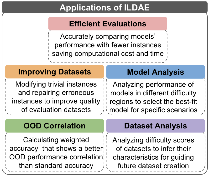
In this work, we address the above question by first computing difficulty scores of evaluation instances (section 2) and then demonstrating five novel applications of ILDAE (Figure 1).

1.

Efficient Evaluations: We propose an approach of conducting efficient-yet-accurate evaluations. Our approach uses as little as $5\%$ evaluation instances (selected via ILDAE) to achieve up to $0.93$ Kendall correlation with evaluations conducted using the complete dataset. Thus, without considerably impacting the outcome of evaluations, our approach saves computational cost and time.
2.

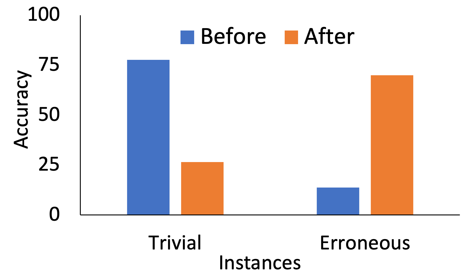
Improving Evaluation Datasets: We first show that ‘trivial’ and ‘erroneous’ instances can be identified using our difficulty scores and then present a model-and-human-in-the-loop technique to modify/repair such instances resulting in improved quality of the datasets. We instantiate it with SNLI dataset Bowman et al. (2015) and show that on modifying the trivial instances, the accuracy (averaged over $27$ models) drops from 77.58% to 26.49%, and on repairing the erroneous instances, it increases from 13.65% to 69.9%. Thus, improving the dataset quality.
3.

Model Analysis: We divide evaluation instances into different regions based on the difficulty scores and analyze models’ performance in each region. We find that a single model does not achieve the highest accuracy across all regions. This implies that different models are best suited for different types of questions and such analysis could benefit in model selection. For instance, in scenarios where a system is expected to encounter hard instances, the model that performs best in high difficulty regions should be preferred.
4.

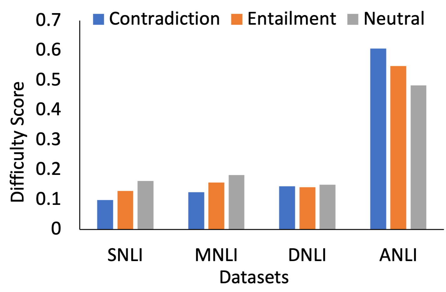
Dataset Analysis: ILDAE reveals several important characteristics of datasets that can be leveraged in future data creation processes. For instance, we find that in SNLI and MNLI datasets, ‘contradiction’ instances receive lower average difficulty score than ‘entailment’ and ‘neutral’ instances. Thus, more difficult contradiction examples can be created to develop high-quality task-specific datasets.
5.

OOD Correlation: We compute weighted accuracy leveraging the difficulty scores and show that it leads to $5.2\%$ higher Kendall correlation with Out-of-Domain (OOD) performance than the standard accuracy that treats all instances equally. Thus, ILDAE helps in getting a more reliable estimation of models’ OOD performance.

2 Difficulty Score Computation

2.1 Desiderata for Difficulty Scores

Interpretation:

Human perception of difficulty may not always correlate well with machine’s interpretation. Thus, difficulty scores must be computed via a model-in-the-loop technique so that they directly reflect machine’s interpretation.

Relationship with Predictive Correctness:

Difficulty scores must be negatively correlated with predictive correctness since a difficult instance is less likely to be predicted correctly than a relatively easier instance.

2.2 Method

Algorithm 1 Difficulty Score Computation

Input:

T

: Training Data,

M

: Model,

D

: Evaluation Data

E

: Training Epochs

Output: Difficulty Score of each instance in

D

Auxiliary Function: GET_CKPTS (

t_{r}

m

e

) - Returns checkpoints on training model

m

with data

t_{r}

for

e

epochs

Initialization:

Models\leftarrow\emptyset

: List to store ensemble of models trained with different configurations

\triangleright

Train with Partial Data

for each

pct\in[100,50,25,20,10,5]

T_{p}

= Sample(

T,pct

)

Models

+= Get_Ckpts(

T_{p}

M

E

)

end for each

\triangleright

Train with Corrupted Data

for each

pct\in[25,20,10,5,2]

T_{c}

= Corrupt(

T,pct

)

Models

+= Get_Ckpts(

T_{c}

M

E

)

end for each

\triangleright

Infer

D

using all

Models

and compute difficulty score

d_{i}

for each instance

i\in D

for each

i\in D

d_{i}=1-\dfrac{\sum_{m\in Models}c_{mi}}{|Models|}

\triangleright

where

c_{mi}

is the confidence assigned to the ground truth answer by model

m

end for each

return

d

We incorporate the above desiderata and consider model’s prediction confidence in the ground truth answer (indicated by softmax probability assigned to that answer) as the measure of its predictive correctness. Furthermore, we compile an ensemble of models trained with varying configurations and use their mean predictive correctness to compute the difficulty scores. We do this because model’s predictions fluctuate greatly when its training configuration is changed Zhou et al. (2020); McCoy et al. (2020) and relying on predictive correctness of only one model could result in difficulty scores that show poor generalization. To this end, we use the following three training configurations to compile predictions from an ensemble of models:

Data Size:

Instances that can be answered correctly even with few training examples are inherently easy and should receive lower difficulty score than the ones that require a large training dataset. To achieve this, we train a model each with 5, 10, 15, 20, 25, 50, and 100 % of the total training examples and include them in our ensemble.

Data Corruption:

Instances that can be answered correctly even with some level of corruption/noise in the training dataset should receive low difficulty score. To achieve this, we train a model each with different levels of noise (2, 5, 10, 20, 25% of the examples) in the training data, and add them to our ensemble. For creating noisy examples, we randomly change the ground-truth label in case of classification and multiple-choice datasets and change the answer span for extractive QA datasets.

Training Steps:

Instances that can be consistently answered correctly from the early stages of training should receive low difficulty score. Here, we add a model checkpoint after every epoch during training to our ensemble.

This results in a total of $N=E*(7+5)$ models in our ensemble where $E$ corresponds to the number of training epochs, and $7$ , $5$ correspond to the number of data size and data corruption configurations respectively. We infer the evaluation dataset using these $N$ models and calculate the average predictive correctness for each instance. Finally, we compute the difficulty score by subtracting this averaged correctness value from $1$ . This ensures that an instance that is answered correctly with high confidence under many training configurations gets assigned a low difficulty score as it corresponds to an easy instance. In contrast, an instance that is often answered incorrectly gets assigned a high difficulty score. Algorithm 1 summarizes this approach.

We use RoBERTa-large model Liu et al. (2019) for this procedure and train each model for $E=10$ epochs, resulting in $N=120$ predictions for each evaluation instance. Our difficulty computation method is general and can be used with any other model or configurations; we use RoBERTa-large as it has been shown to achieve high performance across diverse NLP tasks Liu et al. (2019). In addition, we show that difficulty scores computed using our procedure also generalize for other models (3.5.1).

We note that difficulty computation is not our primary contribution. Prior work Swayamdipta et al. (2020); Xu et al. (2020) has explored different ways to achieve this. However, our approach uses $120$ predictions from models trained with different configurations for its computation and hence is more reliable. Equipped with difficulty scores of evaluation instances, we now demonstrate five applications of ILDAE in the following sections.

3 Efficient Evaluations

3.1 Problem Statement

Success of BERT Devlin et al. (2019) has fostered development of several other pre-trained language models such as RoBERTa Liu et al. (2019), XLNet Yang et al. (2019b), DistilBERT Sanh et al. (2019), ALBERT Lan et al. (2020). Though, it has resulted in the availability of numerous model options for a task, comparing the performance of such a large number of models has become computationally expensive and time-consuming. For example, in real-world applications like online competitions, the naive approach that evaluates candidate models on the entire test dataset would be too expensive because they receive thousands of model submissions and contain a sizable number of evaluation instances. Moreover, some applications also require additional evaluations to measure Out-of-Domain generalization and robustness making it even more expensive. Can we make the evaluations efficient?

3.2 Solution

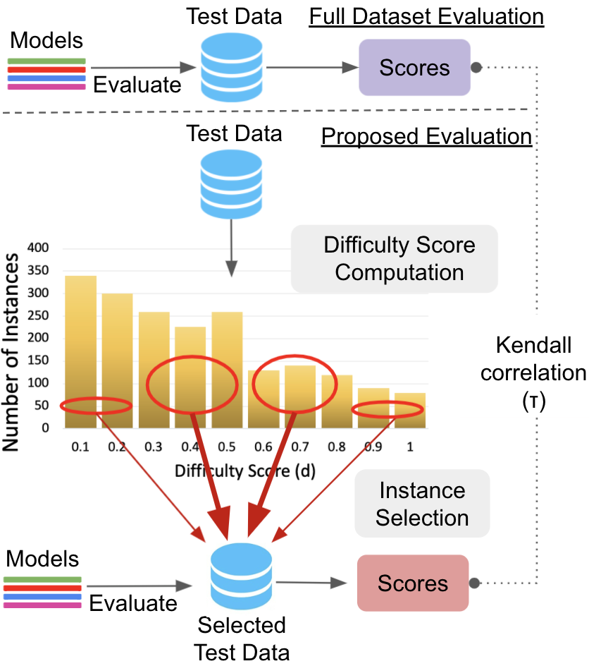
We address the above question and explore if the performance of candidate models can be accurately compared with a carefully selected smaller subset of the evaluation dataset. Reducing the number of instances would save computational cost and make the evaluations efficient. To this end, we propose an approach that selects evaluation instances based on their difficulty scores. We compare performance of candidate models only on these selected instances and show that without considerably impacting the result of evaluations, our approach saves computational cost and time.

Instance Selection: We argue that the instances with extreme difficulty scores (very low and very high scores) would not be very effective in distinguishing between the candidate models. This is because the former instances are trivial and would be answered correctly by many/all candidate models, while the latter ones are hard and would be answered correctly by only a few/none models. Therefore, given a budget on the number of evaluation instances, we select a majority of them with moderate difficulty scores. However, to distinguish amongst very weak and amongst very strong candidates, we also include a small number of instances with extreme difficulty scores. Figure 2 illustrates our approach.

Note that our approach does not add any computational overhead during evaluations as the difficulty scores are pre-computed. Furthermore, we do not compute separate difficulty scores for each candidate model as it would defy the sole purpose of ‘efficient’ evaluations. Instead, we compute difficulty scores using only one model (RoBERTa-large) and exclude it from the list of candidate models for a fair evaluation of our approach. For our instance selection approach to work in this setting, the difficulty scores should generalize for other models. We empirically prove this generalization capability and demonstrate the efficacy of our efficient evaluations approach in 3.5.

3.3 Experimental Details

Performance Metric:

We measure the efficacy of an instance selection technique by computing accuracies of candidate models on the selected instances and calculating their Kendall’s correlation Kendall (1938) with accuracies obtained on the full evaluation dataset. High correlation implies that the performance scores obtained using the selected instances display the same behavior as the performance scores obtained using the complete dataset. Hence, high correlations values are preferred.

Datasets:

We experiment with a total of $23$ datasets across Natural Language Inference, Duplicate Detection, Sentiment Analysis, Question Answering, Commonsense Reasoning, and several other tasks. Refer to Appendix section B for an exhaustive list of datasets for each task.

Candidate Models:

We use BERT Devlin et al. (2019), DistilBERT Sanh et al. (2019), ConvBERT Jiang et al. (2020) , XLNET Yang et al. (2019a), SqueezeBERT Iandola et al. (2020), ELECTRA Clark et al. (2020) in our experiments. We also use different variants of ConvBert (small, medium-small, base) and ELECTRA (small, base) models. For comprehensive experiments, we train each of the above models with training data of three different sizes ( $2k$ , $5k$ , and $10k$ examples) resulting in $27$ candidate models for each dataset. We intentionally exclude RoBERTa from this list as we use it for computing the difficulty scores.

% Instances $\rightarrow$	0.5%			1%			2%	5%	10%	20%
Dataset $\downarrow$	Random	Heuristic	Proposed	Random	Heuristic	Proposed	Proposed	Proposed	Proposed	Proposed
SNLI	$0.55_{0.09}$	$0.38_{0.17}$	$\textbf{0.68}_{0.13}$	$0.68_{0.05}$	$0.58_{0.08}$	$\textbf{0.78}_{0.08}$	$0.83_{0.04}$	$0.88_{0.04}$	$0.91_{0.01}$	$0.93_{0.02}$
PAWS Wiki	$0.67_{0.07}$	$0.68_{0.04}$	$\textbf{0.78}_{0.06}$	$0.73_{0.05}$	$0.78_{0.02}$	$\textbf{0.86}_{0.05}$	$0.89_{0.02}$	$0.91_{0.03}$	$0.95_{0.01}$	$0.96_{0.01}$
AgNews	$0.12_{0.26}$	$0.14_{0.27}$	$\textbf{0.47}_{0.05}$	$0.25_{0.34}$	$0.41_{0.14}$	$\textbf{0.52}_{0.1}$	$0.65_{0.07}$	$0.75_{0.06}$	$0.8_{0.04}$	$0.89_{0.03}$
QNLI	$0.41_{0.1}$	$0.44_{0.04}$	$\textbf{0.48}_{0.13}$	$0.57_{0.04}$	$0.55_{0.1}$	$\textbf{0.57}_{0.07}$	$0.7_{0.06}$	$0.78_{0.06}$	$0.85_{0.03}$	$0.91_{0.03}$
MRPC	$0.04_{0.09}$	$-0.03_{0.18}$	$\textbf{0.21}_{0.16}$	$-0.02_{0.09}$	$0.05_{0.2}$	$\textbf{0.29}_{0.21}$	$0.36_{0.15}$	$0.45_{0.08}$	$0.58_{0.12}$	$0.65_{0.14}$
SocialIQA	$0.19_{0.09}$	$0.15_{0.29}$	$\textbf{0.37}_{0.17}$	$0.34_{0.07}$	$0.28_{0.21}$	$\textbf{0.4}_{0.09}$	$0.58_{0.1}$	$0.67_{0.04}$	$0.75_{0.08}$	$0.81_{0.05}$
QQP	$0.63_{0.06}$	$0.64_{0.05}$	$\textbf{0.65}_{0.05}$	$0.74_{0.03}$	$0.74_{0.01}$	$\textbf{0.77}_{0.06}$	$0.84_{0.04}$	$0.9_{0.04}$	$0.94_{0.04}$	$0.95_{0.01}$
DNLI	$0.58_{0.05}$	$0.59_{0.1}$	$\textbf{0.58}_{0.11}$	$0.68_{0.1}$	$0.71_{0.04}$	$\textbf{0.76}_{0.07}$	$0.84_{0.04}$	$0.92_{0.05}$	$0.94_{0.03}$	$0.96_{0.01}$
COLA	$-$	$-$	$-$	$-0.01_{0.18}$	$\textbf{0.25}_{0.26}$	$0.24_{0.45}$	$0.41_{0.41}$	$0.63_{0.23}$	$0.75_{0.08}$	$0.78_{0.02}$
SWAG	$0.72_{0.04}$	$0.66_{0.02}$	$\textbf{0.75}_{0.06}$	$0.79_{0.03}$	$0.77_{0.03}$	$\textbf{0.78}_{0.05}$	$0.86_{0.03}$	$0.89_{0.02}$	$0.93_{0.01}$	$0.95_{0.01}$
PAWS QQP	$-$	$-$	$-$	$0.13_{0.24}$	$0.36_{0.05}$	$\textbf{0.34}_{0.13}$	$0.55_{0.19}$	$0.8_{0.05}$	$0.84_{0.03}$	$0.87_{0.04}$
MNLI	$0.7_{0.04}$	$0.71_{0.03}$	$\textbf{0.73}_{0.07}$	$0.8_{0.02}$	$0.8_{0.04}$	$\textbf{0.82}_{0.08}$	$0.89_{0.03}$	$0.93_{0.02}$	$0.95_{0.02}$	$0.96_{0.01}$
Adv. NLI R1	$0.0_{0.08}$	$-0.07_{0.06}$	$\textbf{0.17}_{0.27}$	$0.02_{0.13}$	$\textbf{0.09}_{0.11}$	$0.08_{0.2}$	$0.13_{0.18}$	$0.3_{0.18}$	$0.47_{0.05}$	$0.59_{0.05}$
Adv. NLI R2	$-0.08_{0.04}$	$\textbf{-0.01}_{0.06}$	$-0.08_{0.16}$	$-0.08_{0.07}$	$\textbf{0.02}_{0.03}$	$-0.03_{0.21}$	$0.0_{0.12}$	$0.17_{0.03}$	$0.26_{0.11}$	$0.42_{0.15}$
Adv. NLI R3	$-0.15_{0.12}$	$\textbf{0.15}_{0.1}$	$0.1_{0.21}$	$-0.03_{0.06}$	$0.07_{0.1}$	$\textbf{0.1}_{0.11}$	$0.18_{0.16}$	$0.12_{0.17}$	$0.31_{0.15}$	$0.58_{0.05}$
SST-2	$-$	$-$	$-$	$0.08_{0.15}$	$0.16_{0.35}$	$\textbf{0.29}_{0.25}$	$0.4_{0.2}$	$0.52_{0.16}$	$0.65_{0.13}$	$0.81_{0.08}$
ARC Easy	$-$	$-$	$-$	$0.0_{0.2}$	$-0.03_{0.12}$	$\textbf{0.42}_{0.19}$	$0.47_{0.19}$	$0.59_{0.13}$	$0.6_{0.14}$	$0.74_{0.11}$
ARC Diff	$-$	$-$	$-$	$-$	$-$	$-$	$0.15_{0.29}$	$0.28_{0.13}$	$0.33_{0.31}$	$0.3_{0.26}$
Abductive NLI	$0.08_{0.26}$	$\textbf{0.17}_{0.05}$	$0.16_{0.09}$	$0.19_{0.19}$	$0.26_{0.08}$	$\textbf{0.3}_{0.07}$	$0.42_{0.13}$	$0.57_{0.08}$	$0.61_{0.07}$	$0.68_{0.07}$
Winogrande	$-0.19_{0.11}$	$-0.03_{0.06}$	$\textbf{0.0}_{0.17}$	$-0.11_{0.09}$	$-0.05_{0.12}$	$\textbf{0.11}_{0.15}$	$0.09_{0.14}$	$0.03_{0.1}$	$0.14_{0.1}$	$0.21_{0.14}$
CSQA	$0.29_{0.11}$	$0.28_{0.1}$	$\textbf{0.31}_{0.07}$	$0.36_{0.14}$	$0.37_{0.08}$	$\textbf{0.39}_{0.09}$	$0.49_{0.09}$	$0.69_{0.08}$	$0.78_{0.04}$	$0.83_{0.05}$
QuaRel	$-$	$-$	$-$	$-$	$-$	$-$	$0.32_{0.26}$	$0.33_{0.25}$	$0.39_{0.07}$	$0.51_{0.1}$
QuaRTz	$-$	$-$	$-$	$-$	$-$	$-$	$0.34_{0.19}$	$0.36_{0.04}$	$0.34_{0.12}$	$0.37_{0.08}$
Average	$0.28_{0.1}$	$0.3_{0.11}$	$\textbf{0.39}_{0.13}$	$0.31_{0.11}$	$0.35_{0.11}$	$\textbf{0.43}_{0.14}$	$0.46_{0.17}$	$0.58_{0.11}$	$0.66_{0.08}$	$0.72_{0.07}$

Table 1: Kendall correlation with full evaluation dataset achieved by various instance selection approaches for different percentage of instances. Each cell shows the mean and standard deviation obtained from 5 different runs.

-

cell indicates 0 selected instances. We show the expanded version of this table in supplementary.

Instance Selection Baselines:

We compare the proposed instance selection approach with the following baselines:

Random Selection: Select a random subset of instances from the evaluation dataset.

Heuristic Selection: Select instances based on the length heuristic (number of characters in the instance text) instead of the difficulty scores.

3.4 Related Work

Adaptive evaluation Weiss (1982) is used in educational settings for evaluating performance of students. It uses Item Response Theory (IRT) Baker and Kim (2004) from psychometrics which requires a large number of subjects and items to estimate system parameters Lalor et al. (2016, 2018). Moreover, adaptive evaluation is computationally very expensive as it requires calculating the performance after each response and then selecting the next instance based on the previous responses of the subject. Thus, it is not fit for our setting as we intend to improve the computational efficiency. In contrast, our approach is much simpler and efficient as it does not incur any additional cost during evaluation.

3.5 Results

We first study generalization of our computed difficulty scores and then show the efficacy of the proposed instance selection approach in conducting efficient evaluations.

3.5.1 Generalization of Difficulty Scores:

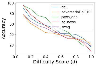
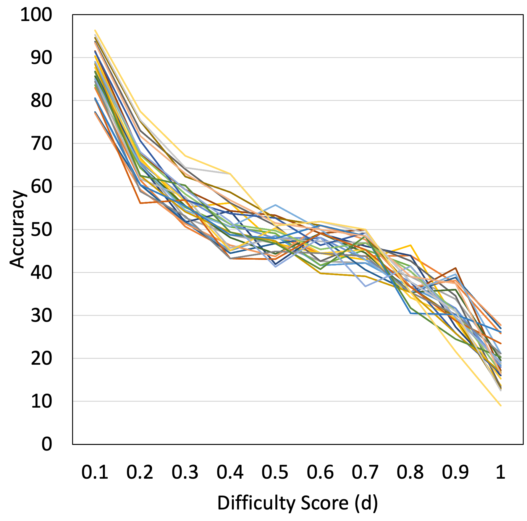
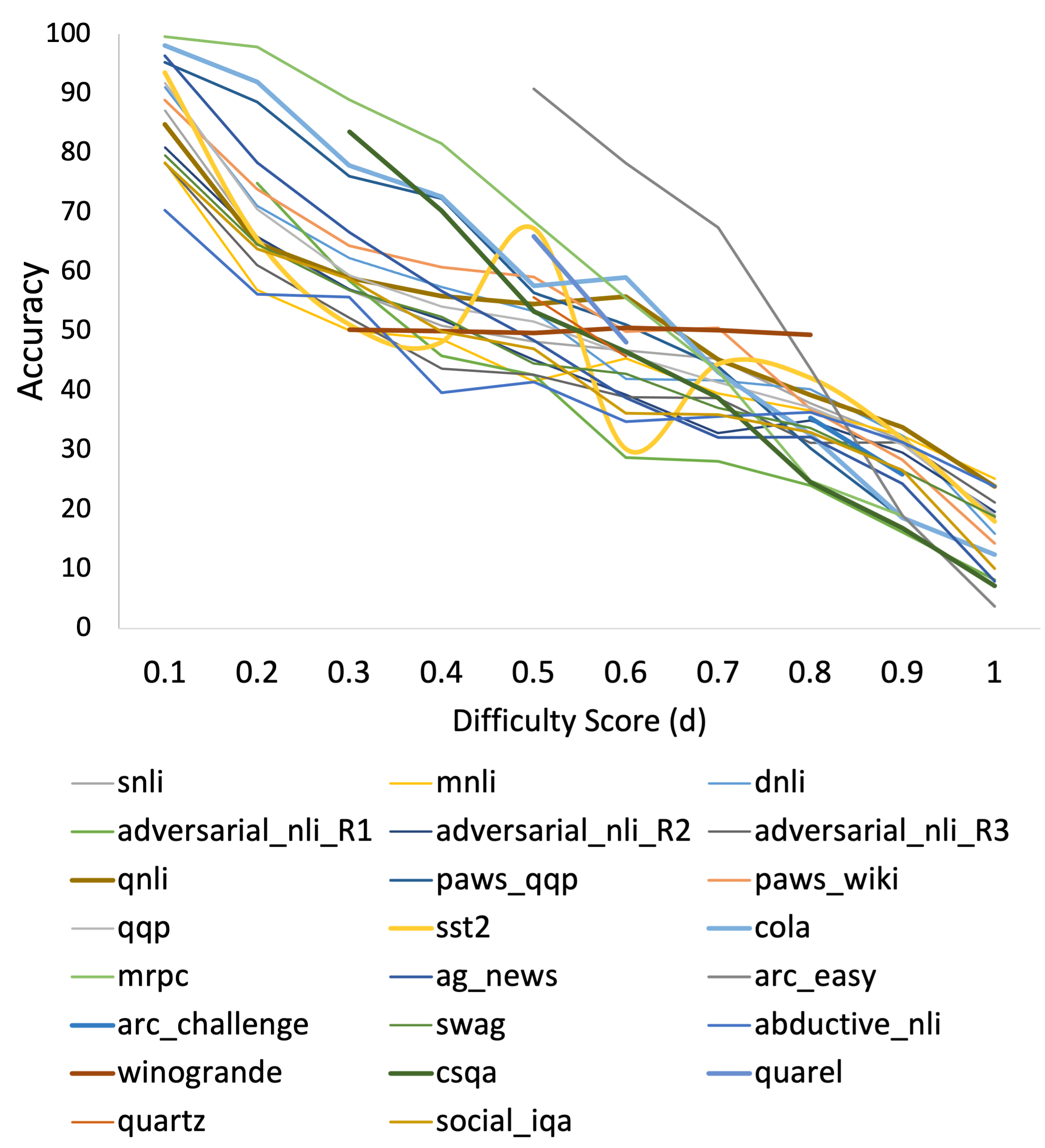
In Figure 3, we plot accuracy (averaged over all 27 candidate models) against difficulty scores (computed using RoBERTa-large). We find that with the increase in difficulty score, the accuracy consistently decreases for all datasets. We also study this behavior for each individual candidate model and find results supporting the above observation²²2Further details are in appendix (Figure 6). This proves that the difficulty scores follow the desiderata mentioned in Section 2.1 for other models also and our intuitions behind instance selection for conducting efficient evaluations hold true. Note that these difficulty scores are computed using a specific model but our approach is general and will replicate this generalization capability if used with any other model.

3.5.2 Efficient Evaluations:

Table 1 shows Kendall correlation with full dataset evaluation achieved by various instance selection approaches for different percentages of instances.

Proposed Approach Outperforms Baselines:

Our proposed approach is consistently better than the Random and Heuristic approaches. For instance, with just $0.5\%$ and $1\%$ evaluation instances, our approach outperforms the baseline methods by $\sim 30\%$ and $\sim 22.8\%$ respectively. We show the expanded version of this table and performance of other instance selection techniques in Appendix.

Correlation Change with % of Instances:

As expected, Kendall correlation consistently increases as a higher percentage of instances are selected for evaluation. In case of SNLI, PAWS Wiki, QQP, DNLI, SWAG, and MNLI, just $2\%$ instances are sufficient to achieve correlation of $>0.8$ . For most datasets, with just $20\%$ of the evaluation instances, our approach achieves Kendall correlation of $>0.8$ . This suggests that the evaluations can be conducted with fewer instances without significantly compromising the accuracy of comparison. We further analyze performance of our approach for higher percentage of instances in Table 4.

Thus, for practical settings where candidate models can’t be compared on the entire dataset due to computational and time constraints, evaluating only on the selected instances can result in fairly accurate performance comparison.

Performance on Multiple-Choice QA datasets:

Though, we perform better than the baselines approaches on almost all datasets, we achieve a lower correlation value for multiple-choice question answering datasets such as QuaRel, QuaRTz, and Winogrande. We attribute this behavior to the close scores (accuracies) achieved by many candidate models even in case of full dataset evaluation. Thus, it is difficult to differentiate such models as they achieve nearly the same performance. Furthermore, in some difficult datasets such as Adversarial NLI (R1, R2, and R3), ARC Difficult, and Winogrande, many candidate models achieve accuracies very close to the random baseline ( $33\%$ for NLI, $50\%$ for Winogrande). So, comparing their performance even with full dataset does not provide any significant insights.

4 Improving Evaluation Datasets

4.1 Problem Statement

Recent years have seen a rapid increase in the number and size of NLP datasets. Crowd-sourcing is a prominent way of collecting these datasets. Prior work Gururangan et al. (2018); Tan et al. (2019); Mishra et al. (2020) has shown that crowd-sourced datasets can contain: (a) erroneous instances that have annotation mistakes or ambiguity, (b) too many trivial instances that are very easy to answer. This hampers the quality of the dataset and makes it less reliable for drawing conclusions. Can difficulty scores aid in improving the quality of evaluation datasets?

Dataset	Instance
SNLI (72%)	Premise: Trucks racing. Hypothesis: Four trucks are racing against each other in the relay. Label: Entailment, Neutral
CSQA (50%)	Why would a band be performing when there are no people nearby? O1: record album, O2: play music, O3: hold concert, O4: blaring, O5: practice
WG (36%)	Maria was able to keep their weight off long term, unlike Felicia, because _ followed a healthy diet. O1: Maria, O2: Felicia
aNLI (x%)	O1: Ella was taking her final exam. O2: Ella was able to finish her exam on time. H1: Ella got to class early and was in no hurry. H2: Ella broke her pencil.

Table 2: Examples of erroneous instances from SNLI, CSQA, Winogrande, and Abductive NLI. Orange (ambiguous) and red (mislabeled) correspond to the originally annotated answer while blue corresponds to the correct/equally probable answer.

4.2 Solution

We first show that erroneous and trivial instances can be identified using the difficulty scores and then present a human-and-model-in-the-loop technique to modify/repair such instances resulting in improved quality of the datasets.

Identifying Erroneous and Trivial Instances:

We inspect $50$ instances each with very high and very low difficulty scores and find that a significant percentage of the former are either mislabeled or contain ambiguity and the latter are too easy to be answered.

Table 2 shows examples of erroneous instances from SNLI, Winogrande, CSQA, and Abductive NLI. We find $72\%$ of the inspected SNLI instances to be erroneous. Furthermore, we find that some high difficulty score instances are actually difficult even for humans because they require abilities such as commonsense reasoning. Table 5 (appendix) shows such instances. We also provide examples of trivial instances (Table 7) and note that such instances are trivial from model’s perspective as they can be answered correctly (with high confidence) by simply latching on to some statistical cues present in the training data.

Technique:

Since the trivial instances are too easy to be answered, we propose to modify them in an adversarial way such that they no longer remain trivial. Specifically, we include a human-in-the-loop who needs to modify a trivial instance in a label-preserving manner such that the modified version fools the model into making an incorrect prediction. For adversarial attack, we use the strongest model from our ensemble of $120$ models. It has two key differences with the standard adversarial data creation approach presented in Nie et al. (2020); Kiela et al. (2021): (a) it requires modifying an already existing instance instead of creating a new instance from scratch. (b) it does not increase the size of the evaluation dataset as we replace an already saturated instance (trivial) with its improved not-trivial version. We use a human instead of leveraging automated ways to modify the trivial instances because our objective is to improve the quality of instances and prior work has shown that these automated techniques often result in unnatural and noisy instances. Therefore, such techniques could be cost-efficient but might not solve the sole purpose of improving quality.

To further improve the quality, we provide instances with very high difficulty score (potentially erroneous) and ask a human to repair them such that the repaired versions follow the task definition. The human can either change the instance text or its answer to achieve the goal. Note that this scenario is model-independent.

4.3 Results

Table 3 shows original and modified instances from SNLI. Top two examples correspond to the trivial instances where the human modified the hypothesis in a label-preserving manner such that it fooled the model into making incorrect prediction. The bottom two correspond to the mislabeled instances where the human rectified the label. Figure 4 compares the performance of models on the original instances and the their modified/repaired versions. As expected, the performance drops on the previously trivial instances as they are no longer trivial and improves on the previously erroneous instances. We release the improved version of the dataset compiled via our technique.

Original Instance	Modification
P: A man standing in front of a chalkboard points at a drawing. H: A kid washes a chalkboard L: Contradiction	H’: A 4 year old male standing in front of a chalkboard points at a drawing. Predicted L: Neutral
P: A man is performing tricks with his superbike. H: A bike is in the garage. L: Contradiction	H’: He is performing stunts on a four wheeler. Predicted L: Neutral
P: A skateboarder does a trick at a skate park. H: The skateboarder is performing a heelie kick flip. L: Entailment	L’: Neutral
P: A little blond girl is running near a little blond boy. H: A sister and brother are playing in their yard. L: Entailment	L’: Neutral

Table 3: Illustrative examples from SNLI dataset modified using our technique. Top two correspond to trivial instances for which a human modified the hypothesis in a label-preserving manner such that the model’s prediction changed. Bottom two correspond to mislabeled instances where the human rectified the label.

5 Other Applications of ILDAE

We now briefly discuss other ILDAE applications.

5.1 Dataset Analysis

ILDAE reveals several useful characteristics of datasets such as which class label has the easiest instances. We study this for NLI datasets: SNLI, MNLI, DNLI, and Adversarial NLI (Figure 5). For SNLI and MNLI, we find that the contradiction instances receive lower average difficulty score than entailment and neutral instances. For Adversarial NLI, the order is reversed. For DNLI, all the labels get assigned nearly the same average difficulty. Such analysis can serve as a guide for future data creation as it indicates for which type of instances more data collection effort needs to be invested. It can also be used to compare average difficulty at dataset level. Furthermore, a new harder task-specific benchmark can be created by combining high difficulty instances from all the datasets of that task.

5.2 Model Analysis

We divide the evaluation instances into different regions based on the difficulty scores and analyze models’ performance in each region. We find that a single model does not achieve the highest accuracy across all regions. Figure 6 illustrates this pattern for SNLI dataset. This implies that the model that achieves the highest performance on easy instances may not necessarily achieve the highest performance on difficult instances. The similar pattern is observed for other datasets (refer appendix). Such analysis would benefit in model selection. For instance, in scenarios where a system is expected to encounter hard instances, we can select the model that has the highest accuracy on instances of difficult regions. Whereas, for scenarios containing easy instances, the model that has the highest accuracy on instances of easy regions.

5.3 Correlation with OOD Performance

Large pre-trained language models can achieve high In-Domain performance on numerous tasks. However, it does not correlate well with OOD performance Hendrycks and Dietterich (2019); Hendrycks et al. (2020). To this end, we present an approach to compute a weighted accuracy that shifts away from treating all the evaluations instances equally and assigns weight based on their difficulty scores. We define the weight $w_{i}$ of an instance $i$ with difficulty score $d_{i}$ as:

w_{i}=\frac{1+\mu*d_{i}}{N+\mu*\sum_{j=1}^{N}d_{j}}

where $N$ corresponds to the total number of evaluation instances, and $\mu$ is a hyper-parameter that controls influence of difficulty score on the weight. Then, weighted accuracy $W$ is simply:

W=\sum_{i=1}^{N}w_{i}*v_{i}

where $v_{i}$ is 1 when the model’s prediction is correct else 0. This implies that high accuracy may not always translate to high weighted accuracy.

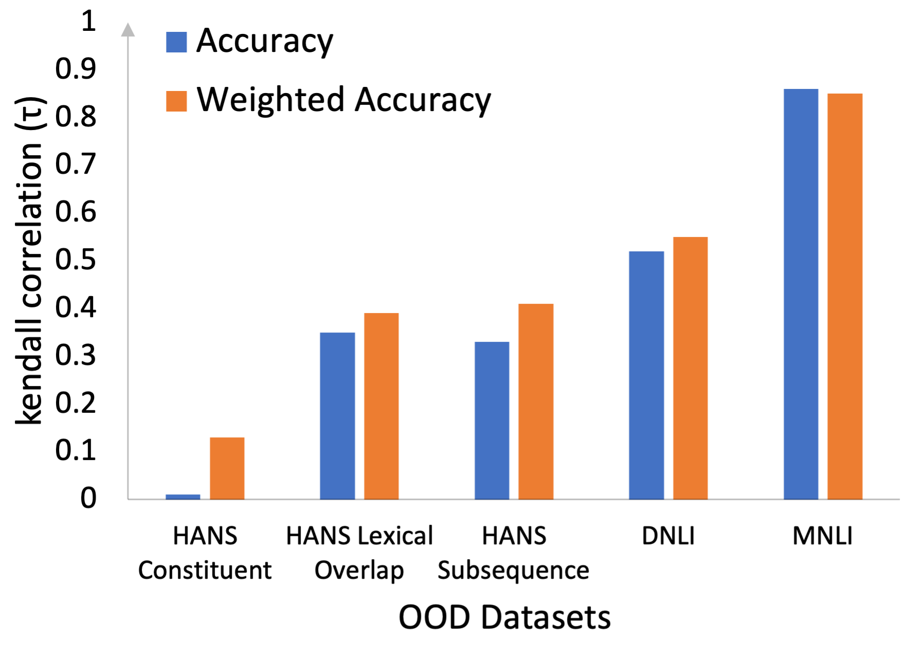
We take SNLI as the in-domain dataset and MNLI, DNLI, and HANS McCoy et al. (2019) (Constituent, Lexical Overlap, Subsequence) as OOD datasets. We calculate unweighted and weighted accuracy of the 27 models (described in Section 3.3) and compare their Kendall correlation with the accuracy on OOD datasets. Figure 7 shows this comparison. It can be observed that weighted accuracy shows $5.2\%$ higher correlation with OOD performance. Most improvement is observed in datasets that have many instances with high difficulty score (HANS). Thus, weighting instances based on their difficulty score is more informative than the standard accuracy.

6 Conclusion

We conducted Instance-Level Difficulty Analysis of Evaluation data (ILDAE) in a large-scale setup of $23$ datasets and presented its five novel applications. With these applications, we demonstrated ILDAE’s impact in several important areas, such as conducting efficient evaluations with fewer instances, improving dataset quality, and estimating out-of-domain performance reliably. We release our computed difficulty scores and hope that our analyses and findings will bring more attention to this important yet underexplored field of leveraging instance difficulty in evaluations.

Ethical Considerations

We use existing public-domain text datasets, such as SNLI, Winogrande, and ARC, and follow the protocol to use and adapt research data to compute instance-level difficulty scores. We will release the computed difficulty scores, but will not share the original source data. We recommend readers to refer to the original source research papers. Any bias observed in difficulty scores computed using our methods can be attributed to the source data and our computation functions. However, no particular socio-political bias is emphasized or reduced specifically by our methods.

References

Baker and Kim (2004) Frank B Baker and Seock-Ho Kim. 2004. Item response theory: Parameter estimation techniques. CRC Press.
Bhagavatula et al. (2020) Chandra Bhagavatula, Ronan Le Bras, Chaitanya Malaviya, Keisuke Sakaguchi, Ari Holtzman, Hannah Rashkin, Doug Downey, Wen tau Yih, and Yejin Choi. 2020. Abductive commonsense reasoning. In International Conference on Learning Representations.
Bowman et al. (2015) Samuel R. Bowman, Gabor Angeli, Christopher Potts, and Christopher D. Manning. 2015. A large annotated corpus for learning natural language inference. In Proceedings of the 2015 Conference on Empirical Methods in Natural Language Processing, pages 632–642, Lisbon, Portugal. Association for Computational Linguistics.
Clark et al. (2020) Kevin Clark, Minh-Thang Luong, Quoc V. Le, and Christopher D. Manning. 2020. ELECTRA: Pre-training text encoders as discriminators rather than generators. In ICLR.
Clark et al. (2018) Peter Clark, Isaac Cowhey, Oren Etzioni, Tushar Khot, Ashish Sabharwal, Carissa Schoenick, and Oyvind Tafjord. 2018. Think you have solved question answering? try arc, the ai2 reasoning challenge. arXiv preprint arXiv:1803.05457.
Devlin et al. (2019) Jacob Devlin, Ming-Wei Chang, Kenton Lee, and Kristina Toutanova. 2019. BERT: Pre-training of deep bidirectional transformers for language understanding. In Proceedings of the 2019 Conference of the North American Chapter of the Association for Computational Linguistics: Human Language Technologies, Volume 1 (Long and Short Papers), pages 4171–4186, Minneapolis, Minnesota. Association for Computational Linguistics.
Dolan and Brockett (2005) William B Dolan and Chris Brockett. 2005. Automatically constructing a corpus of sentential paraphrases. In Proceedings of the Third International Workshop on Paraphrasing (IWP2005).
Gururangan et al. (2018) Suchin Gururangan, Swabha Swayamdipta, Omer Levy, Roy Schwartz, Samuel Bowman, and Noah A. Smith. 2018. Annotation artifacts in natural language inference data. In Proceedings of the 2018 Conference of the North American Chapter of the Association for Computational Linguistics: Human Language Technologies, Volume 2 (Short Papers), pages 107–112, New Orleans, Louisiana. Association for Computational Linguistics.
Hendrycks and Dietterich (2019) Dan Hendrycks and Thomas Dietterich. 2019. Benchmarking neural network robustness to common corruptions and perturbations. In International Conference on Learning Representations.
Hendrycks et al. (2020) Dan Hendrycks, Xiaoyuan Liu, Eric Wallace, Adam Dziedzic, Rishabh Krishnan, and Dawn Song. 2020. Pretrained transformers improve out-of-distribution robustness. In Proceedings of the 58th Annual Meeting of the Association for Computational Linguistics, pages 2744–2751, Online. Association for Computational Linguistics.
Iandola et al. (2020) Forrest Iandola, Albert Shaw, Ravi Krishna, and Kurt Keutzer. 2020. SqueezeBERT: What can computer vision teach NLP about efficient neural networks? In Proceedings of SustaiNLP: Workshop on Simple and Efficient Natural Language Processing, pages 124–135, Online. Association for Computational Linguistics.
Iyer et al. (2017) Shankar Iyer, Nikhil Dandekar, and Kornél Csernai. 2017. First quora dataset release: Question pairs. data. quora. com.
Jiang et al. (2020) Zi-Hang Jiang, Weihao Yu, Daquan Zhou, Yunpeng Chen, Jiashi Feng, and Shuicheng Yan. 2020. Convbert: Improving bert with span-based dynamic convolution. In Advances in Neural Information Processing Systems, volume 33, pages 12837–12848. Curran Associates, Inc.
Kendall (1938) Maurice G Kendall. 1938. A new measure of rank correlation. Biometrika, 30(1/2):81–93.
Kiela et al. (2021) Douwe Kiela, Max Bartolo, Yixin Nie, Divyansh Kaushik, Atticus Geiger, Zhengxuan Wu, Bertie Vidgen, Grusha Prasad, Amanpreet Singh, Pratik Ringshia, Zhiyi Ma, Tristan Thrush, Sebastian Riedel, Zeerak Waseem, Pontus Stenetorp, Robin Jia, Mohit Bansal, Christopher Potts, and Adina Williams. 2021. Dynabench: Rethinking benchmarking in NLP. In Proceedings of the 2021 Conference of the North American Chapter of the Association for Computational Linguistics: Human Language Technologies, pages 4110–4124, Online. Association for Computational Linguistics.
Lalor et al. (2018) John P. Lalor, Hao Wu, Tsendsuren Munkhdalai, and Hong Yu. 2018. Understanding deep learning performance through an examination of test set difficulty: A psychometric case study. In Proceedings of the 2018 Conference on Empirical Methods in Natural Language Processing, pages 4711–4716, Brussels, Belgium. Association for Computational Linguistics.
Lalor et al. (2016) John P. Lalor, Hao Wu, and Hong Yu. 2016. Building an evaluation scale using item response theory. In Proceedings of the 2016 Conference on Empirical Methods in Natural Language Processing, pages 648–657, Austin, Texas. Association for Computational Linguistics.
Lan et al. (2020) Zhenzhong Lan, Mingda Chen, Sebastian Goodman, Kevin Gimpel, Piyush Sharma, and Radu Soricut. 2020. Albert: A lite bert for self-supervised learning of language representations. In International Conference on Learning Representations.
Liu et al. (2019) Yinhan Liu, Myle Ott, Naman Goyal, Jingfei Du, Mandar Joshi, Danqi Chen, Omer Levy, M. Lewis, Luke Zettlemoyer, and Veselin Stoyanov. 2019. Roberta: A robustly optimized bert pretraining approach. ArXiv, abs/1907.11692.
McCoy et al. (2020) R. Thomas McCoy, Junghyun Min, and Tal Linzen. 2020. BERTs of a feather do not generalize together: Large variability in generalization across models with similar test set performance. In Proceedings of the Third BlackboxNLP Workshop on Analyzing and Interpreting Neural Networks for NLP, pages 217–227, Online. Association for Computational Linguistics.
McCoy et al. (2019) Tom McCoy, Ellie Pavlick, and Tal Linzen. 2019. Right for the wrong reasons: Diagnosing syntactic heuristics in natural language inference. In Proceedings of the 57th Annual Meeting of the Association for Computational Linguistics, pages 3428–3448, Florence, Italy. Association for Computational Linguistics.
Mishra and Arunkumar (2021) Swaroop Mishra and Anjana Arunkumar. 2021. How robust are model rankings: A leaderboard customization approach for equitable evaluation. In Proceedings of the AAAI Conference on Artificial Intelligence, volume 35, pages 13561–13569.
Mishra et al. (2020) Swaroop Mishra, Anjana Arunkumar, Bhavdeep Sachdeva, Chris Bryan, and Chitta Baral. 2020. Dqi: Measuring data quality in nlp. arXiv preprint arXiv:2005.00816.
Mishra and Sachdeva (2020) Swaroop Mishra and Bhavdeep Singh Sachdeva. 2020. Do we need to create big datasets to learn a task? In Proceedings of SustaiNLP: Workshop on Simple and Efficient Natural Language Processing, pages 169–173, Online. Association for Computational Linguistics.
Nie et al. (2020) Yixin Nie, Adina Williams, Emily Dinan, Mohit Bansal, Jason Weston, and Douwe Kiela. 2020. Adversarial NLI: A new benchmark for natural language understanding. In Proceedings of the 58th Annual Meeting of the Association for Computational Linguistics, pages 4885–4901, Online. Association for Computational Linguistics.
Rodriguez et al. (2021) Pedro Rodriguez, Joe Barrow, Alexander Miserlis Hoyle, John P. Lalor, Robin Jia, and Jordan Boyd-Graber. 2021. Evaluation examples are not equally informative: How should that change NLP leaderboards? In Proceedings of the 59th Annual Meeting of the Association for Computational Linguistics and the 11th International Joint Conference on Natural Language Processing (Volume 1: Long Papers), pages 4486–4503, Online. Association for Computational Linguistics.
Sagawa et al. (2020) Shiori Sagawa, Aditi Raghunathan, Pang Wei Koh, and Percy Liang. 2020. An investigation of why overparameterization exacerbates spurious correlations. In International Conference on Machine Learning, pages 8346–8356. PMLR.
Sakaguchi et al. (2020) Keisuke Sakaguchi, Ronan Le Bras, Chandra Bhagavatula, and Yejin Choi. 2020. Winogrande: An adversarial winograd schema challenge at scale. In AAAI.
Sanh et al. (2019) Victor Sanh, Lysandre Debut, Julien Chaumond, and Thomas Wolf. 2019. Distilbert, a distilled version of bert: smaller, faster, cheaper and lighter. ArXiv, abs/1910.01108.
Sap et al. (2019) Maarten Sap, Hannah Rashkin, Derek Chen, Ronan Le Bras, and Yejin Choi. 2019. Social iqa: Commonsense reasoning about social interactions. In EMNLP 2019.
Socher et al. (2013) Richard Socher, Alex Perelygin, Jean Wu, Jason Chuang, Christopher D. Manning, Andrew Ng, and Christopher Potts. 2013. Recursive deep models for semantic compositionality over a sentiment treebank. In Proceedings of the 2013 Conference on Empirical Methods in Natural Language Processing, pages 1631–1642, Seattle, Washington, USA. Association for Computational Linguistics.
Swayamdipta et al. (2020) Swabha Swayamdipta, Roy Schwartz, Nicholas Lourie, Yizhong Wang, Hannaneh Hajishirzi, Noah A. Smith, and Yejin Choi. 2020. Dataset cartography: Mapping and diagnosing datasets with training dynamics. In Proceedings of the 2020 Conference on Empirical Methods in Natural Language Processing (EMNLP), pages 9275–9293, Online. Association for Computational Linguistics.
Tafjord et al. (2019a) Oyvind Tafjord, Peter Clark, Matt Gardner, Wen-tau Yih, and Ashish Sabharwal. 2019a. Quarel: A dataset and models for answering questions about qualitative relationships. In Proceedings of the AAAI Conference on Artificial Intelligence, volume 33, pages 7063–7071.
Tafjord et al. (2019b) Oyvind Tafjord, Matt Gardner, Kevin Lin, and Peter Clark. 2019b. QuaRTz: An open-domain dataset of qualitative relationship questions. In Proceedings of the 2019 Conference on Empirical Methods in Natural Language Processing and the 9th International Joint Conference on Natural Language Processing (EMNLP-IJCNLP), pages 5941–5946, Hong Kong, China. Association for Computational Linguistics.
Talmor et al. (2019) Alon Talmor, Jonathan Herzig, Nicholas Lourie, and Jonathan Berant. 2019. CommonsenseQA: A question answering challenge targeting commonsense knowledge. In Proceedings of the 2019 Conference of the North American Chapter of the Association for Computational Linguistics: Human Language Technologies, Volume 1 (Long and Short Papers), pages 4149–4158, Minneapolis, Minnesota. Association for Computational Linguistics.
Tan et al. (2019) Shawn Tan, Yikang Shen, Chin-Wei Huang, and Aaron C. Courville. 2019. Investigating biases in textual entailment datasets. ArXiv, abs/1906.09635.
Vania et al. (2021) Clara Vania, Phu Mon Htut, William Huang, Dhara Mungra, Richard Yuanzhe Pang, Jason Phang, Haokun Liu, Kyunghyun Cho, and Samuel R. Bowman. 2021. Comparing test sets with item response theory. In Proceedings of the 59th Annual Meeting of the Association for Computational Linguistics and the 11th International Joint Conference on Natural Language Processing (Volume 1: Long Papers), pages 1141–1158, Online. Association for Computational Linguistics.
Wang et al. (2019) Alex Wang, Yada Pruksachatkun, Nikita Nangia, Amanpreet Singh, Julian Michael, Felix Hill, Omer Levy, and Samuel Bowman. 2019. Superglue: A stickier benchmark for general-purpose language understanding systems. In Advances in Neural Information Processing Systems, volume 32. Curran Associates, Inc.
Wang et al. (2018) Alex Wang, Amanpreet Singh, Julian Michael, Felix Hill, Omer Levy, and Samuel Bowman. 2018. GLUE: A multi-task benchmark and analysis platform for natural language understanding. In Proceedings of the 2018 EMNLP Workshop BlackboxNLP: Analyzing and Interpreting Neural Networks for NLP, pages 353–355, Brussels, Belgium. Association for Computational Linguistics.
Warstadt et al. (2019) Alex Warstadt, Amanpreet Singh, and Samuel R. Bowman. 2019. Neural network acceptability judgments. Transactions of the Association for Computational Linguistics, 7:625–641.
Weiss (1982) David J Weiss. 1982. Improving measurement quality and efficiency with adaptive testing. Applied psychological measurement, 6(4):473–492.
Welleck et al. (2019) Sean Welleck, Jason Weston, Arthur Szlam, and Kyunghyun Cho. 2019. Dialogue natural language inference. In Proceedings of the 57th Annual Meeting of the Association for Computational Linguistics, pages 3731–3741, Florence, Italy. Association for Computational Linguistics.
Williams et al. (2018) Adina Williams, Nikita Nangia, and Samuel Bowman. 2018. A broad-coverage challenge corpus for sentence understanding through inference. In Proceedings of the 2018 Conference of the North American Chapter of the Association for Computational Linguistics: Human Language Technologies, Volume 1 (Long Papers), pages 1112–1122, New Orleans, Louisiana. Association for Computational Linguistics.
Xu et al. (2020) Benfeng Xu, Licheng Zhang, Zhendong Mao, Quan Wang, Hongtao Xie, and Yongdong Zhang. 2020. Curriculum learning for natural language understanding. In Proceedings of the 58th Annual Meeting of the Association for Computational Linguistics, pages 6095–6104, Online. Association for Computational Linguistics.
Yang et al. (2019a) Zhilin Yang, Zihang Dai, Yiming Yang, J. Carbonell, R. Salakhutdinov, and Quoc V. Le. 2019a. Xlnet: Generalized autoregressive pretraining for language understanding. In NeurIPS.
Yang et al. (2019b) Zhilin Yang, Zihang Dai, Yiming Yang, Jaime Carbonell, Russ R Salakhutdinov, and Quoc V Le. 2019b. Xlnet: Generalized autoregressive pretraining for language understanding. In Advances in Neural Information Processing Systems, volume 32. Curran Associates, Inc.
Zellers et al. (2018) Rowan Zellers, Yonatan Bisk, Roy Schwartz, and Yejin Choi. 2018. Swag: A large-scale adversarial dataset for grounded commonsense inference. In Proceedings of the 2018 Conference on Empirical Methods in Natural Language Processing (EMNLP).
Zhang et al. (2015) Xiang Zhang, Junbo Zhao, and Yann LeCun. 2015. Character-level convolutional networks for text classification. In Advances in Neural Information Processing Systems, volume 28. Curran Associates, Inc.
Zhang et al. (2019) Yuan Zhang, Jason Baldridge, and Luheng He. 2019. PAWS: Paraphrase adversaries from word scrambling. In Proceedings of the 2019 Conference of the North American Chapter of the Association for Computational Linguistics: Human Language Technologies, Volume 1 (Long and Short Papers), pages 1298–1308, Minneapolis, Minnesota. Association for Computational Linguistics.
Zhong et al. (2021) Ruiqi Zhong, Dhruba Ghosh, Dan Klein, and Jacob Steinhardt. 2021. Are larger pretrained language models uniformly better? comparing performance at the instance level. In Findings of the Association for Computational Linguistics: ACL-IJCNLP 2021, pages 3813–3827, Online. Association for Computational Linguistics.
Zhou et al. (2020) Xiang Zhou, Yixin Nie, Hao Tan, and Mohit Bansal. 2020. The curse of performance instability in analysis datasets: Consequences, source, and suggestions. In Proceedings of the 2020 Conference on Empirical Methods in Natural Language Processing (EMNLP), pages 8215–8228, Online. Association for Computational Linguistics.

Appendix A Difficulty Score Analysis

A.1 Generalization

Figure 8 shows the trend of accuracy with difficulty scores.

A.2 Difficulty Score Vs Accuracy

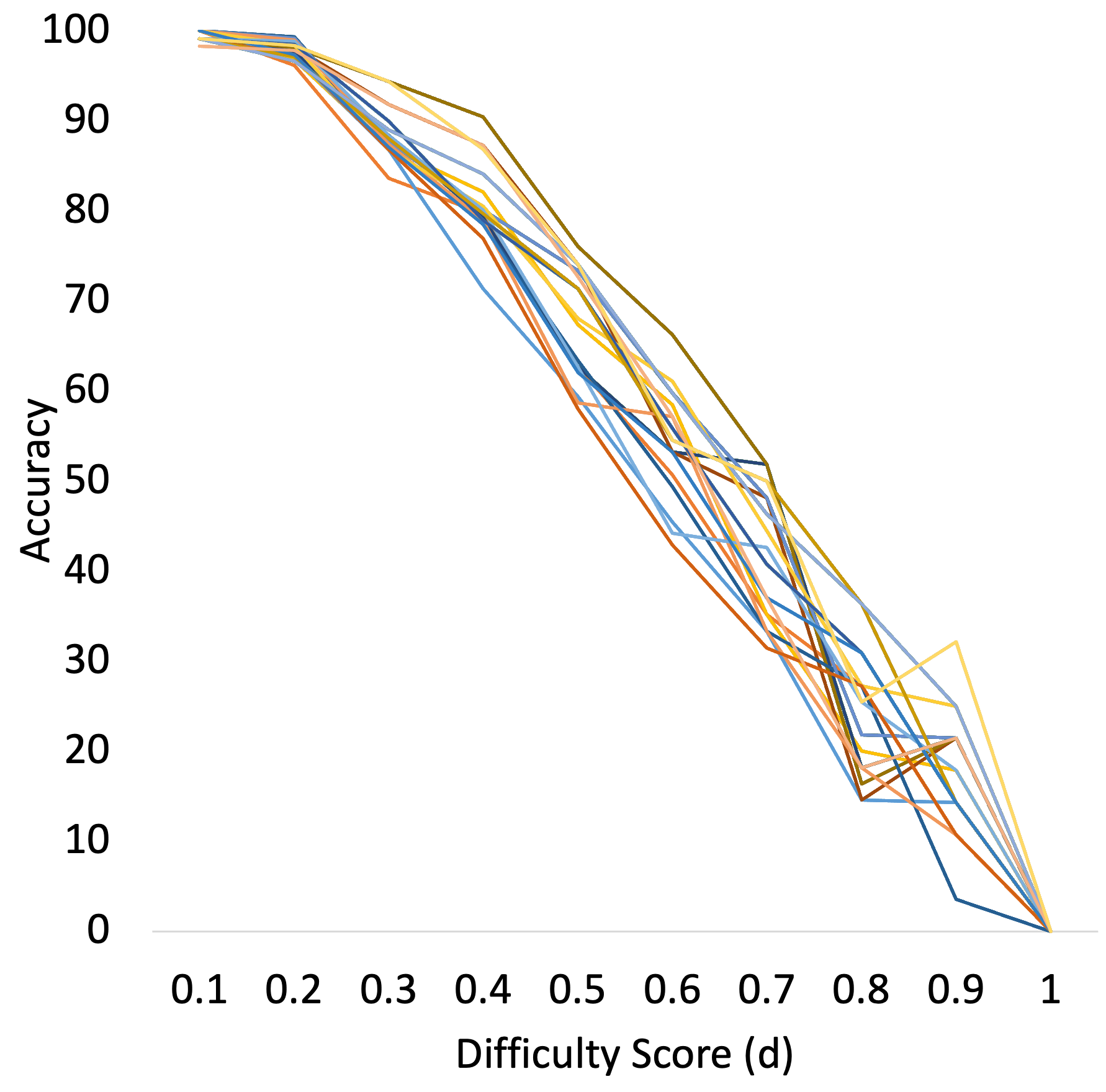
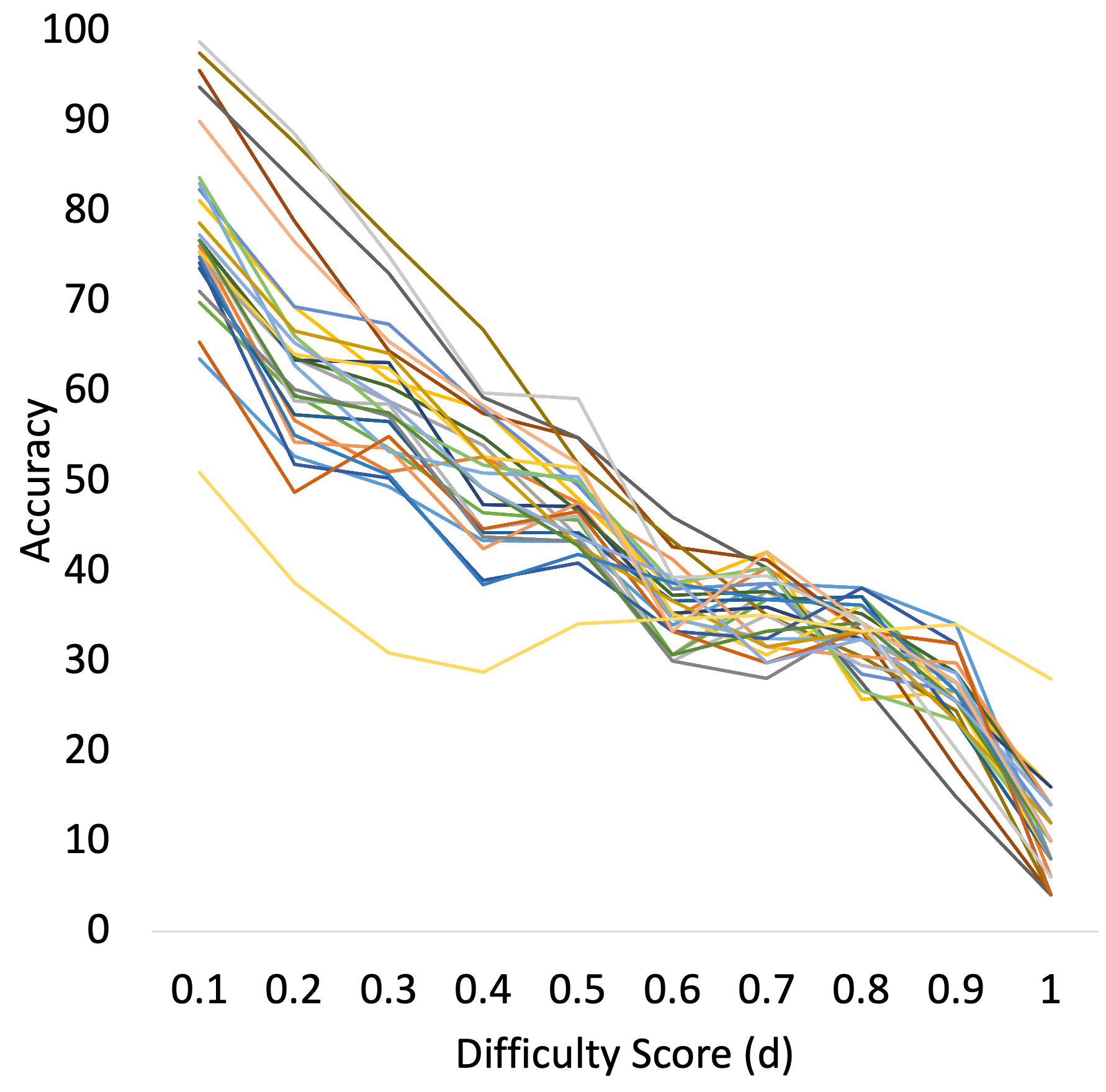
Figure 9 shows the trend of accuracy against difficulty scores for each individual model for MRPC and SocialIQA datasets.

Appendix B Datasets:

We experiment with the following datasets: SNLI Bowman et al. (2015), Multi-NLI Williams et al. (2018), Dialogue NLI Welleck et al. (2019), Adversarial NLI (R1, R2, R3) Nie et al. (2020), QNLI Wang et al. (2018), QQP Iyer et al. (2017), MRPC Dolan and Brockett (2005), PAWS-QQP, PAWS-Wiki Zhang et al. (2019), SST-2 Socher et al. (2013), COLA Warstadt et al. (2019) AG’s News Zhang et al. (2015), ARC-Easy, ARC-Challenge Clark et al. (2018), SWAG Zellers et al. (2018), Abductive-NLI Bhagavatula et al. (2020), Winogrande Sakaguchi et al. (2020), CommonsenseQA Talmor et al. (2019), QuaRel Tafjord et al. (2019a), QuaRTz Tafjord et al. (2019b), and SocialIQA Sap et al. (2019).

Appendix C Efficient Evaluations

Table 4 shows the Kendall correlation with full dataset evaluation achieved by our instance selection approach for different percentages of instances.

	25%	30%	40%	50%	60%	75%
Dataset	P	P	P	P	P	P
SNLI	$0.95_{0.0}$	$0.95_{0.01}$	$0.96_{0.01}$	$0.96_{0.01}$	$0.96_{0.01}$	$0.97_{0.01}$
PAWS Wiki	$0.98_{0.01}$	$0.98_{0.02}$	$0.98_{0.01}$	$0.98_{0.01}$	$0.98_{0.01}$	$0.99_{0.01}$
AgNews	$0.93_{0.01}$	$0.93_{0.02}$	$0.93_{0.01}$	$0.96_{0.01}$	$0.96_{0.01}$	$0.97_{0.01}$
QNLI	$0.92_{0.02}$	$0.92_{0.03}$	$0.93_{0.02}$	$0.96_{0.01}$	$0.96_{0.01}$	$0.97_{0.01}$
MRPC	$0.67_{0.13}$	$0.7_{0.11}$	$0.75_{0.08}$	$0.84_{0.05}$	$0.84_{0.03}$	$0.88_{0.03}$
SocialIQA	$0.84_{0.04}$	$0.87_{0.02}$	$0.89_{0.02}$	$0.91_{0.01}$	$0.93_{0.02}$	$0.94_{0.03}$
QQP	$0.96_{0.01}$	$0.96_{0.01}$	$0.96_{0.01}$	$0.97_{0.01}$	$0.98_{0.0}$	$0.99_{0.01}$
DNLI	$0.96_{0.02}$	$0.97_{0.02}$	$0.97_{0.02}$	$0.98_{0.01}$	$0.98_{0.01}$	$0.98_{0.01}$
COLA	$0.8_{0.05}$	$0.82_{0.07}$	$0.89_{0.06}$	$0.91_{0.02}$	$0.92_{0.04}$	$0.96_{0.02}$
SWAG	$0.97_{0.01}$	$0.96_{0.01}$	$0.97_{0.01}$	$0.98_{0.01}$	$0.99_{0.0}$	$0.99_{0.01}$
PAWS QQP	$0.89_{0.02}$	$0.92_{0.02}$	$0.92_{0.02}$	$0.93_{0.02}$	$0.94_{0.01}$	$0.94_{0.02}$
MNLI	$0.95_{0.01}$	$0.97_{0.01}$	$0.97_{0.01}$	$0.98_{0.0}$	$0.97_{0.01}$	$0.98_{0.01}$
Adv. NLI R1	$0.62_{0.06}$	$0.64_{0.08}$	$0.67_{0.06}$	$0.73_{0.06}$	$0.79_{0.05}$	$0.84_{0.07}$
Adv. NLI R2	$0.42_{0.08}$	$0.46_{0.1}$	$0.54_{0.14}$	$0.63_{0.05}$	$0.71_{0.05}$	$0.77_{0.03}$
Adv. NLI R3	$0.61_{0.05}$	$0.59_{0.06}$	$0.66_{0.1}$	$0.75_{0.06}$	$0.79_{0.06}$	$0.85_{0.04}$
SST-2	$0.83_{0.05}$	$0.86_{0.04}$	$0.87_{0.02}$	$0.87_{0.04}$	$0.91_{0.03}$	$0.92_{0.01}$
ARC Easy	$0.76_{0.07}$	$0.78_{0.08}$	$0.84_{0.08}$	$0.85_{0.05}$	$0.89_{0.03}$	$0.94_{0.02}$
ARC Diff	$0.41_{0.36}$	$0.49_{0.32}$	$0.62_{0.28}$	$0.59_{0.18}$	$0.75_{0.1}$	$0.86_{0.06}$
Abductive NLI	$0.72_{0.03}$	$0.77_{0.03}$	$0.79_{0.06}$	$0.82_{0.03}$	$0.86_{0.02}$	$0.88_{0.04}$
Winogrande	$0.24_{0.13}$	$0.3_{0.16}$	$0.39_{0.17}$	$0.44_{0.16}$	$0.53_{0.09}$	$0.63_{0.07}$
CSQA	$0.85_{0.04}$	$0.86_{0.03}$	$0.89_{0.03}$	$0.91_{0.02}$	$0.94_{0.02}$	$0.95_{0.01}$
QuaRel	$0.57_{0.12}$	$0.58_{0.16}$	$0.73_{0.1}$	$0.8_{0.15}$	$0.79_{0.07}$	$0.81_{0.07}$
QuaRTz	$0.37_{0.12}$	$0.44_{0.07}$	$0.51_{0.12}$	$0.57_{0.09}$	$0.62_{0.11}$	$0.64_{0.08}$

Table 4: Kendall correlation with full dataset evaluation achieved by our proposed instance selection approach for different percentage of instances. Each cell shows the mean and standard deviation obtained from 5 different runs.

Appendix D Actually Difficult Instances

Difficult Instance
Premise: Dog standing with 1 foot up in a large field. Hyp.: The dog is standing on one leg. Label: Contradiction.
Premise: A salt-and-pepper-haired man with beard and glasses wearing black sits on the grass. Hyp.: An elderly bearded man sitting on the grass. Label: Entailment.
Premise: A man is standing in front of a building holding heart shaped balloons and a woman is crossing the street. Hyp.: Someone is holding something heavy outside. Label: Contradiction.
Premise: A group of people plays a game on the floor of a living room while a TV plays in the background. Hyp.: A group of friends are playing the xbox while other friends wait for their turn. Label: Contradiction.

Table 5: Illustrative examples of instances that receive high difficulty score but are not erroneous. Such instances are difficult even for humans as they require reasoning ability.

Table 5 shows examples of instances that get assigned very high difficulty score but are actually difficult even for humans because they require reasoning abilities such as commonsense knowledge.

Appendix E Erroneous Instances

Dataset	Instance
SNLI	Premise: Trucks racing. Hyp.: Four trucks are racing against each other in the relay. Entailment, Neutral
(72%)	Premise: Two elderly men having a conversation. Hyp.: Two elderly woman having a conversation with their children. Neutral, Contradiction
CSQA	Why would a band be performing when there are no people nearby? O1: record album, O2: play music, O3: hold concert, O4: blaring, O5: practice
(50%)	What do audiences clap for? O1: cinema, O2: theatre, O3: movies, O4: show, O5: hockey game
WG	Maria was able to keep their weight off long term, unlike Felicia, because _ followed a healthy diet. O1: Maria, O2: Felicia
(36%)	When Derrick told Christopher about quitting school to provide for their family, _ started panicking. O1: Derrick, O2: Christopher
aNLI	O1: Ella was taking her final exam. O2: Ella was able to finish her exam on time. H1: Ella got to class early and was in no hurry. H2: Ella broke her pencil.
(x%)	O1: Cathy was happy that she finally had some time to sew. O2: Cathy tapped her metal fingertips on the table in frustration. H1: Cathy put the thimbles on. H2: Cathy could not get the thread into the fabric.

Table 6: Illustrative examples of erroneous instances in SNLI, CSQA, Winogrande, and Abductive NLI. Orange (ambiguous) and red (mislabeled) indicate the originally annotated answer while blue indicates the True/equally probable answer.

Table 6 shows examples of erroneous instances.

Appendix F Trivial Instances

Dataset	Instance
SNLI	Premise: A woman playing with her cats while taking pictures. Hyp.: A woman is playing with her dolls. Contradiction
CSQA	What will a person going for a jog likely be wearing? O1: grope, O2: acknowledgment, O3: comfortable clothes, O4: ipod, O5: passionate kisses
WG	Katrina did not value the antique pictures as much as Lindsey because _ was a history buff. O1: Katrina, O2: Lindsey
aNLI	O1: I bought a house with an ugly yard. O2: He carved the rock into a lion head and kept it. H1: There was a large rock in the yard. H2: I decided to tear the whole notebook up.

Table 7: Illustrative examples of trivial instances in SNLI, CSQA, Winogrande, and Abductive NLI. Text in blue corresponds to the ground-truth answer.

Table 7 shows examples of trivial instances.