Ill-posedness of degenerate dispersive equations
Abstract.
In this article we provide numerical and analytical evidence that some degenerate dispersive partial differential equations are ill-posed. Specifically we study the equation and the “degenerate Airy” equation . For our results are computational in nature: we conduct a series of numerical simulations which demonstrate that data which is very small in can be of unit size at a fixed time which is independent of the data’s size. For the degenerate Airy equation, our results are fully rigorous: we prove the existence of a compactly supported self-similar solution which, when combined with certain scaling invariances, implies ill-posedness (also in ).
1. Introduction
Dispersion plays a pivotal role in the analysis of the governing equations for a large number of physical phenomena, ranging from the evolution of surface water waves to the formation of Bose-Einstein condensates. A common theme in such problems is that uniform dispersive effects frequently control nonlinear terms which may otherwise lead to ill-posedness. Consider for instance the following class of quasilinear equations of KdV type studied in [8]:
| (1) |
where and . There it is shown that such equations are well-posed provided and . The first of these conditions guarantees that dispersive effects from do not vanish while the second prohibits the term from acting like a backwards heat operator. Similarly, the results on existence of solutions to the quasilinear dispersive equations found in [15] (about Schrödinger equations), [1] (water waves) and [29] (magma dynamics) share the feature that the dispersive effects are nondegenerate, to name just a few examples.
On the other hand, there are a number of physical problems in which the mechanism which causes the dispersive effects is not only nonlinear but degenerate. Some examples can be found in the study of sedimentation [26], shallow water [5], granular media [19, 11, 20], numerical analysis [14] and elastic rods and sheets [9, 16]. While there are a large number of articles in which degenerate dispersive equations (henceforth referred to as DDE) are derived [19, 20, 11, 5, 16, 9, 26], special solutions computed [24, 25, 11, 20, 19] or numerical computation of solutions performed [28, 27, 24, 10, 17, 6], the existence theory for the initial value problem of these equations is largely undeveloped.111The notable exception to this is the well-studied Camassa-Holm equation which when rewritten as a nonlocal evolution equation could be said to be degenerate and dispersive. This equation is integrable and consequently many results for it do not obviously generalize. The articles [10, 3, 13] prove some a priori estimates for DDE. [3] and [2] prove existence (but not uniqueness) of solutions to a very special class of DDE. [12] contains a semi-rigorous discussion of existence issues for these sorts of equations, including defining “-entropy solutions” by borrowing ideas from first order conservation laws. None of these articles fully settles the well-posedness issues for degenerate dispersion, and thus our interest is in studying the Cauchy problem for some simple and common DDE.
In particular we study the following two equations:
| (2) |
and
| (3) |
for . The first of these is the equation of Rosenau & Hyman [24]. Their goal was to understand the role of degenerate nonlinear dispersion in the formation of patterns and this equation (together with other members of the family ) has come to serve as the paradigm for degenerate dispersive systems. The most celebrated feature of this equation is the existence of compactly supported traveling waves, a.k.a. “compactons.” These are given by
where is the indicator function for the interval and . More recently, has been used to model pulses in both elastic and granular media [16, 21]. Equation (3), a “degenerate Airy equation”, appeared in [13] and is amongst the simplest equations which could be said to feature degenerate dispersion. We study it here due to its similarity to the equation and because it is of the form of (1) but does not meet the uniform dispersion hypothesis needed in [8].
Surprisingly, our conclusions are that both equations are ill-posed for data in . In particular, their solutions do not depend smoothly on their initial conditions. Our results for (2) are computational in nature: we conduct a series of numerical simulations of (2) which demonstrate that data which is very small in can be of unit size at a fixed time which is independent of the data’s size. For (3) our results are fully rigorous: we prove the existence of a compactly supported self-similar solution which, when combined with certain scaling invariances, implies ill-posedness. Note that our focus on initial data is due to the fact the compacton solutions of have a discontinuity in their second derivative at the edge of their support [18]. Consequently, they reside in but not , and so it is natural to work in this space.
Our suspicion that (2) is ill-posed has its origin in the various numerical simulations of collisions between compactons in equations. A wide variety of numerical methods has been used to compute solutions: pseudo-spectral [24], particle [6], Padé [28, 27], discontinuous Galerkin [17], and finite difference [10]. Each of these simulations shows that the computed collisions between compactons are nearly elastic: the compactons emerge from the collision nearly identical to their original state but phase shifted. As is common in collisions between solitary waves in “nearly” integrable PDE, the simulations show that in addition to the outgoing waves there is a small amplitude disturbance behind the waves. In nondegenerate problems, similar disturbances are sometimes called “dispersive ripples” and are viewed as being linear effects—the tail (approximately) solves the linearized equation [30, 31]. However, since the linearization of (2) about zero is trivial this heuristic cannot apply. The disturbance is described variously as: a compacton/anti-compacton pair in [24]; a numerical artifact in [28, 10]; and as a shock in [27]. No such disturbance is present at all in [6]. Lastly, the authors of [17] describe a “high-frequency oscillation” but go on to state “we do not know what is the source of these oscillations…” In each case, the qualitative features of the disturbance are quite different. Our feeling is that these discrepancies are not related to differences in the numerical methods or the implementation thereof but rather are due to an underlying issue with the equation itself.
Moreover, inspection of the right hand side of (2) provides evidence that the equation may be ill-posed. Observe that when , the term is formally a backwards heat operator. The key question, initially raised in [24], is this: can dispersive effects due to counteract the instability caused by the backwards heat operator ? Thus we should seek to understand the dispersive effects due to —hence our interest in (3). Our results show that the answer to the key question is “no”. As we stated above, our results show that is, in its own right, just as problematic as the backwards heat term. Differentiation of (3) with respect to yields for
Note that the second term on the RHS above is also a backwards heat operator when . The backwards heat term evident in (2) is, in this way, hidden in (3). Thus we expect blow up of when is negative. Moreover, this blow up should be particularly catastrophic when the function crosses the -axis with negative slope.
This motivates our approach: the self-similar solution constructed has such a transverse crossing and the resulting ill-posedness is due to blow up in the first and second derivatives of the solution. While our proof that (3) is ill-posed does not naturally carry over to (2), the numerics are highly suggestive. Most tellingly, since the numerics are performed using strictly positive initial data, they suggest the ill-posedness can manifest even in the absence of such a transverse crossing.
Remark 1.
In [7], Craig & Goodman demonstrate that the differential equation is ill-posed, whereas is not only well-posed but the solution map is essentially infinitely smoothing. The proofs of these facts follow from explicit formula for solutions of the initial value problems which can be constructed for each equation by mean of the Fourier transform and the method of characteristics.
The remainder of this paper is organized as follows. In Section 2 we show that the existence of a self-similar solution to (3) gives, as a consequence, the ill-posedness of the equation. In Section 3 we construct the self-similar solution using techniques from spatial dynamics. In Section 4 we discuss our numerical strategy for demonstrating ill-posedness of (2) and present the results of our simulations.
Acknowledgements: We would like to thank Professor Philip Rosenau for many interesting and helpful conversations regarding the degenerate dispersive equations studied in this article. Additionally, the work was supported by NSF Grants DMS 0926378, DMS 1008387, and DMS 1016267 (D.M.A.) and DMS 0908299 and DMS 0807738 (J.D.W.). G. S. was partially funded by NSERC. Finally, we are especially grateful the Louis and Bessie Stein Family Foundation who generously supported this work.
2. Self-similar solutions imply ill-posedness for (3)
We will prove there is a self-similar solution for (3) of the form
where gives the profile. Though other choices for the scaling are possible, we choose this particular set so that our proposed solution exhibits blow up (as ) in the first and second derivative while the norm remains bounded. Inserting this into (3) yields:
| (4) |
Here is the self-similar coordinate upon which depends and we have . We specify and so that the self-similar solution crosses the -axis transversely with negative slope, the “bad” situation identified in the Introduction.
We prove the following proposition concerning solutions of (4):
Proposition 1.
There exists , , and a function with the following properties:
-
(i)
solves (4) for all .
-
(ii)
, and .
-
(iii)
is negative in and has a unique minimum in the interior of this interval.
-
(iv)
.
-
(v)
for all sufficiently close to .
The proof of this proposition is technical and difficult and we postpone it until the next section. First we utilize it to prove our main result for (3):
Theorem 1.
The Cauchy problem for (3), posed in , does not depend smoothly on the initial data.
Proof.
(Theorem 1) The proof of the theorem is classical: we construct a sequence of solutions which are arbitrarily small in at but which are arbitrarily large when . Let
This is the profile function for our self-similar solution. See Figure 1.
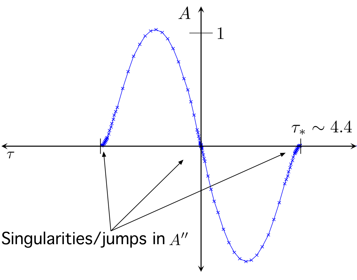
Note that it is compactly supported, not unlike the famous Barenblatt solution of the porous medium equation [4]. Also observe that is discontinuous at and diverges logarithmically at . Nevertheless, these singularities are sufficiently mild so that . Also observe that is continuous for all and consequently so is . Thus the function
is in fact a classical solution of (3). That is to say, while , is. Compare this with the compacton solution of : it is not in , though its square is.
For any and , (3) is invariant under the following transformation
| (5) |
Thus we have a two-parameter family of self-similar solutions of the form:
An elementary computation shows that
| (6) |
Fixing , setting and results in
(Here is a nonessential constant.) This pair of inequalities demonstrates that we have constructed a sequence of initial data for (3) which is arbitrarily small but whose solution at time is arbitrarily large. Thus the equation is ill-posed in .
∎
Remark 2.
In [13], the authors investigate self-similar solutions of the DDE . In particular they numerically compute profiles for shock and rarefaction solutions which are, in many respects, quite similar to the ones we find here. Namely, the shock solutions cross the -axis with negative slope and form a singularity in at the time of the shock formation. The solutions they find are not in —either they do not converge to zero as or their decay is not rapid enough to be integrable. Our focus here is on well-posedness issues in and consequently our strategies and methods will differ from those of [13].
3. Construction of the self-similar solution
This section is devoted to proving Proposition 1. We rewrite (4) as the initial value problem (IVP):
| (7) |
Our strategy will be as follows: first we will show that the IVP (7) has a unique solution, which depends on continuously. Next we will show that for sufficiently large the solution of (7) goes to zero in finite time. Then we will show that for there is a smallest time such that the solution of (7) has its first local maximum at and remains strictly negative for all . See Figure 2.
Then an open/closed argument will give the special solution for a choice .
The differential equation (4) is nonlinear, nonautonomous and singular at . As such, carrying out the details of our strategy is quite challenging. The key observation for proving Proposition 1 is that (4) is, in a loose sense, close to being hamiltonian. Specifically, one can rewrite the right hand side of (4) as . If we then consider the related equation
| (8) |
obtained from (4) by replacing the nonautonomous with the constant , one sees that this equation is in fact hamiltonian. Specifically one can integrate both sides to find:
The conserved energy is
and most of the dynamics of (8) can be determined by analyzing this quantity. In the following proof of Proposition 1, we will frequently make use of quantities similar to this energy which, though not conserved for solutions of (4), do provide quite a bit of dynamical information about solutions.
3.1. Well-posedness of (7)
Now we prove (7) has unique solutions and that such solutions depend smoothly upon .
Lemma 2.
Proof.
Letting , (4) can be written as . If were continuous in and Lipschitz in throughout a neighborhood of , then Lemma 2 would be a trivial consequence of the standard theory on existence and uniqueness of solutions and their continuous dependence on initial conditions. Unfortunately, in our case is not even defined if . However, notice that if there exists a solution to the IVP (7) then L’Hopital’s rule implies:
Therefore our strategy will be to remove the singularity at by modifying in such a way that the resulting modification is continuous in a neighborhood of the initial data and agrees with for solutions of .
Fix and , and let
Given the initial conditions in (7), and formally give crude lower and upper bounds on for close to . Now construct the following function:
is well-defined and continuous throughout a small neighborhood of for any . Then we have the existence of a solution to the IVP:
Furthermore, it is easy to verify that there exist and such that for each the solution is defined for all and satisfies for all . It follows that the restriction of to is in fact a solution to the IVP (7).
Note that along any solution of (7), as . Consequently, it is not possible to modify to a function that is Lipschitz in in a neighborhood of . Therefore, we have to establish the uniqueness of the solution by other means, namely the nearly hamiltonian structure of (4).
For any , let and be solutions to the IVP (7) with and , respectively. Recall that our choice of and ensures for all . Thus we can take a sufficiently small , independent of and , such that for all and
Then for any ,
| (9) |
where the equalities hold if .
Since both and are solutions to the ODE, we have
Integrating the above equation gives
where . Then by incorporating (9), we obtain that for all ,
| (10) |
Together with the initial conditions and , (10) implies that for all ,
Recall . It follows that for all ,
By the definition of , we have , which implies
| (11) |
When (i.e., ), Inequality (11) requires . Consequently, for all . This proves the uniqueness of the solution on the interval . Recall that with , for all by our choice of and . Then with the initial conditions , , constitutes a regular initial value problem, to which is the unique solution throughout the interval according to the standard existence and uniqueness theory. Altogether, we have shown the uniqueness of the solution on the full interval .
Since the choice of is independent of and , after combining (10) and (11) and integrating we can obtain a uniform constant such that for any ,
for all . Since for all , by applying Gronwall’s inequality on the interval we can extend the above inequality to the full interval after replacing with some larger . ∎
Let be the solution to the IVP (7) with . Clearly, we can extend to any as long as for all . Furthermore, by considering with the initial conditions specified at and set close to , we can extend Lemma 2 to the interval . In particular, by applying Gronwall’s inequality on the interval , we obtain the following corollary.
Corollary 3.
For any such that for all , there exist and a sufficiently small such that for any the solution with remains negative for all and satisfies
| (12) |
for all .
3.2. General behavior of solutions
Now that we know (7) is well-posed, we demonstrate some properties of solutions when . First, its solutions reach a first minimum in finite time. Let
| (13) |
Note that depends upon , though we supress this for notational simplicity.
Lemma 4.
For any we have . In addition, and . Moreover there exist such that implies (a) , (b) and (c) .
Proof.
Clearly, if is finite. For (possibly ), and are negative and consequently . Thus is increasing. This implies that for and also if is finite. Thus is concave up on . This together with the fact that implies via the mean value theorem that for all and so . Thus we have
| (14) |
for . Integrating this inequality twice gives for all . If , the lower bound on becomes positive in finite time, implying that . Examination of the zeroes of the upper and lower bounds gives the estimates for stated in the lemma. Further integration of (14) gives the estimates on and . If , the lower bound on is not sufficient to conclude that . However the fact that can be used to improve the lower bound in this case. The details are standard and omitted.
∎
After reaching their first local minimum at , solutions either reach zero in finite time or alternately reach a local maximum (for which ) in finite time, as we now demonstrate. Let
| (15) |
As with , implicitly depends upon . If this is finite, then we have either and or and .
Lemma 5.
For all we have
Proof.
Clearly since . Suppose that . Since is bounded above and nondecreasing for , we have convergent as . Since we have and for all , (7) implies for all as well. Thus is nonincreasing. Since it is initially positive and converges, clearly must eventually become negative. Since is nonincreasing, once it is negative it remains negative for all subsequent times. Thus there is an and a value such that for all . Integrating this, however, indicates that must eventually become negative, a contradiction, and the lemma is shown. ∎
3.3. Energy estimates and behavior of for or large
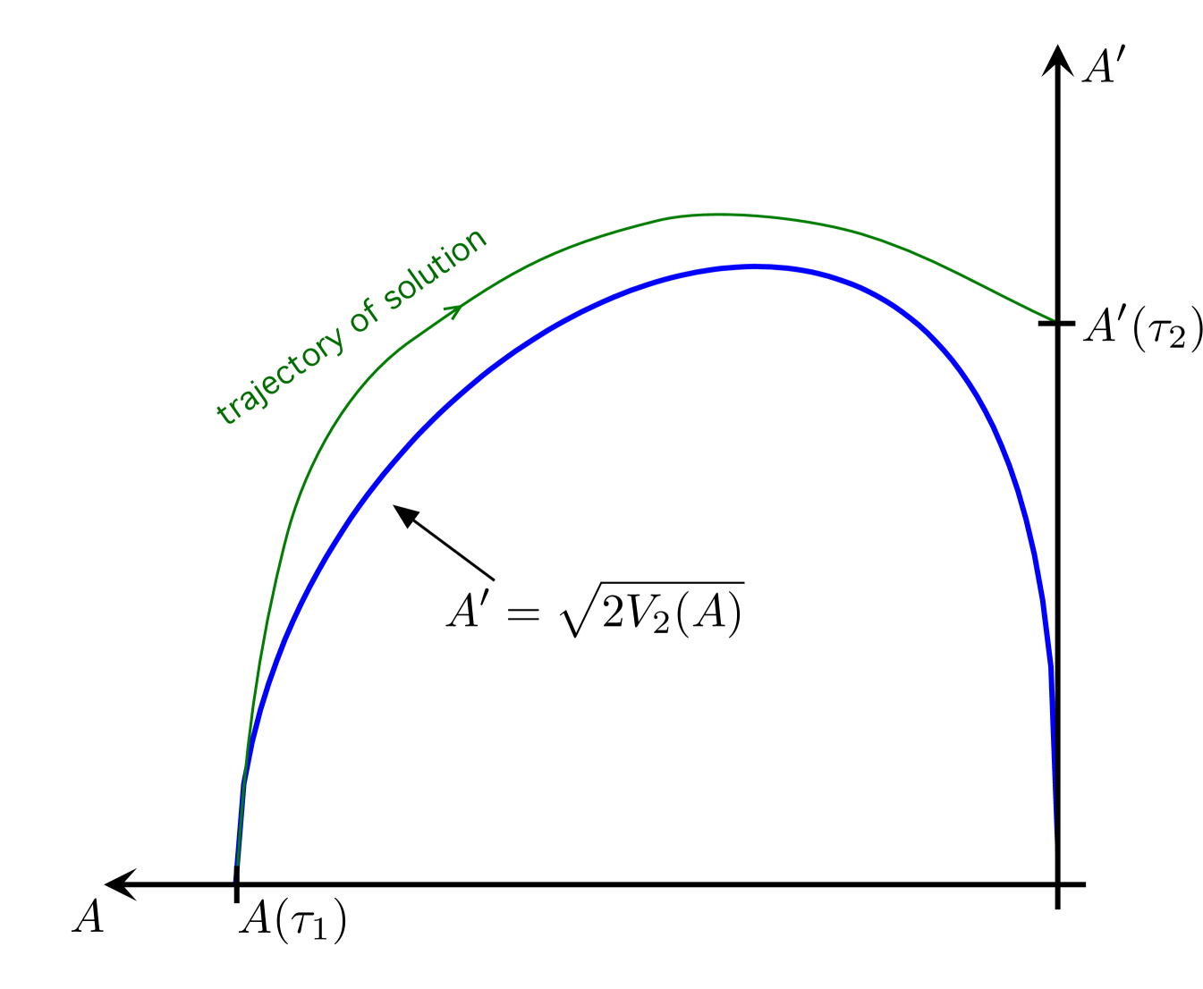
Our next goal is to show that for large, solutions go to zero in finite time but when the solution has a local negative maximum at . This requires the following energy estimates, similar to those for (8):
Lemma 6.
Fix and take and as above. Let
Then for all
Moreover, take and set
If then for all
Proof.
Let . By definition of , we have and for all . If then we have for all ,
where the equalities hold only if and the second inequality is true independent of . Integrating this from to gives
for all . Note that we obtain strict inequalities here because with there is a small such that for all . If we multiply by and integrate once more from to any then the conclusions of the lemma follow. In particular, is irrelevant to the upper bound . ∎
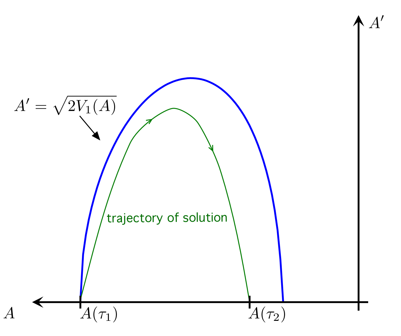
Lemma 7.
There exists such that implies and .
Proof.
First we show that if then we are done. We know by the definition of that either or . Inspection of demonstrates that for and is zero at the ends of that interval (see Figure 3). Thus, since is increasing on we have and therefore . We also know for that . So in particular Lemma 6 implies . So, since it must be the case that .
On the other hand perhaps . We will prove by contradiction that this is impossible when is large. The estimate in the proof of Lemma 6 gives:
which is valid for if we assume . (Note that for big enough, the estimates on in Lemma 4 imply that .) Integration from to gives
Substitution in from the definition of and gives
A change of variables and the fact that implies:
Letting we have
Now we employ the estimates in Lemma 4 to find for all :
For sufficiently large this is impossible and so the lemma is shown.
∎
Lemma 8.
If , then and .
Proof.
Proving the lemma amounts to showing that . Notice that . Let . , since . Also . In the proof of Lemma 4 we saw that for (see (14)) and so . Consequently . Thus, since , we have Moreover, and . Thus there is a point at which . See Figure 4.
Since for we have and we must therefore have . Since is finite for and is bounded from zero for all , the definition (15) of requires .
∎
3.4. Openness of qualitative behavior
The next pair of results show that slightly varying does not change the qualitative behavior of at . That is to say, if is such that then there is an open neighborhood of where the corresponding solutions enjoy this same property. Likewise, if such that , then there is an open neighborhood of where the corresponding solutions do the same. Let be the solution to the IVP (7) with , and define for as in (15).
Lemma 9.
Suppose and . Then for any there exists a such that for any , the solution to the IVP (7) with reaches zero at .
Proof.
Since , the right hand side of (4) is undefined at this point and so we cannot directly use our results about continuous dependence on from Corollary 3 to prove this result. Instead we will have to rely instead on the nearly hamiltonian structure of (4).
Integrating the ODE of (7) with the initial conditions , , and , we obtain that
| (16) |
as long as on the interval .
Since and , we can choose a small such that and for all . It follows that
Therefore, as . Applying (16) to and taking the limits of both sides as , we obtain
Suppose there exist an and a sequence such that for any , the solution to the IVP (7) with is below zero for all . Since for all , we can apply (12) of Corollary 3 to obtain a subsequence and some such that for each ,
for all . Clearly, . Without loss of generality, we assume that for all . Let
Note that as . Otherwise, for some very large , would reach zero at some since converges to from below. Without loss of generality, we assume that for all . Then the definition of implies and for all . Applying (16) to at yields
Since , the right-hand side converges to . However, for all the left-hand side is greater than or equal to . This is a contradiction. ∎
In the next lemma, we still assume .
Lemma 10.
Suppose and . Then there exists a such that for any , the solution to the IVP (7) with satisfies and .
Proof.
Define for as in (13). Then since . It follows that and for all . Thus there is a such that . Furthermore, since for all , we have . This allows us to choose a small such that for all , , and . Take a small . Then Corollary 3 guarantees the existence of a such that for any , the solution with is below zero for all and satisfies and . This implies that and at . ∎
3.5. Final steps
We are now in a position to complete the proof of Proposition 1.
Proof.
Define the set as follows:
Lemma 7 guarantees that is nonempty, and Lemma 8 shows that zero is a lower bound of . Take , with the inequality guaranteed by Lemma 8 and Lemma 10. Let be the solution to the IVP (7) with . Then by Lemma 9 and the definition of , it is only possible that either and or and . Furthermore, we rule out the second case by the definition of and Lemma 10. This proves (i)–(iv) of Proposition 1.
Since and for all , we have
for all . Integrating the above inequality gives
for all . Thus as . Then we can take a sufficiently small such that for all . By the mean value theorem we have
for any and some . Since , this implies that and consequently for all . Thus as . This proves (v) of Proposition 1.
∎
4. Numerical Study of
4.1. Regularization and scaling
In this section we numerically assess the ill-posedness of (2). But it is inappropriate to directly simulate an equation that not only lacks a local well-posedness theory but for which we suspect ill-posedness. Thus we regularize the equation. Simulating this regularized problem, we find evidence of the ill-posedness as we let the regularization parameter vanish.
We study the following regularization of (2)
| (17) |
Here is the identity and is the small regularization parameter. We choose this particular regularization since its implementation is natural when simulating solutions of (2) via a pseudospectral method.
Inverting the operator on the left-hand side to be able to write it as an evolution equation, we see that and are bounded operators. Indeed,
The boundedness of these operators make it trivial to prove:
Theorem 11 (Local Well-Posedness of a Regularized Problem).
The proof of this, which we omit, is an elementary application of the fixed point technique. The operator is bounded in -based Sobolev spaces. For , is an algebra which makes the nonlinearity easy to treat. An impediment to extending Theorem 11 to one which is global in time, or even one which holds on time intervals of a length uniform in , is the lack of an obvious coercive conserved quantity associated with (17). The only obvious conserved quantity for (17) is
This is formally an invariant for solutions of as well.
By simulating the regularized equation (17) we seek evidence of ill-posedness of (2). In particular, we shall find a sequence of vanishing initial conditions for (17), such that as , the corresponding solutions at have norm of (at least) unit size. To that end, we will scale the initial data for (17) using the same scaling given by (5) and link the vanishing of the smoothing parameter to the scaling parameter . Specifically we will study (17) with
| (18) |
where
and . Note that the calculations leading to (6) show that and so this choice of initial data vanishes in the limit. We denote the solution of (17) with the choices in (18) by . Note that we have taken our initial data to be everywhere positive, unlike the self-similar solutions found for (3). We do this to demonstrate that the problematic effects of degeneracy manifest themselves even for solutions which do not cross the -axis.
The choices for and are made for the following reason. Instead of scaling just the initial data for (17) suppose that we rescale the whole equation by
| (19) |
Then (17) becomes:
where . Plugging in from (18) we get
and
| (20) |
Of course (20) is not an exact scaling. Notice that as the term term will vanish. The equation will asymptotically be dominated by the third derivative term which is consistent with our expectation that this term is the source of the ill-posedness. Moreover notice that the coefficient of regularization even in these scaled coordinates vanishes. That is to say, we have chosen the regularization parameter so that it vanishes “more rapidly” than scaling effects.
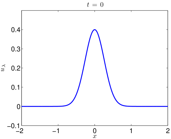
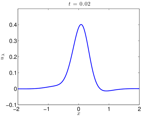
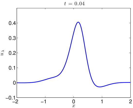
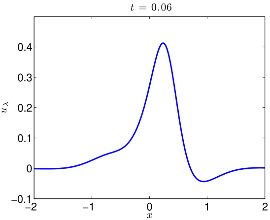
4.2. Computational results
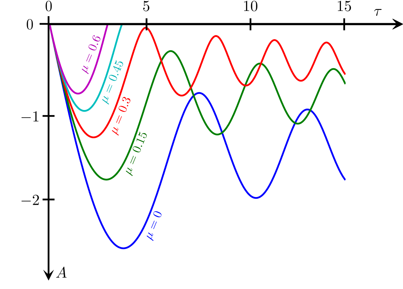
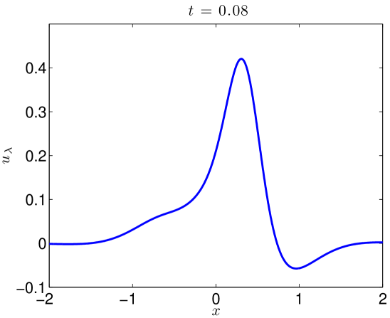
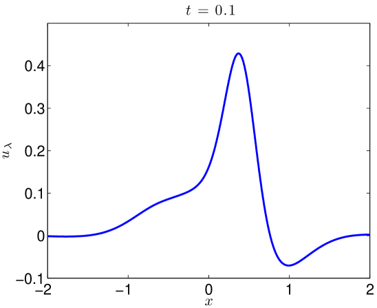
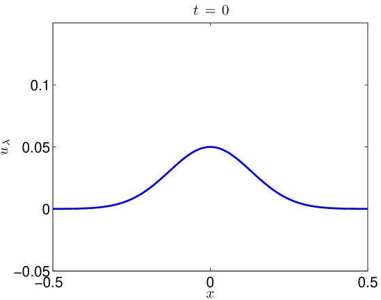
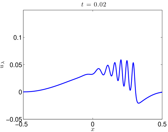
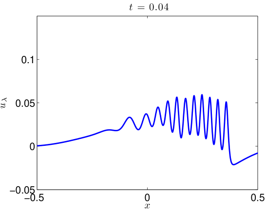
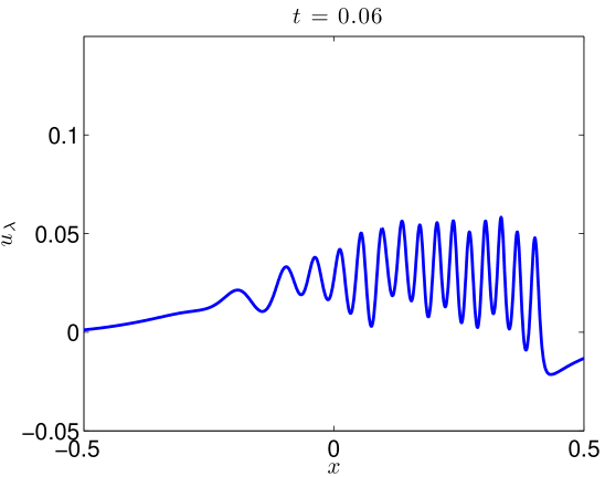
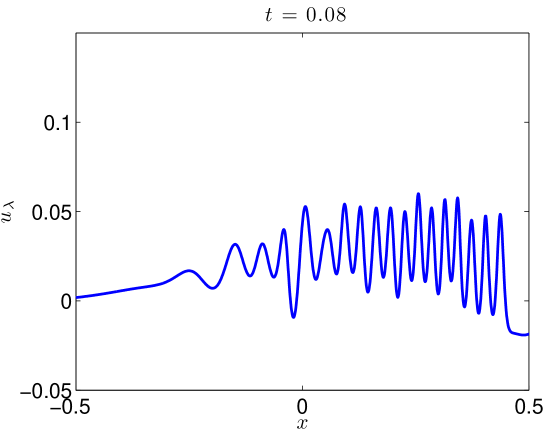
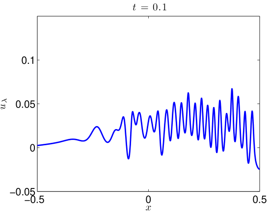
We integrate our problem pseudospectrally with a Crank-Nicholson time stepping scheme. Some additional details are presented in Section 4.3. Simulating (17) with (18) to on the domain with resolved Fourier modes, the data evolves as in Figures 5 and 6. At large values of , there is some development of oscillations. At very small values of , it develops a highly oscillatory structure. Note that these oscillations appear for , where . That is to say in the exactly the place where the term in (2) acts, heuristically, as a backwards heat operator.
We present the evolution of the , , and norms in Figure 7 of the solutions as functions of time. Though there is little growth in time of the norm, we see orders of magnitude jumps in the and norms at as we send .
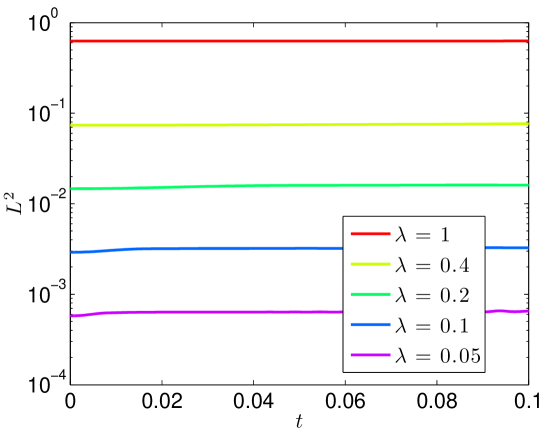
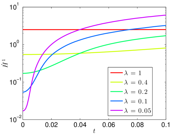
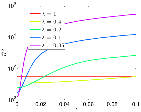
We contend that this is evidence of ill-posedness. We have a sequence of initial conditions , which have vanishing norm. At a fixed , the norms are growing as we let . Thus, there is a loss of continuous dependence of the solution map upon the initial data about the solution.
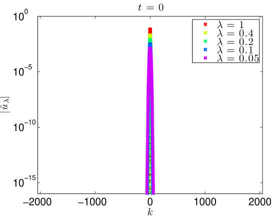
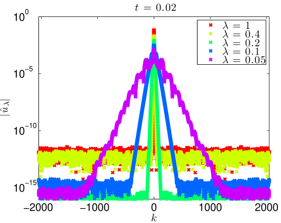
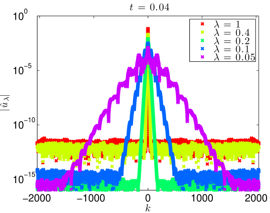
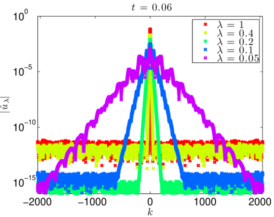
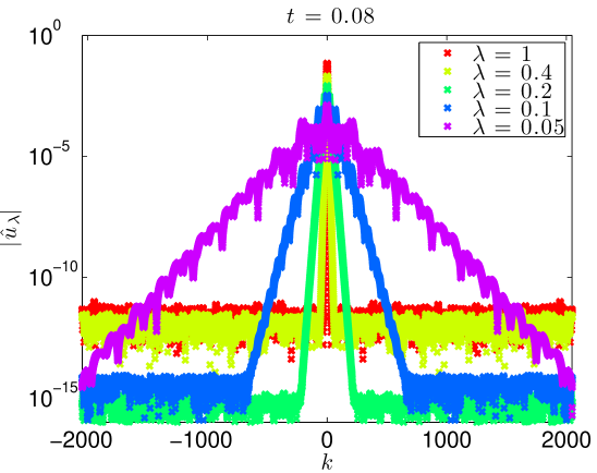
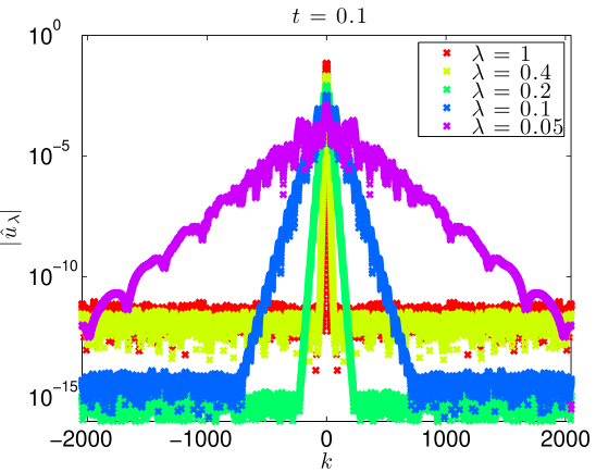
This growth in the norm corresponds to a spreading in Fourier space. Indeed, Figure 8 shows precisely this. At fixed time, the Fourier support grows as . These figures also indicate that except for , all simulations are extremely well resolved. Even the simulation is well resolved through , and only slightly under resolved at the final time, .
4.3. Details of numerical methods
As noted, the simulations presented in Section 4 were generated using a fully de-aliased pseudospectral discretization with Crank-Nicholson time stepping. This was performed in Matlab and fsolve was used to solve the nonlinear system at each time step with a tolerance of . 8192 modes were resolved in these simulations, with a time step of .
The invariant was conserved to at least eight significant figures in all the computed cases, as shown in Table 1.
| 1 | 0.4 | 0.2 | 0.1 | 0.05 | ||
|---|---|---|---|---|---|---|
| 0.00 | 0.886226925453 | 0.261191032665 | 0.103653730004 | 0.0411350100123 | 0.0163244395416 | |
| 0.02 | 0.886226925477 | 0.261191032667 | 0.103653730004 | 0.0411350100123 | 0.0163244395416 | |
| 0.04 | 0.886226925489 | 0.261191032674 | 0.103653730004 | 0.0411350100123 | 0.0163244395416 | |
| 0.06 | 0.886226925478 | 0.261191032676 | 0.103653730004 | 0.0411350100123 | 0.0163244395416 | |
| 0.08 | 0.886226925497 | 0.261191032673 | 0.103653730004 | 0.0411350100123 | 0.0163244395416 | |
| 0.10 | 0.886226925509 | 0.261191032673 | 0.103653730004 | 0.0411350100123 | 0.0163244395416 | |
4.4. Convergence of Norms
Since we are concerned with the value of at the end of our simulation, it is also important to confirm that this is converging to a fixed value as we refine the spatial and temporal resolution of our simulations. For the initial condition with , Table 2 gives the values of the norm for various choices of the number of resolved Fourier modes, , and the time step, . With only 512 resolved modes, we appear to be fully resolved in space, and there is little gain in accuracy when is increased. Of course, for other initial conditions, more than 512 modes may be needed to resolve the simulation.
| 0.004 | 0.002 | 0.001 | ||
|---|---|---|---|---|
| 512 | 675.27623578 | 692.22147559 | 696.5301160 | |
| 1024 | 675.27623585 | 692.22147576 | 696.5301162 | |
| 2048 | 675.27623587 | 692.22147576 | 696.5301162 | |
| 4096 | 675.27623586 | 692.22147576 | 696.5301162 | |
| 8192 | 675.27623586 | 692.22147576 | 696.5301162 | |
For the three values of , we appear to have achieved at least one significant digit of accuracy and as we reduce the time step, the variations of become smaller. Since we are using a Crank-Nicholson scheme, we expect convergence. If we perform Richardson extrapolation, the estimated value of based on the and simulations is 697.87. Comparing the and simulations, the estimated value is 697.97. Separate computations, performed with just 512 grid points for expediency, show that with the norm takes the value 697.96, and for , the value is 697.99.
An examination of the case is similar. For the same three values of , the norms, given in Table 3, are in agreement on the order of magnitude. Richardson extrapolation using the data at and predicts a value of 15148, while the predicted value based on the and value is 15278. Independent simulations with 2048 grid points yield a value of 15253 when and a value of 15302 when . Thus, we believe that our choice of discretization parameters, and , for the results presented in Section 4.2 yield meaningful measurements of that are accurate to at least one signfigant figure. This is sufficient for our study of ill-posedness.
| 0.004 | 0.002 | 0.001 | ||
|---|---|---|---|---|
| 2048 | 12452.791732 | 14474.328299 | 15077.20691 | |
| 4096 | 12452.791732 | 14474.328298 | 15077.20691 | |
| 8192 | 12452.791732 | 14474.328299 | 15077.20691 | |
References
- [1] D. M. Ambrose and N. Masmoudi. Well-posedness of 3D vortex sheets with surface tension. Commun. Math. Sci., 5(2):391–430, 2007.
- [2] D. M. Ambrose and J. D. Wright. Traveling waves and weak solutions for an equation with degenerate dispersion. Preprint.
- [3] D. M. Ambrose and J. D. Wright. Preservation of support and positivity for solutions of degenerate evolution equations. Nonlinearity, 23(3):607–620, 2010.
- [4] G. I. Barenblatt. On self-similar motions of a compressible fluid in a porous medium. Akad. Nauk SSSR. Prikl. Mat. Meh., 16:679–698, 1952.
- [5] R. Camassa and D. D. Holm. An integrable shallow water equation with peaked solitons. Phys. Rev. Lett., 71(11):1661–1664, 1993.
- [6] A. Chertock and D. Levy. Particle methods for dispersive equations. J. Comput. Phys., 171(2):708–730, 2001.
- [7] W. Craig and J. Goodman. Linear dispersive equations of Airy type. J. Differential Equations, 87(1):38–61, 1990.
- [8] W. Craig, T. Kappeler, and W. Strauss. Gain of regularity for equations of KdV type. Ann. Inst. H. Poincaré Anal. Non Linéaire, 9(2):147–186, 1992.
- [9] H.-H. Dai and Y. Huo. Solitary shock waves and other travelling waves in a general compressible hyperelastic rod. R. Soc. Lond. Proc. Ser. A Math. Phys. Eng. Sci., 456(1994):331–363, 2000.
- [10] J. de Frutos, M. Á. López Marcos, and J. M. Sanz-Serna. A finite difference scheme for the compacton equation. J. Comput. Phys., 120(2):248–252, 1995.
- [11] F. Fraternali, M. A. Porter, and C. Daraio. Optimal Design of Composite Granular Protectors. Mech. Adv. Mater. Struct., 17(1):1–19, 2010.
- [12] V. A. Galaktionov. Nonlinear dispersion equations: smooth deformations, compactions, and extensions to higher orders. Zh. Vychisl. Mat. Mat. Fiz., 48(10):1859, 2008.
- [13] V. A. Galaktionov and S. I. Pokhozhaev. Third-order nonlinear dispersion equations: shock waves, rarefaction waves, and blow-up waves. Zh. Vychisl. Mat. Mat. Fiz., 48(10):1819–1846, 2008.
- [14] J. Goodman and P. D. Lax. On dispersive difference schemes. I. Comm. Pure Appl. Math., 41(5):591–613, 1988.
- [15] C. E. Kenig, G. Ponce, and L. Vega. The initial value problem for the general quasi-linear Schrödinger equation. In Recent developments in nonlinear partial differential equations, volume 439 of Contemp. Math., pages 101–115. Amer. Math. Soc., Providence, RI, 2007.
- [16] D. Ketcheson. High Order Strong Stability Preserving Time Integrators and Numerical Wave Propagation Methods for Hyperbolic PDEs. 2009.
- [17] D. Levy, C.-W. Shu, and J. Yan. Local discontinuous Galerkin methods for nonlinear dispersive equations. J. Comput. Phys., 196(2):751–772, 2004.
- [18] Y. A. Li, P. J. Olver, and P. Rosenau. Non-analytic solutions of nonlinear wave models. In Nonlinear theory of generalized functions (Vienna, 1997), volume 401 of Chapman & Hall/CRC Res. Notes Math., pages 129–145. Chapman & Hall/CRC, Boca Raton, FL, 1999.
- [19] V. F. Nesterenko. Dynamics of hetereogeneous materials. Springer, New York, NY, 2001.
- [20] L. Ponson, N. Boechler, Y. M. Lai, M. A. Porter, P. G. Kevrekidis, and C. Daraio. Nonlinear waves in disordered diatomic granular chains. Phys. Rev. E, 82(2, Part 1), AUG 12 2010.
- [21] M. Porter, C. Daraio, I. Szelengowicz, E. Herbold, and P. Kevrekidis. Highly nonlinear solitary waves in heterogeneous periodic granular media. Physica D, 2009.
- [22] P. Rosenau. Nonlinear dispersion and compact structures. Phys. Rev. Lett., 73(13):1737–1741, 1994.
- [23] P. Rosenau. Compact and noncompact dispersive patterns. Phys. Lett. A, 275(3):193–203, 2000.
- [24] P. Rosenau and J. Hyman. Compactons: solitons with finite wavelength. Phys. Rev. Lett., (70):564–567, 1993.
- [25] P. Rosenau and E. Kashdan. Emergence of compact structures in a klein-gordon model. Phys. Rev. Lett., (104), 2010.
- [26] J. Rubinstein and J. B. Keller. Sedimentation of a dilute suspension. Phys. Fluids A, 1(4):637–643, 1989.
- [27] F. Rus and F. R. Villatoro. Padé numerical method for the Rosenau-Hyman compacton equation. Math. Comput. Simulation, 76(1-3):188–192, 2007.
- [28] F. Rus and F. R. Villatoro. Self-similar radiation from numerical Rosenau-Hyman compactons. J. Comput. Phys., 227(1):440–454, 2007.
- [29] G. Simpson, M. Spiegelman, and M. I. Weinstein. Degenerate dispersive equations arising in the study of magma dynamics. Nonlinearity, 20(1):21–49, 2007.
- [30] C. E. Wayne and J. D. Wright. Higher order modulation equations for a Boussinesq equation. SIAM J. Appl. Dyn. Syst., 1(2):271–302 (electronic), 2002.
- [31] J. D. Wright. Higher order corrections to the KdV approximation for water waves. ProQuest LLC, Ann Arbor, MI, 2004. Thesis (Ph.D.)–Boston University.