Image-Constrained Modeling with Hubble and Keck Images Reveals that OGLE-2012-BLG-0563Lb is a Jupiter-Mass planet Orbiting a K Dwarf
Abstract
We present high angular resolution imaging from the Hubble Space Telescope combined with adaptive optics imaging results from the Keck-II telescope to determine the mass of the OGLE-2012-BLG-0563L host star and planet to be and , respectively, located at a distance of kpc. There is a close-wide degeneracy in the light curve models that indicates star-planet projected separation of AU for the close model and AU for the wide model. We used the image-constrained modeling method to analyze the light curve data with constraints from this high angular resolution image analysis. This revealed systematic errors in some of the ground-based light curve photometry that led to an estimate of the angular Einstein Radius, , that was too large by a factor of . The host star mass is a factor of 2.4 larger than the value presented in the Fukui et al. (2015) discovery paper. Although most systematic photometry errors seen in ground-based microlensing light curve photometry will not be repeated in data from the Roman Space Telescope’s Galactic Bulge Time Domain Survey, we argue that image constrained modeling will be a valuable method to identify possible systematic errors in Roman photometry.
1 Introduction
The gravitational microlensing exoplanet detection method plays a key role in understanding the exoplanet population in our Galaxy, despite the fact that the method was introduced only 33 years ago (Mao & Paczynski, 1991) and its sensitivity to low-mass planets was only recognized 28 years ago (Bennett & Rhie, 1996). Microlensing’s unique sensitivity to low-mass planets in orbits wider than the Earth’s orbit has led NASA to include a space-based microlensing exoplanet survey (Bennett & Rhie, 2002) as a key observing program that will use large fraction of the observing time for the Nancy Grace Roman Space Telescope (Bennett et al., 2010a, 2018a; Spergel et al., 2015; Penny et al., 2019).
A somewhat attractive feature of the microlensing method is that it is able to detect planets without detecting any light from their host stars. This has enabled microlensing to detect the first Jupiter-like planet in a Jupiter-like orbit around a white dwarf (Blackman et al., 2021). It has also enabled the discovery of planets with no evidence for any host star (Mróz et al., 2018, 2019, 2020a; Ryu et al., 2021; Kim et al., 2021; Koshimoto et al., 2023), implying that they are likely to be unbound from any host star, although some could certainly be in wide orbits about host stars. Two of these candidate free-floating planets are likely to have masses slightly lower than an Earth-mass (Mróz et al., 2020b; Koshimoto et al., 2023), and a statistical analysis implies that these planets are likely to be times more common than the known populations of bound planets (Sumi et al., 2023).
However, the lack of clear detection of light from the planetary host star can be a problem for planetary microlensing events with main sequence host stars. Methods of characterizing the physical properties of planetary microlens systems, such as masses, distance, and orbital separation, have been discussed by Bennett et al. (2007). In some cases it is possible to determine the masses and distances with light curve data alone if both the angular Einstein radius, , and the amplitude of microlensing parallax, , are both measured. However, this is possible for only a fraction of events, usually with a bright source star and a duration long enough to see the effects of the Earth’s orbital motion in the light curve (e.g. Muraki et al., 2011) or observations by a telescope in a Heliocentric orbit (e.g. Street et al., 2016).
Of the 29 events, with 30 planets, in the Suzuki et al. (2016) sample (hereafter S16), only three MOA-2009-BLG-266 (Muraki et al., 2011), MOA-2010-BLG-117 (Bennett et al., 2018a) and OGLE-2011-BLG-0265 (Skowron et al., 2015), have been characterized with mass measurements using only light curve data. These three events provided measurements of and that were precise enough to determine the host star and planet masses. High angular resolution follow-up observations have been used to characterize almost all of the other 26 S16 sample events. The only exceptions are 4 events with giant source stars, which make it very difficult to detect the host stars with high angular resolution follow-up images, although two of the giant source star events, MOA-2009-BLG-266 and OGLE-2011-BLG-0265 were characterized with and measurements. Excluding the events with giant source stars and the third event characterized with light curve measurements of and (MOA-2010-BLG-117), we are left with 22 events that we attempted to characterize with high angular resolution observations with the the Hubble Space Telescope and/or Keck Telescope adaptive optics (AO) imagers. Of these 22 events, we have detected the host stars for 13 events, although in the case of the “ambiguous” event of the S16 sample, the host star detection confirmed the non-planetary, stellar binary model (Terry et al., 2022). The planetary host stars were detected for OGLE-2005-BLG-071, OGLE-2005-BLG-169, OGLE-2006-BLG-109, MOA-2007-BLG-192, MOA-2007-BLG-400, OGLE-2007-BLG-349, MOA-2008-BLG-379, OGLE-2008-BLG-355, MOA-2009-BLG-319, MOA-2010-BLG-328, MOA-2011-BLG-262, OGLE-2012-BLG-0950, and the event discussed in this paper, OGLE-2012-BLG-0563 (Batista et al., 2015; Bennett et al., 2010, 2015, 2016, 2020, 2024; Bhattacharya et al., 2018, 2021; Gaudi et al., 2008; Terry et al., 2021, 2024). The papers on 3 of these events are still under preparation. There are also two events without host star detections despite very good high angular resolution follow-up data. (Bhattacharya et al., 2017) found that a candidate host star identified in the discovery paper (Janczak et al., 2010), was actually a star that was unrelated to the microlensing event, and Keck images taken by Blackman et al. (2021) ruled out main sequence stars, while microlensing parallax limits from the light curve data (Bachelet et al., 2012) ruled out brown dwarf, neutron star, and black hole hosts. This implies that the host must be a white dwarf. Three of the remaining 7 S16 sample events have follow-up Hubble imaging, and all 7 have high quality follow-up Keck AO imaging without any candidate host star detections. These will be used to derive upper limits on main sequence planetary host stars.
The methods used to characterize exoplanet system are susceptible to systematic errors. Light curve features, like microlensing parallax, which are used to help determine lens system masses, are usually subtle and can be mimicked by the annual modulation of color-dependent atmospheric refraction (Terry et al., 2024). They can also be confused with astrophysical effects, such as source star orbital motion (referred to as xallarap) or the orbital motion of the lens star and its planet. Our methods to deal with these complications are detailed in Bennett et al. (2024), but the basic approach is to measure and confirm the mass and distance determinations for the microlens planetary systems with multiple redundant methods. The characterization of the very first microlens exoplanet host star that was detected separating from its background source star, OGLE-2005-BLG-169L ((Bennett et al., 2015; Batista et al., 2015), was verified by observations from four different passbands, using the , , and bands from Hubble and the band from Keck. Data from all four passbands yielded consistent lens system mass measurements and were consistent with the lens-source separation predicted from the light curve data. The relative lens-source proper motion between the 2011 Hubble and 2013 Keck images, also indicated that the host star was at the location of the background source star at the time of the microlensing event.
This paper focuses on the analysis of planetary microlensing event OGLE-2012-BLG-0563 (Fukui et al., 2015), an event in which high angular resolution follow-up observations in the , and bands played an important role in the discovery of a systematic error in some of the light curve photometry that had a significant effect on the inferred properties of the OGLE-2012-BLG-0563L planetary system. In section 2, we discuss the characteristics of this microlensing event and we review the findings presented in the discovery paper, which included AO observations with the Subaru telescope, when the microlensing event was in progress. This section also reviews the findings of the companion paper by our group that describes the 2018 AO observations of this system with the Keck 2 telescope (Bhattacharya et al., 2024). Section 3 presents our analysis of our Hubble observations of this target, which suggests possible systematic errors in the light curve photometry, and our investigation of these systematic errors is discussed in section 4. We present properties of the OGLE-2012-BLG–563Lb planetary microlens system in section 5 and our conclusions in section 6.
2 Planetary Discovery Paper and Adaptive Optics Observations of OGLE-2012-BLG-0563
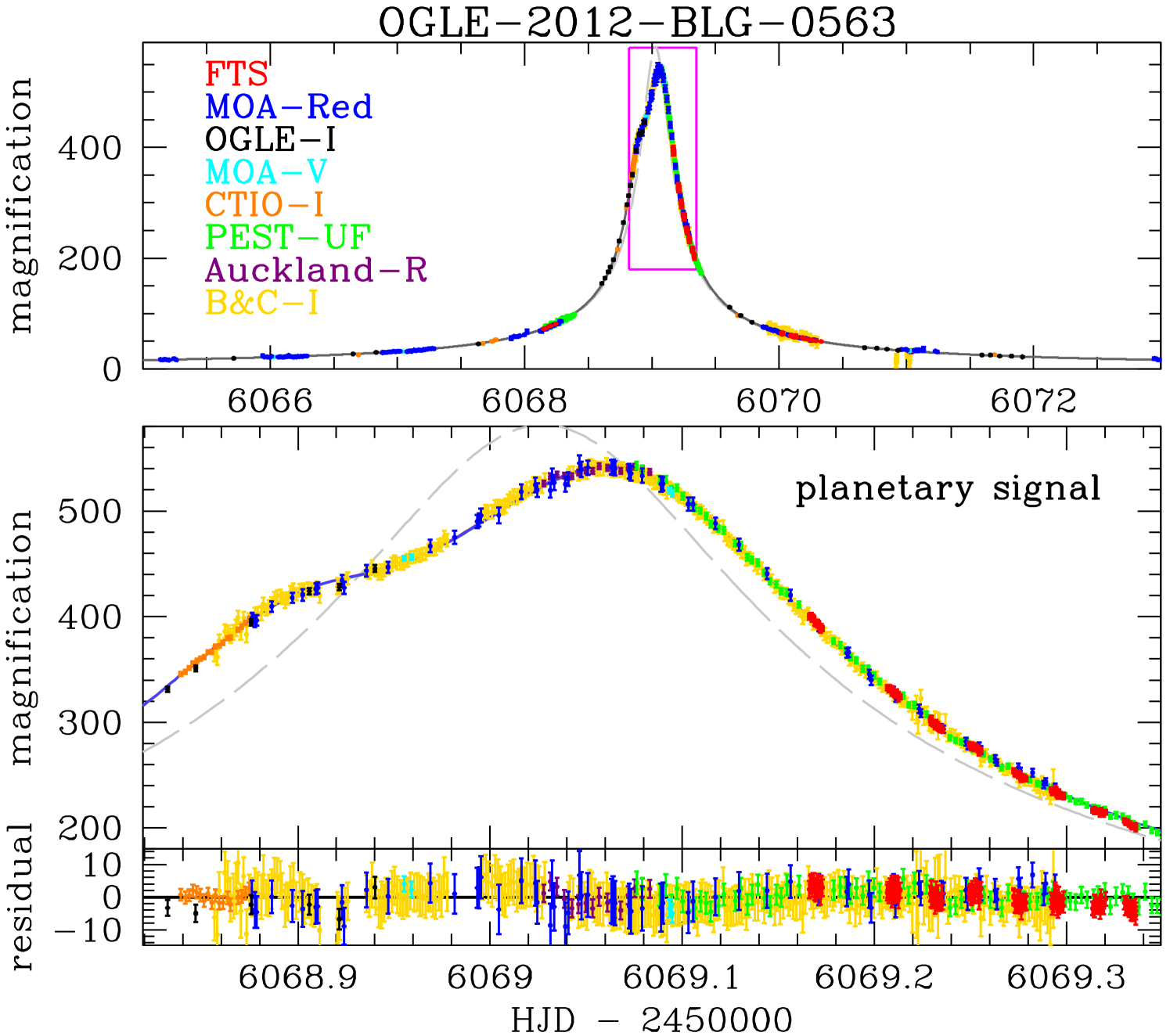
The microlensing event, OGLE-2012-BLG-0563, was independently discovered by the OGLE and MOA collaborations, as described in the Fukui et al. (2015) discovery paper (hereafter F15). Because it was predicted to reach high magnification, which implies a high sensitivity to planetary signals (Griest & Safizadeh, 1998; Rhie et al., 2000), the FUN and RoboNet groups began observations more that 20 hours prior to peak magnification. The MOA group also added observations with the 0.61m B&C telescope at MJUO in the -band filter at the Mt. John University Observatory (MJUO) in New Zealand on the night of peak magnification. The RoboNet group observed the event from the Faulkes Telescope South (FTS) 2.0m telescope at Siding Springs Observatory, the Faulkes Telescope North (FTN) in Hawaii, and the Liverpool Telescope (LT) in the Canary Islands. However, the FTN and LT data do not cover enough of the light curve to constrain the planetary models, so they are not included in any of our light curve modeling. The FUN group followed this event with the 1.3m SMARTS Telescope at CTIO in the , , and passbands, as a well as several amateur telescopes in New Zealand and Australia that were able to get good photometry at high magnification. We use -band data from the 0.4m Auckland Telescope and unfiltered data from the 0.3m PEST Telescope in Perth, Australia.
In addition to analyzing the light curve data, F15 also analyzed images of this target taken with the 8.2m Subaru telescope on Mauna Kea in Hawaii using adaptive optics on 2012 July 28 (HJD = 2456137.8), when the microlensing magnification had decreased to a factor of 1.3, according to our best fit model. These images had an angular resolution of , which is usually good enough to revolve the source from unrelated stars, but the lens-source separation at the time of these images was only , so the lens and source images could not be resolved into separate stellar images. Nevertheless, since the source brightness can usually be determined from the light curve model, it is possible to detect excess stellar flux at the position of the source and lens stars. If there is excess flux at the position of the source, there is a good chance that small or all of this excess flux is due to the lens star, which also hosts the planet. However, it is also possible that most of this excess flux could be due to a stellar companion to the lens or source star, or the chance superposition of a star that is unrelated to the microlensing event. These possibilities can be tested with follow-up images of the microlens system that measure the separation and relative proper motion of the source and candidate lens stars to determine if these are consistent with the microlensing model (e.g. Bennett et al., 2015; Batista et al., 2015) or not (Bhattacharya et al., 2017). Since the lens-source separation for OGLE-2012-BLG-0563 was far too small to be measured at the time of the Subaru observations, F15 consider the possibility that the excess flux is “contaminated” by flux from a star other than the lens star, such as a companion to the source or lens, or an unrelated star. They find that the implies host masses of , , and for contamination fractions of 0-10%, 10-30%, and 30-50%, respectively.
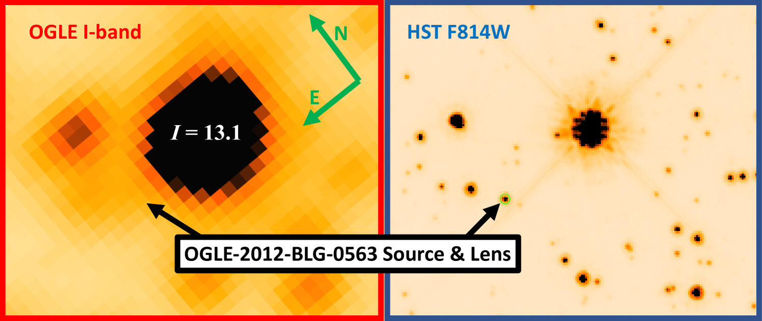
F15 also note that the light curve photometry for this microlensing event is challenging due to the presence of a bright star that is from the microlensing event. This location of the microlensed source star is shown in OGLE -band and Hubble -band (WFC3/UVIS/F814W) images in Figure 1. F15 state that “the photometry was carefully done to minimize systematics” due to this bright neighbor star. This star is saturated in most of the MOA images and in the best seeing OGLE images, and it is likely that systematic errors persist in the OGLE-2012-BLG-0653 light curve photometry, despite the best efforts of F15 to mitigate them.
One notable feature from the F15 analysis of this event is the relatively large angular Einstein radius, which was determined to be mas. This is the second largest value out of the 27 events with measurements in the S16 sample, after the two-planet event OGLE-2006-BLG-109 (Gaudi et al., 2008; Bennett et al., 2010). This large value contributes to the relatively small lens distance, kpc that they derive, with the minimal contamination fraction of 0-10%. (The inferred values are even smaller than this for larger assumed contamination fractions.) However, the most prescient section of (Penny et al., 2016) (section 6.2) pointed out that there was an excess of planets with claimed distances of kpc among the microlens planetary events that had been published at that time. There were six such events (OGLE-2006-BLG-109, MOA-2007-BLG-192, MOA-2010-BLG-328, OGLE-2012-BLG-0563, OGLE-2013-BLG-0341, and OGLE-2013-BLG-0723) whereas their simulations predicted only one, under the assumption that the planetary occurrence rate is independent of . In fact, many of these planetary events with claimed kpc have now been shown to be wrong. Event OGLE-2013-BLG-0723 was shown to have a very large microlensing parallax signal that was due to the use of an incorrect model (Han et al., 2016). The event is due to a stellar binary with no planetary signal. It was the attempt to fit the light curve to a binary star system with a planetary signal that drove the microlensing parallax parameter to an unusually large value. With the correct model, the inferred lens distance is kpc. Event MOA-2007-BLG-192 was also found to have an unusually large microlensing parallax value caused by a systematic error in the MOA data. Color dependent atmospheric refraction can generate systematic errors in difference imaging photometry because stars of different colors will have their positions shifted by different amounts, and this is especially significant in MOA data because of the unusually wide MOA-Red passband. This can induce seasonal systematic errors because color dependent centroid shifts are in different directions during the beginning and end of the Galactic bulge observing season. Detrending methods to remove these systematic errors (Bennett et al., 2012; Bond et al., 2017) have reduced both the microlensing parallax amplitude and the resulting lens system distance is kpc using detections of the host star in follow-up observations with both Hubble and Keck AO images (Terry et al., 2024).
The modeling of MOA-2010-BLG-328 is perhaps the most complicated. The discovery paper (Furusawa et al., 2013) presented two alternative models: one with a strong microlensing parallax signal and planetary orbital motion and one with a strong xallarap (source orbital motion) signal. In fact, the high angular resolution follow-up images indicate that all of these light curve features are needed, as well as the magnification of the source companion Vandorou et al. (in preparation). The final analysis for MOA-2010-BLG-328 reveals a source distance kpc, which is significantly larger than the distance of kpc, reported in the discovery paper (Furusawa et al., 2013).
In this paper, we show that the small value inferred by (Fukui et al., 2015) for the OGLE-2012-BLG-0563 lens system is due to a different type of systematic error, and the resulting lens system kpc. This leaves the two planet system OGLE-2006-BLG-109L and the planet in a binary system OGLE-2013-BLG-0341L (Gould et al., 2014) as the two remaining planetary events in the sample considered by Penny et al. (2016) at kpc. However, the OGLE-2013-BLG-0341 event also had a large microlensing parallax signal and a linear trend that seemed to be explained by the proper motion of a nearby star. However, OGLE data taken after publication failed to confirm this model to explain the linear trend, so it is unclear if the Gould et al. (2014) microlensing parallax signal is contaminated by a systematic error. Thus, of the six potentially suspect events with kpc from Penny et al. (2016), four have been shown to be wrong, one is uncertain, and only OGLE-2006-BLG-109L remains at kpc. This agrees with the conclusion of Penny et al. (2016) that “there is very little chance that the [OGLE-2006-BLG-109] distance estimate is significantly in error.”
We have applied the lessons from these other analyses to our analysis of this event. In particular, we have used the same detrending methods (Bennett et al., 2012; Bond et al., 2017) that were applied to the MOA-2007-BLG-192 follow-up imaging analysis (Terry et al., 2024) to this event. However, we found that the MOA data preferred a much fainter source and longer Einstein radius crossing time () than the OGLE data. This is not very surprising because very high magnification events are subject to a significant blending degeneracy (Alard, 1997; Di Stefano & Esin, 1995), because light curves with different and source magnitudes can only be distinguished by the low magnification parts of their light curves. The OGLE images have the benefits of a narrower passband, better seeing and a smaller angular pixel scale ( instead of ). The MOA pixels subtend an angle that is a factor of 2.2 larger than the OGLE pixels, but the typical seeing in MOA images is only about a factor of 1.5 larger than the typical OGLE seeing. This means that starlight in the OGLE images is spread over more pixels than in the MOA images, and the wider MOA-red passband also increases the number of photons detected per pixel in the MOA images, compared to OGLE. As a result, this bright neighbor star is saturated in a relatively small fraction of OGLE images, while it is saturated in most MOA images. Therefore, we have decided to exclude the MOA images taken more than five days before or after peak magnification at days in order to reduce the systematic photometry errors due to this bright neighbor star.
2.1 Keck Adaptive Optics Follow-up Imaging
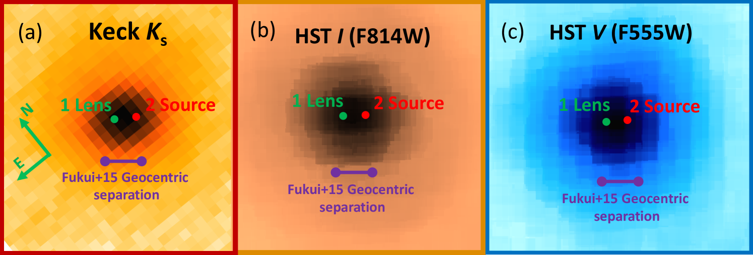
The analysis of Keck AO imaging of this target is presented in the Bhattacharya et al. (2024) companion paper. The analysis presented in this paper was based on 20 Keck NIRC2 images with a combined point-spread function (PSF) full-width half-max (FWHM) of mas. These images indicated two blended stars with a separation of mas and mas in the North and East directions, respectively. The separation vector has a length of mas, which is only 37% of the FWHM, so the apparent lens and source stars are only partially resolved in these Keck AO images, as illustrated in panels (a) and (d) of Figure 2.
Because of the strong overlap between the PSFs, the 2-star PSF models can trade flux between the two stars, resulting in a correlated uncertainty in their magnitudes. This analysis indicates that the combined brightness of the two stars is , where we use to refer to the NIRC2 and 2MASS bands in this paper. The two-star fit to the blended source and lens stars yields a magnitude difference of , where and refer to the stars toward the North-East and South-West, respectively. In section 3, we will show that the North-East star is the lens (and planetary host) star and South-West star is the source star. The inferred magnitudes of these stars are and , with a strong correlation between these magnitude uncertainties. F15 found , which is within of our value (if we combine the error bars), but their analysis is a bit more complicated because they had to correct for the microlensing magnification at the time of their Subaru observations. This analysis led to a source magnitude of , which involved a transformation from a light curve measurement in the band. Our removal of the low-magnification MOA data from microlensing light curve modeling of this event allowed the higher quality OGLE data to control the measured angular Einstein crossing time, , which implies a brighter source star. However, F15 find that the excess flux blended with the source star gives , which is within of the -band magnitudes of both of the stars that were identified in the 2-star fit to the OGLE-2012-BLG-0563 Keck images.
The results of our group’s analysis of the Keck images (Bhattacharya et al., 2024) differ somewhat from the predictions of the OGLE-2012-BLG-0563Lb discovery paper (Fukui et al., 2015). In particular, the discover paper predicted a relative lens-source proper motion of mas/yr. Since the Keck AO images were taken years after the peak of the OGLE-2012-BLG-0563 microlensing event, the predicted lens-source separation was mas, but a two star fit to the Keck AO blended stellar image at the location of the OGLE-2012-BLG-0563 yielded a separation of mas. So the discovery paper’s predicted separation from the light curve analysis is 65% larger than the measured separation from the Keck observations.
The fact that separation of the stars in our 2-star fit to the blended source-plus-lens image is only 37% of the PSF FWHM means that it would be very difficult to detect a third star located between the other two. Thus, it might be possible that the lens-source separation is consistent with the F15 prediction of mas if there was a third star located in between the lens and source stars.
In this case, however, there is an important difference between the coordinate systems used to determine the lens-source relative proper motions, . The light curve models can determine for events with finite source effects that determine the source radius crossing time, . The angular source radius, , is determined from the extinction-corrected magnitude and color of the source (e.g. Kervella et al., 2004; Boyajian et al., 2014; Adams et al., 2018), and then the amplitude of the lens-source relative proper motion is given by
| (1) |
The subscript, G, in equation 1 refers to the fact that this measurement or occurs in an inertial geocentric reference frame that moves with the Earth at the time of the peak of the microlensing event. In contrast, the two-dimensional relative proper motion vector measured with high angular resolution follow-up observations uses a heliocentric reference frame (plus a small contribution from geometric parallax that is almost always insignificant). In most cases, the difference between the heliocentric lens-source relative proper motion vector, , and the geocentric vector, is relatively small, but this is not the case for the “best fit” parameters for OGLE-2012-BLG-563 reported by F15.
The relationship between the geocentric and heliocentric lens-source proper motions is given by (Dong et al., 2009):
| (2) |
where is the projected velocity of the earth relative to the sun (perpendicular to the line-of-sight) at the time of peak magnification. This projected velocity is = (25.1075, 1.4462) km/sec = (5.2963, 0.3051) AU/yr at the peak of the for OGLE-2012-BLG-563 microlensing light curve. This is close to the Earth’s full orbital speed of km/sec because the event occurred near the middle of the Galactic bulge season. So, the Earth’s projected velocity term, , in equation 2 is larger than average, but the relative parallax, given by would be very much larger than average if we adopted the small lens distance, kpc reported by F15. When we insert the Earth’s projected velocity and the definition of into equation 2, we have
| (3) |
Using the F15 “best fit” values for the source distance, kpc and kpc, we can find the convert the measured to the geocentric coordinate system. However, the sign of the measured lens-source relative proper motion depends on which of the two stars is the source and which is the lens. Assuming the F15 and values, which we argue are incorrect in Section 4, we find that the vectors would be
|
|
(4) |
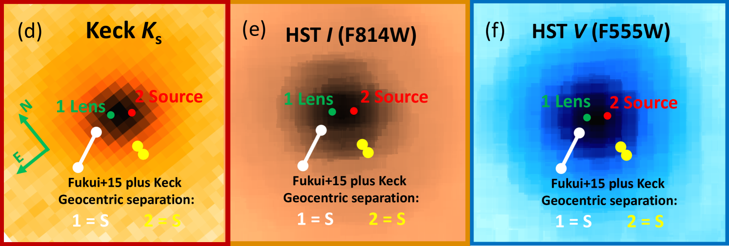
for these two choices of the source stars. The light curve models only provide the length of the vector, so these results would imply that the have lengths of mas/yr if star 1 is the source and mas/yr if star 2 is the source. These vectors are displayed as white and yellow lines in Figure 2 panels d, e and f. These give both the separation and the orientation of the two stars in the geocentric frame, but the Keck and Hubble images are in the heliocentric frame. Since the light curve only provides information on the magnitude of the vector, it is only the lengths of these vectors that should be compared with the F15 geocentric separation prediction shown in Figure 2 panels a, b and c. The F15 value of mas/yr, is only 1.3 smaller than the value for star 1 as the source, so this source identification would seem to be a better fit to the Keck data, as long as we assume that the F15 lens distance value of kpc is correct. However, the direction of the vector is identical to the direction of the vector and the length of the vector is proportional to the angular Einstein radius, , which is inversely proportional to the source radius crossing time, . Thus, constraints on also modify light curve parameters. As we discuss in our companion paper (Bhattacharya et al., 2024), our image-constrained modeling (Bennett et al., 2024) of this event raises some doubt that star 1 could be the source. When we apply the Keck constraints on the -band magnitude and measurement under the assumption that star 1 is the source, the fit rises by compared to the best light curve model without these constraints.
We should also note that the uncertainties in the host star mass and distance estimates reported by F15 are relatively large. Also, the mass-luminosity relation for a close binary host star system would imply that the lens system is more distant (Bennett et al., 2016), so the difference between and could be much smaller than implied by the “best fit” parameters reported by F15. So, the possibility that the lens-source separation measurement might be contaminated by a third star, as mentioned earlier in this section cannot be excluded on the basis of the Keck data.
3 Hubble Space Telescope Follow-up Observations and Analysis
| Passband | Star 1 mag | Star 2 mag | |||
|---|---|---|---|---|---|
| mas/yr | mas/yr | mas/yr | (lens) | (source) | |
| Keck | |||||
| HST F814W () | |||||
| HST F555W () | |||||
| weighted mean |
The Heliocentric relative proper motion and magnitude measurements for stars 1 and 2. The relative proper motion refers to the motion of star 1 minus star 2.
On 2018 May 26, we obtained a single orbit of Hubble observations from program GO-15455, using the WFC3/UVIS camera. This was 6.009191 years after the peak of the event, and just about 45 hours after the Keck observations that were taken 6.004040 years after the peak of the even. We obtained sec. dithered exposures with the F814W filter and sec. dithered exposures with the F555W filter using the UVIS2-C1K1C-SUB aperture to minimize CTE One image in each of these passbands was taken in the .UVIS2-2K2C-SUB aperture, but these were not used in the analysis. (The Hubble data used in this paper can be found in MAST: http://dx.doi.org/10.17909/wd7f-vv60 (catalog 10.17909/wd7f-vv60).) The analysis was done with a modified version of the codes based on an early version of hst1pass (Anderson, 2022) used by Bennett et al. (2015) and Bhattacharya et al. (2018). It differs from hst1pass in that is has specialized routines to accurately measure the photometry and astrometry of partially resolved stars, due coordinate transformations to Keck images and to calibrate photometry to the OGLE-III database (Szymański et al., 2011). Like hst1pass, our Hubble analysis code analyze the data from the original images without any resampling in order to avoid the loss of resolution that the combination of dithered, undersampled images would provide.
The coordinate transformation between the Keck and Hubble images was done with 16 stars brighter than , yielding the transformation
|
|
(5) |
from Keck to Hubble WFC3/UVIS pixels. The RMS scatter for this relation is mas and mas, since the WFC3/UVIS pixels subtend 40 mas. This separation is small because the time interval between the images is days, so the offset due to stellar proper motion is negligible.
The Hubble photometry was calibrated to the OGLE-III catalog (Szymański et al., 2011) using 7 relatively bright OGLE-III stars stars in the band and 5 bright stars in the band. These stars were selected because they had no nearby neighbors that were close enough to contaminate the OGLE photometry. The RMS scatter of these stars to the best fit photometry zero-point was 0.0265 magnitude in the -band and 0.0285 magnitudes in the -band. We assume a calibration uncertainty of 0.04 magnitudes that is added in quadrature to the uncertainties in the instrumental magnitudes to get the results reported in Table 1.
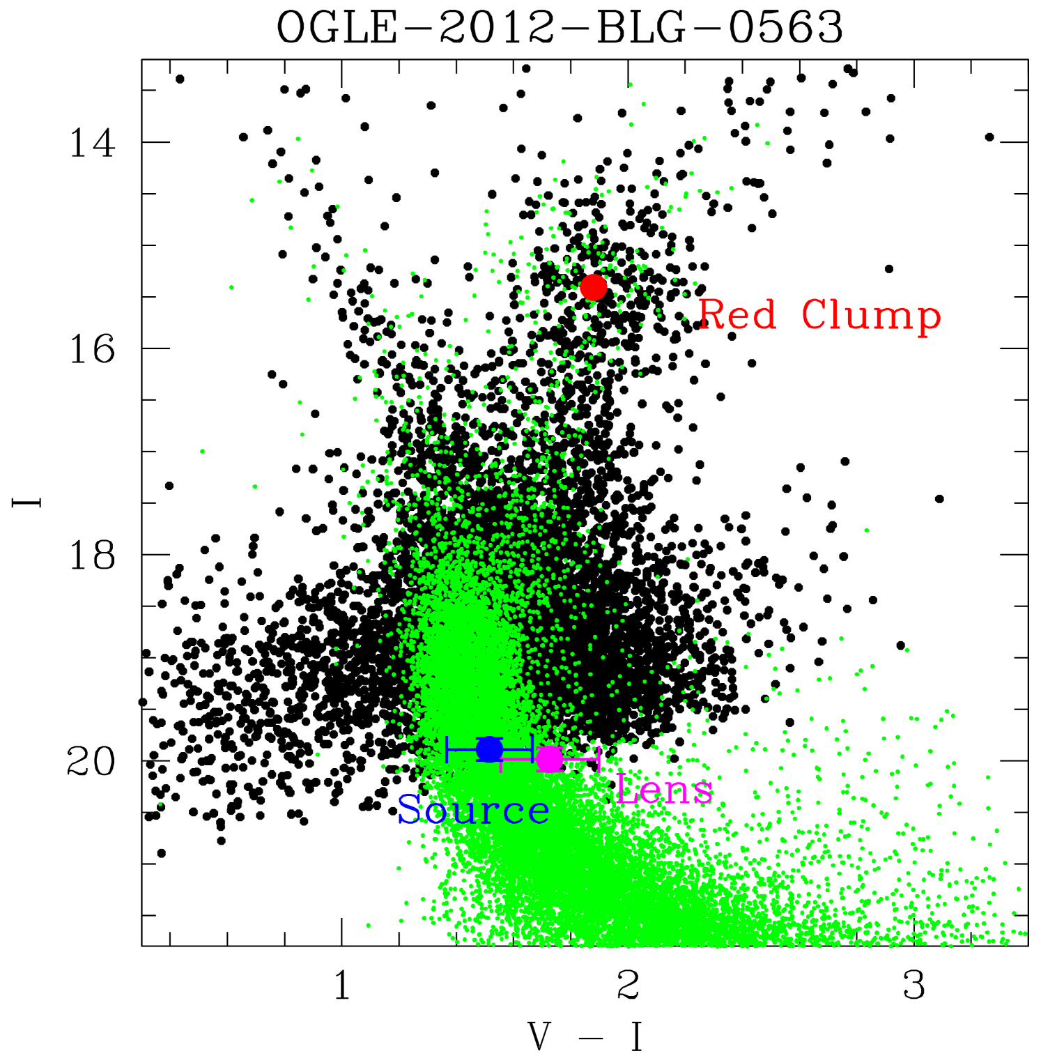
The locations of the stars 1 and 2 are shown as magenta and blue dots on the OGLE-III color magnitude diagram in Figure 3, where they are labeled as the lens and source stars, respectively based on the arguments given below. The green points in Figure 3 are from the Holtzman et al. (1998) Baade’s Window color magnitude diagram, converted to the same extinction and Galactic bar distance as the OGLE-2012-BLG-0563S source star. Star 1 is located on the red edge of the bulge main sequence, as we would expect for an intrinsically fainter and slightly redder lens star in the foreground of the bulge
Following Bennett et al. (2014), we determine the and band extinction from the stars of the OGLE-2012-BLG-0563S source by measuring the centroid of the red clump giant stars. We find and , Following Nataf et al. (2013), we use an intrinsic red clump star magnitude and color of and . This yields extinction values of and , implying a color excess of .
The coordinate transformation in equation 5 enables us to put the relative proper motion measurements () from Keck and Hubble on the same Heliocentric coordinate system, as shown in Table 1, which also indicates the calibrated magnitudes for stars 1 and 2 in all three passbands (, , and ). The colors of the two stars are and . We use the OGLE-III photometry catalog (Szymański et al., 2011) and the Nataf et al. (2013) red clump star color magnitude centroid values at the Galactic longitude of this event to find extinction values of and . These are similar to the values of and reported by F15. We find a -band extinction of , from the Surot et al. (2020) value of the color excess at the OGLE-2012-BLG-0563 location using the Nishiyama et al. (2006) infrared extinction law. So, the extinction corrected magnitude and colors for star 2 are , and , which is consistent with a G-dwarf in the bulge, as inferred by F15. For star 1, we find , and , assuming the same extinction as the red clump centroid.
We performed a preliminary light curve analysis using all the light curve data from F15, except the MOA data was reduced by an improved MOA photometry code (Bond et al., 2001, 2017) for both the custom MOA-red passband and the MOA-V passband. These were also calibrated to the OGLE-III catalog (Szymański et al., 2011) . These results indicated preliminary calibrated source star magnitudes of and , which are consistent with the identification of star 1 as the source.
These measurements do not match the conclusions of F15, who reported a host star mass of , at a distance of kpc. A host star of would have a color of with the same extinction as the source, or with only half the extinction of the source, which is still 1.65 magnitudes redder than star 1. Even a star at the 2 mass upper limit or , would have , which is redder than star 1, assuming half the extinction of the source star. Thus, it seems unlikely that our high angular resolution follow-up observations will confirm the F15 analysis.
| with FTS, B&C data | no FTS, B&C data | |||
|---|---|---|---|---|
| parameter | unconstrained | only | constrainted | constrainted |
| (days) | 62.058 | 62.157 | 63.979 | 63.768 |
| () | 6069.0290 | 6069.0291 | 6069.0275 | 6069.0281 |
| -0.0017541 | - 0.0017550 | -0.0017192 | -0.0017281 | |
| 0.40159 | 0.40559 | 0.41513 | 0.42452 | |
| (rad) | 0.49856 | 0.49769 | 0.49397 | 0.49231 |
| 1.4891 | 1.4604 | 1.3866 | 1.3088 | |
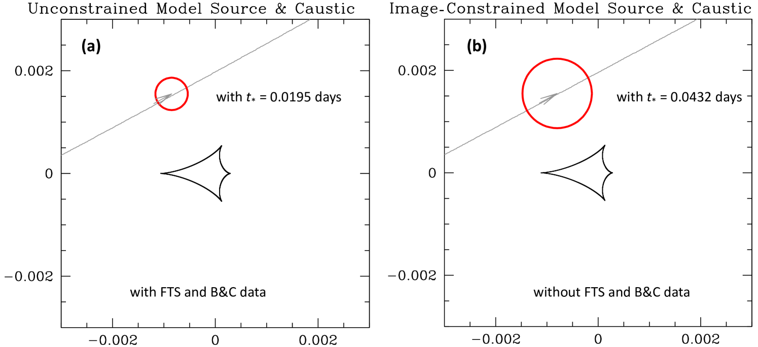
| (days) | 0.01951 | 0.02488 | 0.04004 | 0.04319 |
| 0.59927 | 0.60754 | 0.05361 | 0.05821 | |
| 0.11011 | 0.11019 | 0.08207 | 0.07955 | |
| (kpc) | - | 8.0306 | 8.8438 | 8.4531 |
| FTS | 185.52 | 187.55 | 213.516 | - |
| B&C | 528.29 | 529.84 | 542.155 | - |
| OGLE- | 670.04 | 667.80 | 662.199 | 660.094 |
| MOA-Red | 164.804 | 164.231 | 165.390 | 159.305 |
| light curve | 2064.65 | 2066.13 | 2100.75 | 1344.10 |
| dof | ||||
| (no FTS,B&C) | 1350.84 | 1348.74 | 1345.07 | 1344.10 |
| dof(no FTS,B&C) | ||||
| (kpc) | - | 1.154 | 5.586 | 5.424 |
| - | 0.239 | 0.843 | 0.835 | |
| (mas) | 1.532 | 1.201 | 0.673 | 0.670 |
The values use an inertial geocentric coordinate system that moves with the Earth at . The image constraints increase source radius crossing time, and and decrease the implied angular Einstein radius, (both highlighted in bold-face) by a factor of .
In order to investigate this, we modeled this event with the image-constrained modeling version of the eesunhong111https://github.com/golmschenk/eesunhong light curve modeling code, described in detail in Bennett (2010); Bennett et al. (2024). This code includes Gaussian constraints for seven of the measurements listed in Table 1. These include the weighted mean values of the North and East components of , using both the Keck and Hubble data, the , , and host star magnitudes, and the and source star magnitudes. (Because we have no light curve measurements in the band, we impose no constraints on the source magnitude.) Also, because the separation of the lens and source stars is % of the FWHM of the Keck images and only 62% of a Hubble WFC3/UVIS pixel, the images of the lens and source stars have significant overlap, and this results in a significant correlation between their magnitude measurements. A fainter magnitude for one star can be compensated by a brighter magnitude for the other. As a result, the magnitude of the combined lens plus source stars can be determined more precisely than the individual magnitudes. Therefore, we impose two additional constraints on the combined lens and source magnitudes, and .
These constraints change the model results quite dramatically,, as Table 2 indicates. The second column of this table gives the fit results with no constraints, and the third column gives the with only the constraint on the -band magnitude of the lens, , which yield essentially the same same conclusions as the F15 paper. The fifth column gives the best fit model after removing two data sets that have apparent systematic errors that we discuss in the next section. However, the addition of the constraints on , and the lens and source magnitudes increased the best fit source radius crossing time, , by a factor of , over the best fit unconstrained model. This has a direct effect on the inferred angular Einstein radius, , which decreases by a factor of .
4 Systematic Errors in Light Curve Photometry
The existence of these systematic errors was foreshadowed by the inset plot in Figure 1 of F15 which shows the central caustic, the source trajectory, and the source size for their best fit model. Figure 4 shows a comparison of the central caustic and the source star trajectory and radius, for the best fit model with no image constraints, including the FTS and B&C data (a) and our final result with the high angular resolution image constraints (b), which excludes the FTS and B&C data. While the central caustic in panels (a) and (b) of Figure 4 look nearly identical, the source radius in panel (b), with the the constrained fit, is twice the size of the source radius in panel (a). This is due to the larger source radius crossing time for the image-constrained fit, as indicated in the second and fifth columns of Table 2. For the unconstrained fit parameters illustrated in Figure 4(a), the limb of the source star is always at least 3.7 source star radii from the central central caustic. This is surprising because finite source effects typically are not detectable, unless the limb of the source star passes within source radii of the caustic, which is the minimum separation between the source star limb can central caustic for the image-constrained fit, illustrated in Figure 4(b).
Table 2 also lists the values for four of the data sets used in the light curve modeling in order to show which data sets are driving the unconstrained fit towards very small source radius crossing times. For most microlensing events, it is the OGLE data that suffers the least degradation from systematic errors, due to the excellent seeing at the OGLE observing site at the Las Campanas Observatory, and highly optimized photometry code (Udalski et al., 2015a), and we see that the of the OGLE- photometry is improved by the image constrained models. However, the FTS increases by and the B&C is increased by when the image constraints are applied to the modeling.
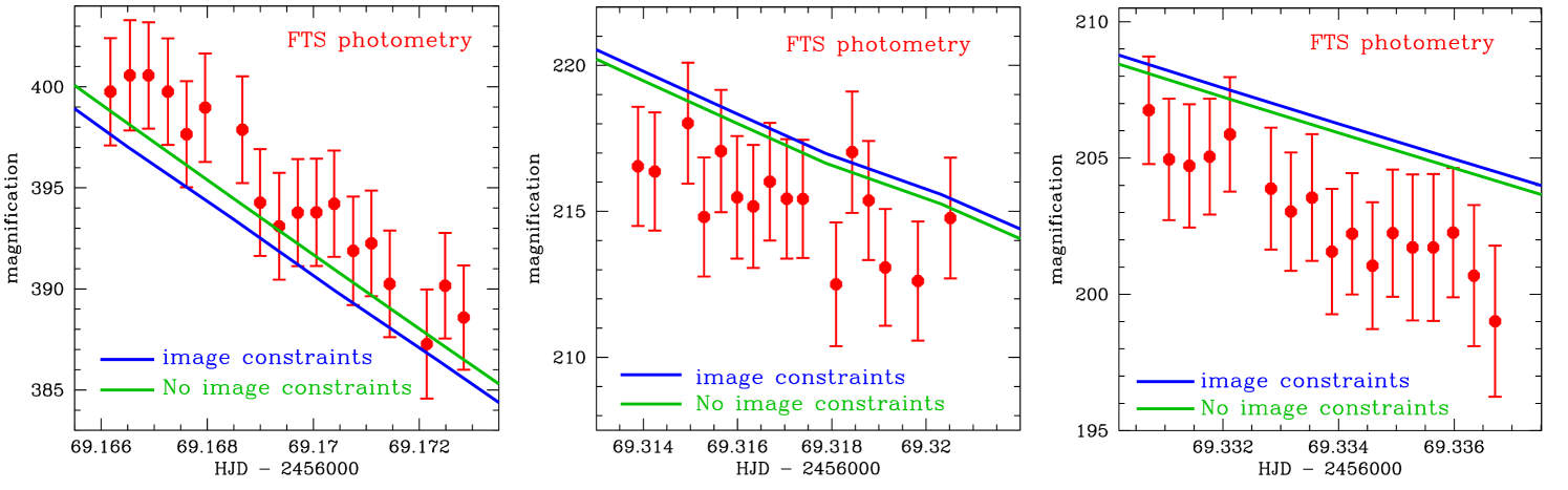
In order to investigate this discrepancy between the high angular resolution imaging results and photometry from FTS and B&C data, we take a closer look at the best image-constrained model, including all the data considered in this paper, which is displayed in Figure 5. The FTS data is displayed in red, and it consists of a series of continuous observations for periods of about 10 minutes at about a three hour interval. The residual plot at the bottom of Figure 5 shows that the FTS data gradually drifts from above the model light curve to below the light curve over the time span of the FTS observations on the night of the light curve peak.
Figure 6 shows close-ups of the first and last two (which are fourth and fifth) of these FTS observing periods, with the best fit model with and without the image constraints shown in blue and green, respectively. Note that neither model is a good fit to the FTS data, and the difference between the blue and green curves is much smaller than the difference between the data and either curve. Thus, it seems likely that the offset between the data and both models is due to a systematic error in the FTS data. As mentioned in section 2 and illustrated in Figure 1, the photometry of this star is prone to systematic errors due to the proximity of a very bright star. We also note that it is more difficult to identify systematic errors in photometry from telescopes that are used to follow-up potential planetary microlensing events than it is for microlensing survey telescopes, like the MOA and OGLE telescopes. This is because the survey telescopes include a large number of observations in varying observing conditions without significant microlensing magnification. These can be used to identify systematic errors and possibly remove them with detrending methods (Bennett et al., 2012; Bond et al., 2017). In contrast, the data from follow-up telescopes often only include data with significant microlensing magnification, and so it can be difficult to differentiate between systematic errors and higher order microlensing effects. Finally, these follow-up telescopes often focus a much larger fraction of their observing time on candidate microlensing events, so they may have many more observations than the survey telescopes. This can allow their systematic errors to dominate some light curve model features over the survey telescopes (and OGLE, in particular), which are generally less prone to systematic photometry errors.
| parameter | MCMC averages | ||||
|---|---|---|---|---|---|
| (days) | 63.768 | 63.818 | 63.773 | 64.166 | |
| () | 6069.0281 | 6068.8862 | 6069.0280 | 6068.8812 | |
| -0.0017281 | -0.0005312 | 0.0017294 | 0.0004917 | ||
| () | |||||
| 0.42452 | 2.36105 | 0.42416 | 2.38039 | ||
| () | |||||
| (rad) | 0.49231 | 0.49249 | -0.49171 | -0.49185 | |
| () | |||||
| 1.3088 | 1.3070 | 1.3098 | 1.3273 | ||
| (days) | 0.04319 | 0.04312 | 0.04305 | 0.04255 | |
| 0.05821 | 0.05788 | 0.05814 | 0.05896 | ||
| 0.07955 | 0.08079 | 0.07971 | 0.08067 | ||
| (kpc) | 8.4531 | 8.2873 | 8.4462 | 8.3923 | |
| (mas) | 0.6704 | 0.6698 | 0.6707 | 0.6752 | |
| fit | 1347.37 | 1347.97 | 1350.25 | 1350.63 | |
| dof | |||||
The values are based on the inertial geocentric coordinate system that moves with
the Earth at .
Also, the time period covered by the FTS data is also covered by a number of other data sets including MOA and the Perth Exoplanet Survey Telescope (PEST), and these data sets do not favor the deviations from the light curve models seen by FTS. Therefore, we remove the FTS data from our final light curve modeling. The B&C data also had a increase when the image constraints are added to the modeling, but the increase is smaller than the increase from the FTS data, while the number of B&C observations are larger. So, it is difficult to generate a figure similar to Figure 6 that offers a clear indication of systematic errors. However, B&C has also proved to be problematic for some previously analyzed events, so we drop this data as well. As columns 4 and 5 of Table 2 show, the removal of the FTS and B&C data has only a small effect on the best fit model parameters. We remove it because it would be likely to induce unreasonably small error bars on the inferred parameters of the planetary microlens system.
5 Lens Properties
Our final modeling of this event excludes the FTS and B&C data, yielding the best fit model parameters indicated in the fifth column of Table 2. We use the same image-constrained modeling method presented in Bennett et al. (2024). We used Gaussian constraints listed in Table 1 for the weighted mean and values and the lens and source magnitudes, except that there is no -band light curve data to be constrained with the source -band measurement from Keck. We also constrain the combined lens and source magnitudes to be and , as mentioned in Section 3. In addition to these nine constraints, we also constrain the source distance, using a Galactic model prior from Koshimoto et al. (2021a).
The model source magnitude values for these constraints come from our calibrations of the light curve photometry, but the lens magnitudes come from the empirical mass-luminosity relations presented in Bennett et al. (2018b, 2020). In addition to these mass-luminosity relations, we must also account for the dust extinction as a function of lens distance. At Galactic coordinates of and , the extinction towards the lens system can be almost as large as the extinction to the source star, unless the lens system is unusually close to the observer, as was the case for the F15 analysis. We assume a dust scale height of kpc (Drimmel & Spergel, 2001), so that the extinction in the foreground of the lens is given by
| (6) |
where the index refers to the passband: , , or .
| parameter | units | values & RMS | 2- range |
|---|---|---|---|
| Angular Einstein Radius, | mas | 0.611–0.681 | |
| Geocentric lens-source relative proper motion, | mas/yr | 3.619–3.770 | |
| Host star mass, | 0.736–0.866 | ||
| Planet mass, | 0.952–1.300 | ||
| Host star - Planet 2D separation, | AU | 1.24–9.90 | |
| Host star - Planet 2D sep. (close), | AU | 1.20–1.81 | |
| Host star - Planet 2D sep. (wide), | AU | 6.75–10.18 | |
| Host star - Planet 3D separation, | AU | 1.33–28.06 | |
| Lens distance, | kpc | 4.45–6.64 | |
| Source distance, | kpc | 6.41–10.88 |
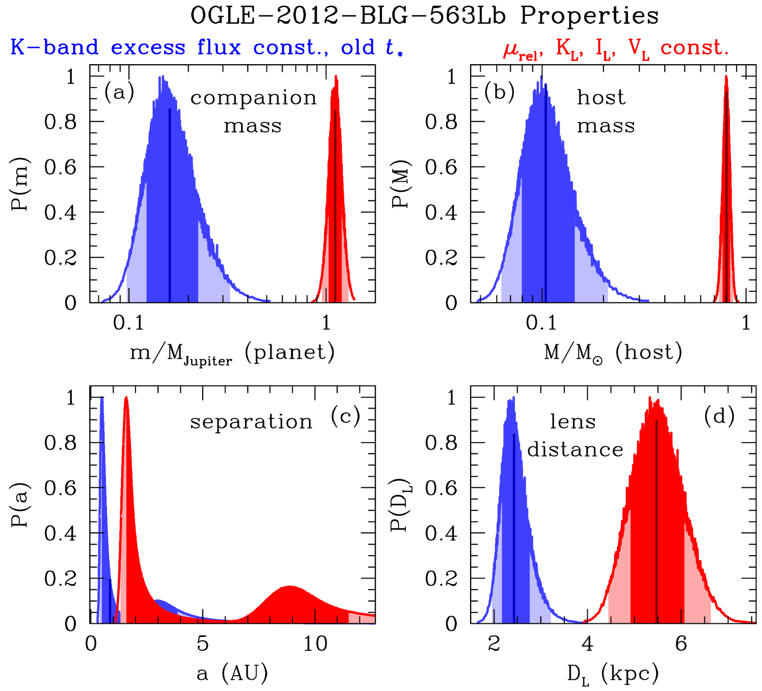
High magnification events like OGLE-2012-BLG-0563 are subject to the close-wide degeneracy (Dominik, 1999) due to the fact the that the model parameter transformation leaves the characteristics of the central caustic almost unchanged. A more general version of this degeneracy has been described by Zhang et al. (2022). Galactic bulge microlensing events observed toward the Galactic bulge with microlensing parallax signals are also subject to the ecliptic degeneracy (Poindexter et al., 2005), which is exact for events in the ecliptic plane. This degeneracy involves replacing a binary lens system with its mirror image, and it is the orbital motion of the Earth, which is detected via the microlensing parallax effect, that breaks the mirror symmetry. This ecliptic degeneracy results in a sign change for the for the and parameters. These two degeneracies lead to the four degenerate models. The parameters for the best fit models in each of these degenerate categories are given in Table 3. This table also shows the results of our Markov Chain Monte Carlo calculations over all the degenerate model. The parameters are quite similar for all four degenerate, except for the parameters directly affected by the degeneracies: , , and . The parameters and are not generally considered to be physically interesting because these just depend on the detailed alignment between the lens and source and the orientation of the lens system (which is thought to be random). For events with , the degeneracy has little effect on the inferred physical parameters (e.g. Batista et al., 2015; Bennett et al., 2016, 2024; Bhattacharya et al., 2018), because the uncertainty due to the unobserved line-of-sight separation is larger than the difference between the close and wide solutions. However, for OGLE-2012-BLG-0563, the close and wide solutions have projected separations that differ by a factor of , so the orbital separations predicted by the close and wide solutions have very little overlap, as shown by the red curve in Figure 7(c) and the host star and planet 2D separation values listed in Table 4. This indicates that the host star is a K dwarf with a mass of , at a distance of kpc, orbited by a planet of mass . The separation of the planet from its host star is less certain, due to the close-wide light curve model degeneracy. The 2-dimensional planet-host star separation is for the close solution and for the wide solution, with a 2- range of 1.24–9.90 AU, when both solutions are considered. If we assume a random orientation of the planetary lens system, we find a 2- range of 1.33–28.06 AU, for the 3-dimensional separation.
Figure 7 also compares the planetary system properties found by our analysis to the results of a similar analysis using only the constraints considered in the F15 paper. However, this comparison analysis using the full data set, including the FTS and B&C data with only the magnitude constraint yields a slightly different result that the one reported by F15. Figure 8 of F15 indicates a double-peaked host mass and distance distribution with a sharp peak at , kpc and a broader peak at , kpc. Part of the reason for this difference is illustrated by Figure 7 of F15, which shows that the mass-distance relations from the angular Einstein radius, and the lens band magnitude, , are nearly parallel and have a significant overlap for kpc. The F15 analysis also assumes that the interstellar extinction is uniformly distributed along the line-of-sight to the source, which ignores measures that show the dust scale height in the Galactic disk is much lower than the scale height of the stars (Drimmel & Spergel, 2001) as represented by equation 6. Thus, F15 underestimate the extinction toward possible host stars at smaller distances (i.e. kpc). A more realistic extinction estimate would increase the mass-distance relation in Figure 7 of F15. Other differences between our analysis and that of F15 are that we have used re-reduced photometry using an improved method (Bond et al., 2017) and we have used an empirical mass-luminosity relation.
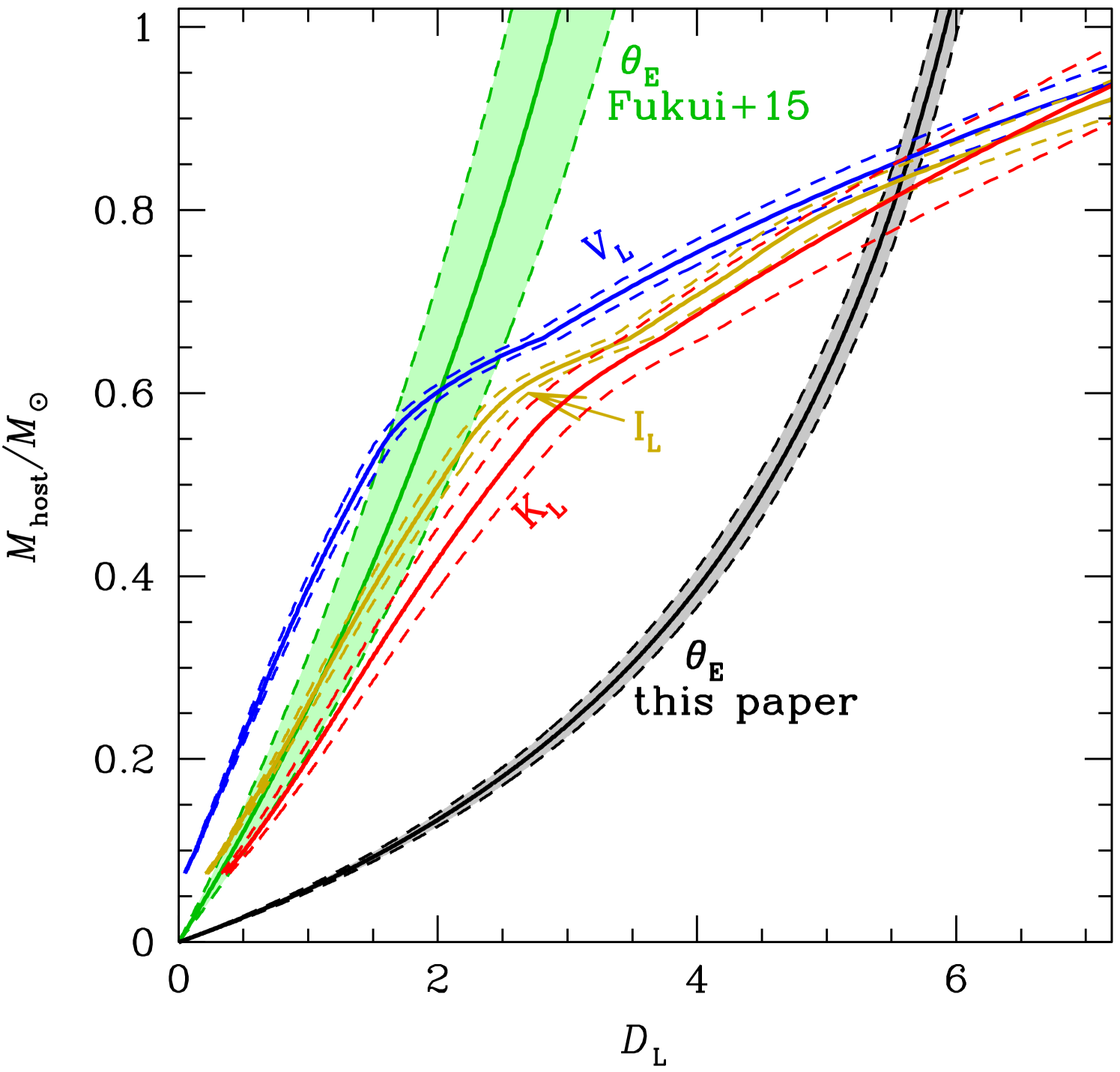
It may seem odd that a reduction in the inferred angular Einstein radius would lead to a significant increase in the implied mass of the lens system, because the mass-distance relation,
| (7) |
implies that the increases quadratically with . Of course, the answer is that the lens mass depends on both its distance, , and . Figure 8 displays a comparison of the effects of the determinations by F15 and our analysis with the lens magnitude constraints in the , , and passbands. The band lens magnitude constraint only intersects with the F15 curve at very small distances and very low host masses, but the and and especially the band curves intersect with the F15 curve at larger distances and masses. This is an indication of the systematic photometry error that led to the overestimate of the F15 value. Note that Figure 8 is a simplified presentation of the results. It includes the uncertainties on the measured host star magnitudes, and the average error bars for the , but the results presented in Figure 7 and Table 4 also include the effects of correlations with the other event model parameters from the MCMC analysis.
6 Conclusions
Our analysis of the 2018 Hubble images for planetary microlensing event OGLE-2012-BLG-0563 finds a substantially larger mass and distance for the planetary system with host star and planet masses of and , respectively. They are located at a distance of towards the Galactic bulge, with a projected star-planet separation of AU or AU, depending on whether the degenerate close or wide model is correct. Our light curve analysis used the image-constrained modeling version (Bennett et al., 2024) of the eesunhong (Bennett & Rhie, 1996; Bennett, 2010) light curve modeling code. This modeling revealed a discrepancy between the source radius crossing time, , favored by some of the light curve data from microlensing follow-up observations and the measured lens-source relative proper motion, , measured independently by Hubble images in the and bands, as well as Keck adaptive optics images in the band (Bhattacharya et al., 2024). This suspect ground-based photometry from the Faulkes South Telescope (FTS) to a lesser extent the MJUO B&C Telescope was investigated and found to be due to a minor improvement, that only slightly reduced a discrepancy from every model light curve, including the light curve with the small favored by this data. Also, the values for the data sets that are historically the most reliable, such as OGLE, were improved when the high angular resolution imaging constraints were added to the modeling.
The analysis of this event also indicates the importance of redundant methods for determining that mass and distances for planetary systems found by microlensing. In this case, have mass-distance relations from observations in three passbands, redundant determinations of from light curve measurements of the source radius crossing time, , and measurements of the lens-source relative proper motion, , from the high angular resolution follow-up observations. These values also provide a mass-distance relation, as indicated in Figure 8 and equation 7. Also, the image-constrained modeling enforces consistency between the implied lens mass from its magnitudes, the value, and the microlensing parallax light curve parameters, . These redundant constraints on the physical parameters of the planetary microlensing system allowed the systematic errors in the light curve photometry to be quickly identified and corrected.
We anticipate that this image-constrained modeling method will be very useful for analyzing the microlens planetary systems discovered by the exoplanet microlensing survey of the Nancy Grace Roman Space Telescope (Bennett et al., 2010a, 2018a; Spergel et al., 2015; Penny et al., 2019). This survey, known as the Roman Galactic Exoplanet Survey (RGES), will use the same methods to determine the masses of and distance to planetary microlensing systems as we have done with high angular resolution follow-up data from Keck and Hubble, except that the high angular resolution RGES images will be employed to determine the image constraints. RGES photometry will generally not be affected by the same types of systematic errors that we have discovered in the ground-based photometry used for the Suzuki et al. (2016) statistical sample of planetary microlensing events. However, the Roman Space Telescope employs a new generation of infrared detectors. While these detectors have improved sensitivity over previous generations of infrared detector (Mosby et al., 2020; Zandian et al., 2023), their improved sensitivity is likely to reveal subtle systematic errors that were not apparent in data from previous generations of detectors. We expect that the image-constrained light curve modeling method will enable any such systematic errors to be efficiently identified.
References
- Adams et al. (2018) Adams, A. D., Boyajian, T. S., & von Braun, K. 2018, MNRAS, 473, 3608. doi:10.1093/mnras/stx2367
- Alard (1997) Alard, C. 1997, A&A, 321, 424
- Anderson (2022) Anderson, J. 2022, Instrument Science Report WFC3 2022-5, 55 pages
- Bachelet et al. (2012) Bachelet, E., Fouqué, P., Han, C., et al. 2012, A&A, 547, A55
- Batista et al. (2015) Batista, V., Beaulieu, J.-P., Bennett, D.P., et al. 2015, ApJ, 808, 170 5
- Beaulieu (2018) Beaulieu, J.-P. 2018, Universe, 4, 61. doi:10.3390/universe4040061
- Bennett (2010) Bennett, D.P. 2010, ApJ, 716, 1408
- Bennett et al. (2018a) Bennett, D. P., Akeson, R., Anderson, J., et al. 2018a, (arXiv:1803.08564)
- Bennett et al. (2010a) Bennett, D. P., Anderson, J., Beaulieu, J.-P., et al. 2010a, RFI Response for the Astro2010 decadal survey, arXiv:1012.4486
- Bennett et al. (2007) Bennett, D.P., Anderson, J., & Gaudi, B.S. 2007, ApJ, 660, 781
- Bennett et al. (2014) Bennett, D. P., Batista, V., Bond, I. A., et al. 2014, ApJ, 785, 155
- Bennett et al. (2015) Bennett, D. P., Bhattacharya, A., Anderson, J., et al. 2015, ApJ, 808, 169
- Bennett et al. (2020) Bennett, D. P., Bhattacharya, A., Beaulieu, J.-P., et al. 2020, AJ, 159, 68. doi:10.3847/1538-3881/ab6212
- Bennett et al. (2024) Bennett, D. P., Bhattacharya, A., Beaulieu, J.-P., et al. 2024, AJ, 168, 15. doi:10.3847/1538-3881/ad4880
- Bennett et al. (2008) Bennett, D. P., Bond, I. A., Udalski, A., et al. 2008, ApJ, 684, 663
- Bennett & Khavinson (2014) Bennett, D. P. & Khavinson, D. 2014, Physics Today, 67, 64. doi:10.1063/PT.3.2318
- Bennett & Rhie (1996) Bennett, D.P. & Rhie, S.H. 1996, ApJ, 472, 660
- Bennett & Rhie (2002) Bennett, D.P. & Rhie, S.H. 2002, ApJ, 574, 985
- Bennett et al. (2010) Bennett, D. P., Rhie, S. H., Nikolaev, S., et al. 2010b, ApJ, 713, 837
- Bennett et al. (2016) Bennett, D.P., Rhie, S.H., Udalski, A., et al. 2016, AJ, 152, 125
- Bennett et al. (2012) Bennett, D. P., Sumi, T., Bond, I. A., et al. 2012, ApJ, 757, 119
- Bennett et al. (2018b) Bennett, D. P., Udalski, A., Bond, I. A., et al. 2018b, AJ, 156, 113
- Bennett et al. (2018a) Bennett, D. P., Udalski, A., Han, C., et al. 2018a, AJ, 155, 141
- Bhattacharya et al. (2017) Bhattacharya, A., Bennett, D. P., Anderson, J., et al. 2017, AJ, 154, 59
- Bhattacharya et al. (2018) Bhattacharya, A., Beaulieu, J.-P., Bennett, D. P., et al. 2018, AJ, 156, 289
- Bhattacharya et al. (2021) Bhattacharya, A., Bennett, D. P., Beaulieu J. P., et al. 2021, AJ, 162, 60
- Bhattacharya et al. (2024) Bhattacharya, A., et al. 2021, AJ, submitted
- Blackman et al. (2021) Blackman, J. W., Beaulieu, J. P., Bennett, D. P., et al. 2021, Nature, 598, 272. doi:10.1038/s41586-021-03869-6
- Bond et al. (2001) Bond, I. A., Abe, F., Dodd, R. J., et al. 2001, MNRAS, 327, 868
- Bond et al. (2017) Bond, I. A., Bennett, D. P., Sumi, T., et al. 2017, MNRAS, 469, 2434. doi:10.1093/mnras/stx1049
- Boyajian et al. (2014) Boyajian, T.S., van Belle, G., & von Braun, K., 2014, AJ, 147, 47
- Di Stefano & Esin (1995) Di Stefano, R., & Esin, A. A. 1995, ApJ, 448, L1
- Dominik (1999) Dominik, M. 1999, A&A, 349, 108. doi:10.48550/arXiv.astro-ph/9903014
- Dong et al. (2009) Dong, S., Gould, A., Udalski, A., et al. 2009b, ApJ, 695, 970
- Drimmel & Spergel (2001) Drimmel, R., & Spergel, D. N. 2001, ApJ, 556, 181
- Fukui et al. (2015) Fukui, A., Gould, A., Sumi, T., et al. 2015, ApJ, 809, 74
- Furusawa et al. (2013) Furusawa, K., Udalski, A., Sumi, T., et al. 2013, ApJ, 779, 91
- Gaudi et al. (2008) Gaudi, B. S., Bennett, D. P., Udalski, A., et al. 2008, Science, 319, 927
- Gould (2014) Gould, A. 2014, J. Kor. Ast. Soc., 47, 215
- Gould et al. (2014) Gould, A., Udalski, A., Shin, I.-G., et al. 2014, Science, 345, 46
- Griest & Safizadeh (1998) Griest, K., & Safizadeh, N. 1998, ApJ, 500, 37
- Han et al. (2016) Han, C., Bennett, D. P., Udalski, A., et al. 2016, ApJ, 825, 8. doi:10.3847/0004-637X/825/1/8
- Holtzman et al. (1998) Holtzman, J. A., Watson, A. M., Baum, W. A., et al. 1998, AJ, 115, 1946
- Janczak et al. (2010) Janczak, J., Fukui, A., Dong, S., et al. 2010, ApJ, 711, 731
- Kervella et al. (2004) Kervella, P., Thévenin, F., Di Folco, E., & Ségransan, D. 2004, A&A, 426, 297
- Kim et al. (2021) Kim, H.-W., Hwang, K.-H., Gould, A., et al. 2021, AJ, 162, 15. doi:10.3847/1538-3881/abfc4a
- Koshimoto et al. (2021a) Koshimoto, N., Baba, J., & Bennett, D. P. 2021a, ApJ, 917, 78. doi:10.3847/1538-4357/ac07a8
- Koshimoto et al. (2023) Koshimoto, N., Sumi, T., Bennett, D. P., et al. 2023, AJ, 166, 107. doi:10.3847/1538-3881/ace689
- Mao & Paczynski (1991) Mao, S. & Paczynski, B. 1991, ApJ, 374, L37. doi:10.1086/186066
- Mosby et al. (2020) Mosby, G., Rauscher, B. J., Bennett, C., et al. 2020, Journal of Astronomical Telescopes, Instruments, and Systems, 6, 046001. doi:10.1117/1.JATIS.6.4.046001
- Mróz et al. (2020b) Mróz, P., Poleski, R., Gould, A., et al. 2020, ApJ, 903, L11. doi:10.3847/2041-8213/abbfad
- Mróz et al. (2020a) Mróz, P., Poleski, R., Han, C., et al. 2020, AJ, 159, 262. doi:10.3847/1538-3881/ab8aeb
- Mróz et al. (2018) Mróz, P., Ryu, Y.-H., Skowron, J., et al. 2018, AJ, 155, 121. doi:10.3847/1538-3881/aaaae9
- Mróz et al. (2019) Mróz, P., Udalski, A., Bennett, D. P., et al. 2019, A&A, 622, A201. doi:10.1051/0004-6361/201834557
- Muraki et al. (2011) Muraki, Y., Han, C., Bennett, D. P., et al. 2011, ApJ, 741, 22
- Nataf et al. (2013) Nataf, D. M., Gould, A., Fouqué, P., et al. 2013, ApJ, 769, 88
- Nishiyama et al. (2006) Nishiyama, S., Nagata, T., Kusakabe, N., et al. 2006, ApJ, 638, 839. doi:10.1086/499038
- Penny et al. (2019) Penny, M. T., Gaudi, B. S., Kerins, E., et al. 2019, ApJS, 241, 3
- Penny et al. (2016) Penny, M. T., Henderson, C. B., & Clanton, C. 2016, ApJ, 830, 150. doi:10.3847/0004-637X/830/2/150
- Pollack et al. (1996) Pollack, J. B., Hubickyj, O., Bodenheimer, P., et al. 1996, Icarus, 124, 62
- Poindexter et al. (2005) Poindexter, S., Afonso, C., Bennett, D. P., et al. 2005, ApJ, 633, 914. doi:10.1086/468182
- Rhie et al. (2000) Rhie, S. H., Bennett, D. P., Becker, A. C., et al. 2000, ApJ, 533, 378
- Ryu et al. (2021) Ryu, Y.-H., Mróz, P., Gould, A., et al. 2021, AJ, 161, 126. doi:10.3847/1538-3881/abd55f
- Skowron et al. (2015) Skowron, J., Shin, I.-G., Udalski, A., et al. 2015, ApJ, 804, 33. doi:10.1088/0004-637X/804/1/33
- Spergel et al. (2015) Spergel, D., Gehrels, N., Baltay, C., et al. 2015, arXiv:1503.03757
- Street et al. (2016) Street, R. A., Udalski, A., Calchi Novati, S., et al. 2016, ApJ, 819, 93
- Sumi et al. (2023) Sumi, T., Koshimoto, N., Bennett, D. P., et al. 2023, AJ, 166, 108. doi:10.3847/1538-3881/ace688
- Surot et al. (2020) Surot, F., Valenti, E., Gonzalez, O. A., et al. 2020, A&A, 644, A140. doi:10.1051/0004-6361/202038346
- Suzuki et al. (2016) Suzuki, D., Bennett, D. P., Sumi, T., et al. 2016, ApJ, 833, 145
- Szymański et al. (2011) Szymański, M. K., Udalski, A., Soszyński, I., et al. 2011, Acta Astron., 61, 83
- Terry et al. (2024) Terry, S. K., Beaulieu, J.-P., Bennett, D. P., et al. 2024, arXiv:2403.12118. doi:10.48550/arXiv.2403.12118
- Terry et al. (2022) Terry, S. K., Bennett, D. P., Bhattacharya, A., et al. 2022, AJ, 164, 217. doi:10.3847/1538-3881/ac9518
- Terry et al. (2021) Terry, S. K., Bhattacharya, A., Bennett, D. P., et al. 2021, AJ, 161, 54. doi:10.3847/1538-3881/abcc60
- Thompson et al. (2018) Thompson, S. E., Coughlin, J. L., Hoffman, K., et al. 2018, ApJS, 235, 38
- Udalski et al. (2015a) Udalski, A., Szymański, M. K., & Szymański, G. 2015a, Acta Astron., 65, 1
- Zandian et al. (2023) Zandian, M., Piquette, E., Farris, M., et al. 2023, Astronomische Nachrichten, 344, e20230058. doi:10.1002/asna.20230058
- Zhang et al. (2022) Zhang, K., Gaudi, B. S., & Bloom, J. S. 2022, Nature Astronomy, 6, 782. doi:10.1038/s41550-022-01671-6