Image Subtraction in Fourier Space
Abstract
Image subtraction is essential for transient detection in time-domain astronomy. The point spread function (PSF), photometric scaling, and sky background generally vary with time and across the field-of-view for imaging data taken with ground-based optical telescopes. Image subtraction algorithms need to match these variations for the detectionof flux variability. An algorithm that can be fully parallelized is highly desirable for future time-domain surveys. Here we show the Saccadic Fast Fourier Transform (SFFT) algorithm for image differencing. SFFT uses -function basis for kernel decomposition, and the image subtraction is performed in Fourier Space. This brings about a remarkable improvement of computational performance of about an order of magnitude compared to other published image subtraction codes. SFFT can accommodate the spatial variations in wide-field imaging data, including PSF, photometric scaling, and sky background. However, the flexibility of the -function basis may also make it more prone to overfitting. The algorithm has been tested extensively in real astronomical data taken by a variety of telescopes. Moreover, the SFFT code allows for the spatial variations of the PSF and sky background to be fitted by spline functions.
1 Introduction
Since Zwicky (1964), variable source identification from astronomical observations has played an indispensable role in time-domain astrophysics. However, the time and spatial variations of point spread function (PSF), the noises in the sources and the sky backgrounds, the optical distortions of the observing facilities, and many other effects barricade rapid and robust transient detection over wide sky areas. An efficient algorithm for calculating image differences is crucial in a broad range of astronomical observations of today. Examples include transient searches, as well as microlensing (Mao & Paczynski, 1991) and pixel lensing (Crotts, 1992; Baillon et al., 1993). The techniques of image differencing and co-addition are also of central importance to the next-generation survey telescope, such as the Legacy Survey of Space and Time (LSST) (Ivezić et al., 2019) and the Nancy Grace Roman Space Telescope.
To solve the PSF discrepancies between a pair of images taken at different epochs of the same field, Phillips & Davis (1995) and Tomaney & Crotts (1996) introduced a convolution kernel to match PSFs from one image to the other. They use a simple deconvolution solution to determine the kernel by calculating the ratio of the Fourier transform of a bright star or a pre-computed PSF of each image. However, this approach cannot guarantee optimal subtractions since the division in Fourier space is prone to numerical instability, especially in the noise-dominated high frequencies domain (Alard & Lupton, 1998; Zackay et al., 2016). Given that the PSFs are only modeled from the isolated stars with sufficient signal-to-noise ratios, the method has difficulty in using all statistically valid pixels in kernel determination, which makes it challenging to handle very crowded fields as in microlensing surveys. With the same goal of finding the matching kernel, Kochanski et al. (1996) moved the first step towards kernel determination without any direct knowledge of PSFs. They solved the problem by a least-squares fitting on the image-pair under consideration instead of extracting the light profiles. Nevertheless, the required computing time of the non-linear fitting introduced by Kochanski et al. (1996) is generally formidable (Alard & Lupton, 1998).
Soon after Kochanski et al. (1996), a “fork in this road” was signposted by the pioneering paper of Alard & Lupton (1998). They decomposed the convolution kernel into a basis of functions, converting the problem to be a linear least-squares question. To accommodate the varying PSFs across the image, Alard & Lupton (1998) modeled a spatially variant convolution kernel that evolves with image coordinates in a polynomial form. Subsequently, Alard (2000) simplified the calculations for constructing the least-squares matrix, making it possible to fit the kernel spatial variation with a reasonable computing cost. In the last two decades, the framework outlined in Alard & Lupton (1998) and Alard (2000) serves as the mathematical foundation upon which several successful transient survey programs have been built (e.g., Cao et al., 2016; Morganson et al., 2018; Price & Magnier, 2019). As the approach does not require the existence of isolated stars, it has been applied to very crowded fields, such as microlensing observations toward Galactic bulge (e.g., Sumi et al., 2003, 2006, 2013).
Alard & Lupton (1998) provided the essential building blocks of image subtraction, subsequent studies continue to move the field forward, with a focus on improving the kernel basis functions and developing kernel regularization techniques. The Gaussian basis functions adopted in Alard & Lupton (1998) only allow for incomplete expansion of the convolution kernels. As a result, the method is constrained by the bases’ intrinsic symmetry and hinders the ability to construct a “shape-free” kernel (Becker et al., 2012). Moreover, one has to configure a variety of hyper-parameters for the kernel basis, e.g., the number and width of the Gaussians. In order to achieve sheer kernel flexibility and minimize user-adjustable parameters, Bramich (2008) and Miller et al. (2008) introduced the delta basis functions (DBFs) for the construction of complete kernel space. With the DBFs, image subtraction is capable of compensating for the sub-pixel astrometric misalignment through an unconstrained flux redistribution within the scale of kernel size (Bramich, 2008; Becker et al., 2012). Albrow et al. (2009) confirmed the compelling advantage of DBFs by showing a distinct improvement in photometry accuracy over the traditional Gaussian basis functions. Bramich et al. (2013) further developed the DBFs-based approach by taking the spatially varying photometric scale into account, aimed to accommodate the variation of transparency and airmass across the field in wide-field surveys.
The flip side of the ultimate flexibility of DBFs is that the resulting kernel solution is more susceptible to noise. To alleviate the overfitting problem, Becker et al. (2012) conceived a Tikhonov regularization by adding a penalty term so that the solution would favor compact and smooth kernels. Masci et al. (2017) adopted an easily implemented way to regularize the kernel with DBFs for iPTF transient discovery. They used to solve the least-squares but dropped the eigenvalues with low statistical significance. Regularizing the kernel itself is not the unique option to fight against the overfitting problem. Bramich et al. (2016) found that using a parsimonious choice of unregularized DBFs might be an even better alternative.
Apart from the methods that stem from Alard & Lupton (1998), a numerically stable approach characterized by cross-convolution was proposed by Gal-Yam et al. (2008) and Yuan & Akerlof (2008). This strategy became more prevalent since Zackay et al. (2016) (hereafter ZOGY) presented a closed-form algorithm that yields the optimal subtraction for transient source detection. By its design, ZOGY can result in difference images with uncorrelated background noise. With the noise propagation during the image subtraction process, ZOGY claims optimal detection rates of transients with minimal subtraction artifacts.
In addition to the subtraction algorithms mentioned above, machine learning approaches are making their way into the field. Sedaghat & Mahabal (2018) recently suggested the use of deep convolutional neural networks instead of PSF-matching for transient detection. Hitchcock et al. (2021) (hereafter PyTorchDIA) proposed a novel machine learning approach to optimize the convolution kernel by making use of automatic differentiation in PyTorch instead of constructing a least-squares matrix.
We show in this paper that the entire imaging differencing process can be performed with Fast Fourier Transform (FFT). The FFT can be easily adapted to different computer environments for parallel processing. Our method, Saccadic Fast Fourier Transform (SFFT), provides a massively parallelizable framework for image subtraction and brings substantial processing speed acceleration when implemented on Graphical Processing Units (GPU). Apart from the gain in computing cost, SFFT can retain the crucial features that came from the advances in image subtraction since Alard & Lupton (1998), including (1) SFFT employs flexible DBFs as kernel basis functions; (2) SFFT can adequately handle the spatial variations of convolution kernel, photometric scale, and differential background; (3) SFFT does not rely on the availability and distribution of the observed stellar objects.
The paper is structured as the following: Section 2 provides the mathematical frameworks of SFFT. Section 3 introduces the implementation of SFFT and the details of the software pipeline. Section 4 shows the application of SFFT pipeline to data taken from a variety of telescopes. Section 5 presents the computing performance of SFFT, with comparisons to other existing image subtraction implementations. Section 6 discusses the limitations of SFFT and plans for future works. All the code about SFFT subtraction is available on Github111https://github.com/thomasvrussell/sfft.
2 Methodology of SFFT
2.1 Overview
As the core engine of transient detection, image subtraction is often the most computation-intensive individual task in the data processing pipeline. The ongoing trend of very massive data flow from time-domain surveys is making real-time data reduction increasingly challenging. It motivated us to develop a new tool to relieve the computational bottleneck while reconciling the subtraction performance and the computing cost.
The image subtraction algorithms emanated from Alard & Lupton (1998) have been broadly applied in astronomical transient surveys. Our proposed method SFFT is a new member of this category. The main purpose of the approach aims to perform PSF-matching via image convolution with pixelized kernels formulated as linear combinations of a pre-defined set of basis functions. The fact that astronomical images from wide-field surveys generally possess non-constant PSF across the entire field of view leads to spatial variations of the convolution kernels. Moreover, the spatial varying photometric scale also needs to be taken into account in order to match the images from wide-field surveys.
There have been some attempts to accelerate the calculations involved in image subtraction, either aimed at faster kernel determination or speed-up of the subtraction afterward. For image subtraction, constructing the least-squares matrix to solve the convolution kernels is computationally expensive, especially for spatial variant kernels. Alard (2000) proposed to fit the space-varying kernel on a set of sub-areas of the field, with a simple assumption that the kernel spatial variation within each sub-area can be negligible. The useful strategy has been adopted in the software HOTPANTS, a widely-used implementation of Alard & Lupton (1998). Apart from the efficient simplification in computing, the flexibility of using sub-areas has some additional benefits in practice. One may pre-select an optimal set of sub-areas to exclude the sources in observational data that cannot be perfectly modeled by the image subtraction algorithm. Doing so can also avoid the fitting being strongly misled by specific regions of the field (e.g., the brightest and densest regions).
Very recently, Hitchcock et al. (2021) provided an innovative way (i.e., PyTorchDIA) to bypass the construction of the analytical least-squares matrix. PyTorchDIA finds the kernel solution by optimizing a loss function using the automatic differentiation in PyTorch, which brings a considerable gain in computing cost compared with Bramich (2008). However, PyTorchDIA is incompatible with kernel spatial variation and can only solve a constant kernel for image subtraction. In addition to the efforts on kernel determination, Hartung et al. (2012) successfully implemented fast image convolution with spatial-varying kernel on GPUs, which helps accelerate the subtraction after the convolution kernel has been computed.
The strategy of SFFT is different from the methods mentioned above: we present the least-squares question in Fourier space. By Parseval’s theorem, a least-squares minimization in real space is equivalent to a least-squares minimization in Fourier’s domain. Given that -functions have higher flexibility and can maintain simple forms after Fourier transform, here we adopt the DBFs as the kernel basis functions following Bramich (2008) and Miller et al. (2008). Finally, SFFT allows for spatial variations across the field, whether from PSF, photometric scaling, or sky background. The following section will show how the calculations for image subtraction can be reduced to be FFTs and element-wise matrix operations.
2.2 Derivation of Subtraction
Given a reference image and a science image , PSF-homogenization is carried out by convolving or with a spatially-varying kernel . Considering that the sky background between the two epochs may change, we introduce an additional term to model the sky background difference between the two images. The image subtraction problem can be written in real space as the minimization of the difference image , defined as
| (1) |
where the input images and are image with dimensions , and and are indices in the ranges of and , respectively. Note that the kernel is spatially varying, so the integral in the equation above, strictly speaking, is not a convolution, such an integral is denoted by . The differential background map is modeled as a polynomial form following Alard & Lupton (1998), that is,
| (2) |
where the polynomial power indices and are in the range of and , respectively. We follow Miller et al. (2008); Hartung et al. (2012) to decompose the kernel into the “shape-free” -function basis . The kernel dimension is assumed to be , with and being odd integers, such that and . We assume
| (3) |
and,
| (4) |
where is the standard Cartesian orthonormal basis, which consists of functions at each kernel pixel, and are indices in the range of and , respectively, u and v are kernel coordinate indices in the range of and , respectively, and is a binary function on integers: if , otherwise with and being any integers. With such a construction, the sum of the convolution kernel is uniquely determined by the coefficient of the basis vector , which simplifies the way we control the photometric scaling through convolution.
The spatial variation of the kernel can be fitted by the sum of the kernel function given above, modulated by a two-dimensional polynomial function to account for their varying contributions across the image field
| (5) |
| (6) |
where the polynomial power indices and are in the range of and , respectively. The spatial variation information of the kernel is encoded in the coefficients , which will be eventually solved by the subsequent linear system during the minimization of the residuals. More specifically, once is known, we can calculate for any given pixel coordinate following Equation (6), and further derive the certain kernel associated with the pixel via the expansion on -function basis by Equation (5).
Equations (2), (5) and (6) can be replaced by more complex functions. The code we have developed includes an option for using B-splines to model the PSF and background level variations. For the B-splines cases, the space-varying kernel and differential background B(x, y) are modeled as
| (7) |
| (8) |
and
| (9) |
where () are B-spline basis functions of degree k () and knots t (). For simplicity, in this paper we focus only on the performance with polynomial models.
The pixel-to-pixel flux variations of the two images are accounted for by the coefficients . If we consider the flux level of the image-pair to be well-calibrated, the constant flux scaling between images requires a constant kernel integral, that is, . Note that a constant flux scaling was first presented in Alard & Lupton (1998). Having a constant photometric ratio across the entire field is optional in our program. Like Bramich et al. (2013), SFFT allows for space-varying flux scaling with a polynomial form to accommodate the effect of imperfect flat-field correction or cirrus cloud attenuation. Note that the current SFFT does not disentangle the polynomial degrees of spatial variations accounting for the convolution kernel and the photometric sensitivity.
With abbreviation and ,where and are any integers, Equation (1) is rewritten as,
| (10) |
The convolution kernel is typically very small in size, at such scale its spatial variation is expected to be negligible locally. An approximation (see Appendix A) can be made by moving the polynomial functions describing the spatial variation outside the integral in Equation (1). This leads to
| (11) |
and,
| (12) |
Note the notation in Equation indicates circular convolution and can be estimated to generate the convoluted source image that best matches the PSF of the reference image across the entire field.
The -function basis we have adopted for as shown in equations (3) and (4) allows for a simple Fourier space representation of the image difference procedure. In Fourier space Equation (12) becomes
| (13) |
where the symbols with a hat denote the Fourier transform of the images, with and being the dimensional of the images in and , respectively. The Discrete Fourier Transform (DFT) of the basis function has the simple form
|
(14) |
here and , with being the unitary imaginary number.
Now define , where ∗ stands for complex conjugate, we find,
| (15) |
Our goal of optimal subtraction is to minimize the power of the difference image in Fourier space, as given in Equation (15). Let , the minimization in Fourier space for image subtraction has a simple least-square solution given by where the gradients are calculated with respect to all the parameters for image matching,
| (16) |
| (17) |
Equations and form a linear system with the array elements shown in Equation .
| (18) |
The elements of Equation (18) are given explicitly as the following,
| (19) |
| (20) |
| (21) |
| (22) |
| (23) |
| (24) |
These equations can be further simplified as shown in Appendix B. Finally, the difference image is calculated from Equation (13) with applying the linear system solution of Equation (18). Given that the difference image will possess correlated noise on the background, we present a decorrelation process to whiten the background noise in Appendix C.
3 The implementation of SFFT
| Instrument | Telescope | Pixel Scale | Field of View | Field Property | Comments |
|---|---|---|---|---|---|
| (m) | (arcsec/pix) | (deg2) | |||
| ZTF | 1.2 | 47.0 | crowded | M31 | |
| AST3-II | 0.5 | 4.3 | crowded | LMC | |
| TESS | crowded | space-based | |||
| DECam | 4.0 | 3.0 | sparse | - | |
| TMTS | sparse | CMOS detectors |
We have presented the mathematical derivation of the SFFT image difference algorithm in Section 2.2. In a nutshell, to calculate the difference image from a pair of the reference image () and science image (), one can first search for the optimal parameters by minimizing the power of the resulting difference image of and in Fourier space via a linear system described in Equation (18). Subsequently, one needs to apply the solution to match image to image following Equation (13) and get the ultimate difference image .
However, saturated sources with a significant non-linear response, casual cosmic rays and moving objects, bad CCD pixels, optical ghosts, and even the variable objects and transients themselves can severely affect the construction of reliable convolution kernels. These objects can be seen as distractions for image subtraction (hereafter referred to as distraction-sources), which are hardly modeled by the image subtraction algorithm but ubiquitous in real observations. We need further to offer an effective channel to prevent the distraction-sources in and from contributing to the parameter-solving process. One likely choice is to deweight those trivial pixels, but it appears to be tricky to formulate the weight assignment in Fourier space. Instead, we found that a more straightforward approach by adequate image masking is easier to implement and can perform well enough in our study.
In the current implementation of SFFT, image subtraction is developed as a two-step process. First, make a masked version of reference image and science image , denoted as and , respectively. Second, solve the linear system in Equation (18) using the masked image-pair and , then apply the solution to calculate the difference image of the original image-pair and following Equation (13). The SFFT algorithm does not rely on isolated stellar objects to construct PSF-matching kernels, thereby performing equally well for the observations taken in crowded and sparse fields. Our software provides two flavors for image subtraction, crowded-flavor and sparse-flavor, to accommodate the situations for both crowded and sparse fields. But the flavor for crowded fields can also work for sparse fields, only that the results may be affected by the large number of noisy background pixels that do not contribute to the construction of the convolution kernel. The two flavors follow the same routine for image subtraction and differ only in ways of masking the data.
3.1 Preprocessing for Crowded-Flavor SFFT
Applying SFFT is straightforward for signal-dominated crowded fields. Mostly, saturation is the predominant factor in all distraction-sources for crowded fields. The crowded-flavor SFFT will automatically mask the pixels affected by the saturated sources in the field and replace them with the neighboring background. To further reduce image matching errors, it is allowed to use a more elaborate customized mask instead, e.g., to include the pixels affected by known variables and transients in the field.
3.2 Preprocessing for Sparse-Flavor SFFT
On the flip side, the sparse-flavor SFFT is relatively more sophisticated on image masking. We select a set of sources of astronomical significance in the field and mask all other irrelevant regions so that the selected objects can dominate the parameters-solving process. It is reminiscent of the similar strategy in HOTPANTS, which fits on the rectangle stamps (i.e., “sub-stamps” in HOTPANTS terminology) encompassing selected astronomical objects. The analogous intention of both methods is to restrict the calculation on a properly pre-selected set of sources to eliminate the effect of distraction-sources on the solution of convolution kernels. In this scheme, the regions masked by SFFT have also included abundant background pixels. This is a reasonable consideration in our framework. Pixel uncertainty is not considered as weights in SFFT subtraction. Accordingly, the overwhelming noise-dominated background pixels are more likely to degrade the construction of accurate PSF-matching kernels rather than to contribute (see the same consideration in Kochanski et al. (1996)).
In practice, the input image-pair of sparse-flavor SFFT is required to be sky subtracted. This requirement is to simplify the image-masking process so that all the pixels enclosed in masked regions can be replaced by a constant of zero. As a result, the differential background term in the SFFT algorithm becomes trivial as the background offset between the input image-pair has been minimized by sky subtraction. That is to say, we pass on the function of matching differential background, which was embedded in numerical calculations of SFFT, to a customized sky subtraction as a preliminary process. Fortunately, modeling sky background is usually feasible in sparse fields (e.g., using an interpolation-based method). Note this requirement is not a prerequisite for crowded-flavor SFFT. This is because properly modeling sky background can be tricky for crowded fields: the modeled sky is more susceptible to being biased by the signal harboring in the pixels misidentified as background (e.g., the outskirts of nearby galaxies, see Akhlaghi & Ichikawa (2015)).
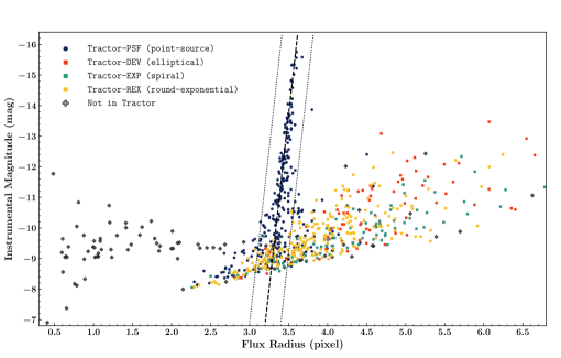
We developed a morphological classifier to carry out the source selection in sparse-flavor SFFT. The classifier was initially proposed for PSFEx (Bertin, 2011), which enables PSFEx to select a subset of point sources for constructing the PSF model. Given a photometry catalog generated by SEXTRACTOR (Bertin & Arnouts, 1996), one can draw a figure of instrumental magnitudes (SEXTRACTOR catalog value MAG_AUTO) against flux radius (SEXTRACTOR catalog value FLUX_RADIUS) for all detected photometry objects. Generally, bright point sources tend to stay around a nearly vertical straight line on this figure. PSFEx leverages the statistical feature to select appropriate samples to establish the PSF model. Although the goal of source selection for sparse-flavor SFFT is not entirely aligned to that for PSFEx, it inspires us to make the selection based on SEXTRACTOR parameters and their statistical characters.
To demonstrate the source selection criterion in sparse-flavor SFFT, we show an example of an individual DECam (Honscheid & DePoy, 2008) image in Figure 1. By contrast, the SEXTRACTOR photometry catalog of this image is cross-matched with the Tractor catalog from Legacy Survey (Blum et al., 2016), which offers their own fitted morphological types. As shown in Figure 1, the point sources and extended sources form two conspicuous branches, which intersect at the faint end but become well-separated towards the bright side. According to the Tractor types, the branch with a nearly vertical orientation primarily comprises point-like sources with Tractor type PSF, while the extended sources with Tractor types DEV, EXP, REX are likely to be found in the other branch that sprawls out horizontally. Moreover, the discrete gray dots represent the objects that cannot be found in the Tractor catalog, which are casual detections such as cosmic rays. SFFT uses Hough Transformation (Hough, 1959) to identify the straight line surrounded by the branch of point sources. The figure is first pixelized by counting the number of objects in each small grid. Hough Transformation is applied so that we can search for the strongest line feature with vertical orientation. The thin belt-like region around the detected straight line with a fixed width is referred to as point-source-belt. In SFFT, the parameter -BeltHW describes the belt half-width (default value is 0.2). With this terminology, it is easier to describe the specific selection criteria.
For the source selection, sparse-flavor SFFT will first generate a SEXTRACTOR photometry catalog for reference image and science image, respectively. A source is selected if it lies in point-source-belt or out of point-source-belt from the right side for both images. The extended sources in the field are not excluded, as SFFT can use both stars and galaxies to derive the solution for the matching kernel. However, typical cosmic rays and the faintest astronomical sources will be discarded. Given that each pixel of selected samples is equally weighted no matter bright or faint in SFFT, rejecting the noisiest subset should be appropriate in our framework. Furthermore, SEXTRACTOR has been configured to only output the objects with SEXTRACTOR catalog value FLAG being zero. Namely, this guarantees that the saturated sources and blending objects (relatively rare in sparse fields) are not in the selection.
Significant variable sources in the field should be further rejected. SFFT cross-matches the photometry catalogs of the input image-pair, then calculates the difference in instrumental magnitude for each matched object. The outliers of the distribution of magnitude difference indicating violent brightness change will be discarded from the initial set of selection. In SFFT, the outliers are identified by the threshold parameter -MAGDTHRESH (default value is 0.12 mag). The survived selection set is applied for the image-masking in sparse-flavor SFFT. The outlier rejection is usually sufficient enough for a successful image subtraction, but one is also allowed to further refine the automatic selection by removing the known but not recognized variables and transients. Unlike HOTPANTS, SFFT does not enclose each source of the selection within a fixed-size rectangle stamp. Instead, we employ the detection mask of SEXTRACTOR (check-image SEGMENTATION generated by SEXTRACTOR) to define the pixel domain of each selected source. Finally, the pixels not in any pixel domain will be masked by a constant of zero.
3.3 Implementation of SFFT Subtraction
The next step is to perform subtraction with the unmasked and the masked image-pairs, in the same way for the two flavors. We implemented the subtraction algorithm in CUDA following the mathematical reasoning in Section 2.2.
There are a few free parameters in this process. In Section 2.2, the spatial variation of the convolution kernel was modeled as a polynomial form of degree . Similarly, the differential background is assumed to be a polynomial with degree . In SFFT, the two free parameters correspond to -KerPolyOrder and -BGPolyOrder, respectively. The default values of the two parameters are 2. Another parameter that should be specified is the pixel size of the convolution kernels. The default way is to determine kernel size as seeing-related, i.e., the kernel half-width is calculated as , where the ratio -KerHWRatio is a free parameter of SFFT and is the worse seeing of the input image-pair. The last free parameter -ConstPhotRatio is boolean, which controls whether SFFT subtraction is subject to a constant photometric ratio or not. The default value of this parameter is True that assumes the input image-pair has been well-calibrated. Setting the parameter to be False means the photometric ratio will also become a polynomial form of degree -KerPolyOrder.
4 Examples of Image Subtraction with SFFT
We show examples of SFFT applied to observations from five different telescopes. These data correspond to a diverse range of characteristics. The technical specifications of the instruments are given in Table 1. To test the two flavors of SFFT, we use ZTF (Bellm et al., 2018), AST3-II (Yuan et al., 2014), and TESS (Ricker et al., 2015) data as examples of crowded fields. Also, the observations from DECam and TMTS with abundant isolated stars are selected as representatives of sparse fields.
The ZTF (Bellm et al., 2019) and AST3-II (Wang et al., 2017; Yuan et al., 2014) data are images of the nearby galaxies M31 and the Large Magellanic Clouds (LMC), respectively. The two wide-field survey telescopes have the same pixel sampling but point to a different hemisphere. We additionally test SFFT with TESS (Ricker et al., 2015) images with a vastly different pixel scale of 21.0 arcsec/pixel where PSF is severely under-sampled. All of these selected observations could be seen as signal-dominated cases so that subtraction tests on them are conducted by the crowded-flavor SFFT.
The DECam and TMTS data were acquired for extragalactic transient surveys (Mould et al., 2017; Zhang et al., 2020). The DECam data are from deep surveys with a large number of isolated point sources and extended galaxies, while the TMTS data are from a shallow nearby survey that recorded plenty of point sources. TMTS has a larger pixel scale than DECam, but its PSF is not under-sampled, unlike TESS. For these observations, the observed stellar objects are generally isolatedly distributed in the field, making it possible to apply the source selection described in Section 3. We use sparse-flavor SFFT for the subtraction tests on DECam and TMTS.
Through this section, SFFT always uses the default configuration of free parameters described in Section 3, which are summarized in Table A1, even though the two sets of images differ drastically. The detailed information for the test data used in this section is presented in Table B. In the context, we will highlight the alias names of the test images in italic. All input image-pairs for image subtraction have been registrated by SWarp (Bertin, 2010) with LANCZOS3 resampling function. For the input images of sparse-flavor SFFT, we have modeled and subtracted their sky using SEXTRACTOR with a mesh size of 64 64 pixels.
4.1 Crowded Fields
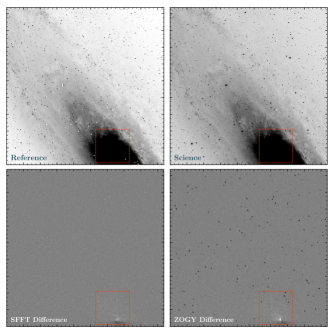
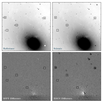
By design, SFFT does not require isolated sources to solve the image matching. In crowded fields where few or no isolated stars are present, SFFT can perform exceptionally well. The ZTF test images are downloaded from ZTF Data Release 3 222https://www.ztf.caltech.edu/page/dr3, covering the nearby galaxy M31. Figure 2 and Figure 3 show the subtraction performance of both the SFFT and ZOGY method, with a wider view and a close-up view on the galaxy core, respectively.
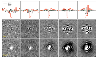
The difference image generated by SFFT is much cleaner than the ZOGY approach, as indicated by the lower panels of the two figures. One can also notice that the difference image by the ZOGY method appears to have a bias seemingly due to the photometric mismatch of image subtraction. This guess is confirmed in Figure 4 that analyses the flux residuals of five field stars near the galaxy core. ZOGY subtraction uniformly remains negative net flux for these samples, suggesting an improperly-estimated photometric ratio between reference and science image. By contrast, SFFT does not have the same problem. Unlike ZOGY, the photometric ratio (a constant in our default configuration, i.e., ) in SFFT is straightforwardly solved from the linear system, rather than an extra value calculated by some other photometric process.
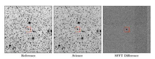
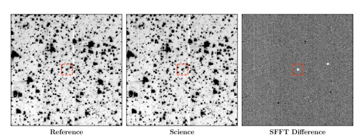
Figure 5 and Figure 6 show SFFT subtraction performance on LMC observations of the Antarctica telescope AST3-II and test data from space-based TESS 30min-cadence Full Frame Images (FFIs), respectively. A known variable star of RRAB type is easily identified at the image center for both cases. It illustrates how the flux variability can be effectively captured by SFFT subtraction from the densely packed fields.
4.2 Sparse Fields
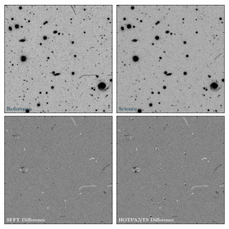
It is also essential to investigate the performance of SFFT subtraction on the ordinary sparse sky fields that are more common in extragalactic transient surveys. For comparison, we additionally employed the widely-used image subtraction software HOTPANTS as a baseline method. As one of specific implementations of Alard & Lupton (1998), HOTPANTS adopts Gaussian basis functions to construct the convolution kernel. In real space, the use of DBFs has been shown to yield better performance than Gaussian basis functions in terms of photometric accuracy (Albrow et al., 2009). Here we present the comparisons to HOTPANTS to confirm that the SFFT, though working in Fourier space, will still inherit the advantage of DBFs over Gaussian basis functions. The parameters of HOTPANTS used for this section are listed in Table A2. Recall that sparse-flavor SFFT restricts the calculations of convolution kernels on a pre-selected set of sources, this source list used by SFFT will be shared by HOTPANTS for the sake of fairness. Besides, both methods always apply the consistent size of convolution kernels and use the same polynomial degree of spatial variation for image subtraction. We selected 25 DECam observations with the same pointing but diverse seeing conditions from our DECamERON survey (Mould et al., 2017) (see Table B). With the set of DECam images, we conduct two types of tests to check the subtraction cleanness and photometric accuracy, respectively.
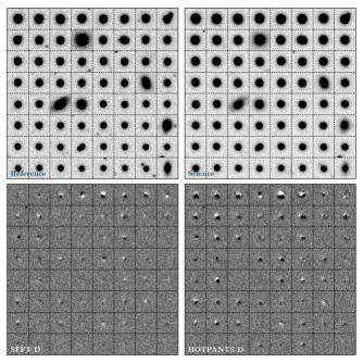
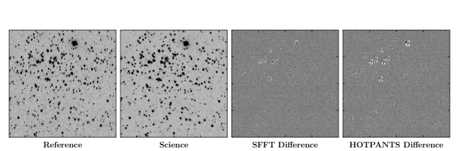
For the subtraction cleanness test, we use the image DECam-SREF as the shared reference, having the best seeing among all of them. The remaining 23 images aliased by initial DECam-OBS are regarded as science images in this test. Image subtractions are performed for the sequence of science images with a shared reference using sparse-flavor SFFT and HOTPANTS, respectively. An example of the subtraction results is shown in Figure 7 from the observation DECam-OBS02f. For both methods, the calculations involved in parameter-solving have been restricted to the same pre-selected sources, and the minimization aims at optimal subtraction on these sources as clean as possible. It is useful to give a close-up view of subtraction performance specifically for the selection. For each image in Figure 7, we cut a small thumbnail image around each selected source and combine the cutouts into a grid to be a new synthetic image, as shown in Figure 8. Note that the source selection, in this case, is more than 1100, so we only exhibit a subset of size 64 from the bright end of the complete set for a clear display. One can notice that the most conspicuous subtraction-induced artifacts have a dipole-like pattern which is especially prominent for the bright sources. The pattern can be found in both difference images, but much less profound in SFFT subtractions than in HOTPANTS subtractions. It is an expected improvement as the SFFT kernel solution with DBFs allows more degrees of freedom than HOTPANTS using Gaussian basis functions.
To further verify such an improvement is real in a statistical sense, here we defined a naive quantifiable metric to describe the subtraction cleanness and show the performance comparisons with the test data. Note that the subtraction-induced artifacts on difference images are usually detectable by SEXTRACTOR like other real transient and variable objects. Generally, a huge number of artifacts in transient surveys will survive until an AI-based stamp classifier recognizes them. This fact makes it possible to use a simple dichotomous metric to describe the subtraction cleanness. A given source is either clean-subtracted or not according to the existence of SEXTRACTOR detection of its subtraction residuals. Now we can investigate how the probability of clean-subtraction for a given set of sources is related to the employed image subtraction method. For transient surveys, it is essential to probe the subtraction performance over the galaxies in the field, which are potential hosts of transient events. When a transient emerges at a position very close to its host galaxy core, the subtraction-induced artifacts from the galaxy can severely hinder the discovery and photometric measurement of the transient.
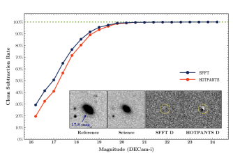
Our deep DECam observations in the test (3 square degrees, down to 23.5 mag in i-band) have covered a vast number of galaxies with various morphological types. It is interesting to make statistics for the probability of clean-subtraction for those sources identified as extended galaxies (i.e., Tractor morphological types DEV, EXP, and REX) in the Legacy Survey (Blum et al., 2016). The check radius from the galaxy core for searching subtraction-induced artifacts using SEXTRACTOR is specified as 11 pixels ( 2 times median FWHM for DECam). Figure 9 shows the rate of clean-subtraction as a function of the magnitude of the examined galaxy. As expected, the brighter galaxies have a higher probability of leaving detectable subtraction-induced artifacts. However, the SFFT method is more likely to achieve clean-subtraction than HOTPANTS.
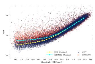
For the photometric accuracy test, we use the image DECam-PTAR as the PSF target, which has a median level seeing among all selected DECam observations. The remaining 23 images aliased by initial DECam-OBS are convolved to achieve homogeneous PSF using sparse-flavor SFFT and HOTPANTS, respectively. We derive the light curves of the field stars by conducting photometry on the sequence of convolved images with a fixed aperture. The photometric accuracy measured by the light curves can work as a metric to assess the PSF matching quality. We investigate the aperture photometry of the point sources classified as Tractor morphological type PSF. Figure 10 shows the RMS error of the derived light curves as a function of the star brightness. As the photometric uncertainty from SFFT is systematically lower than that from HOTPANTS especially at the bright end, the improvement in PSF matching is again confirmed.
Figure 11 shows an example with TMTS data. The subtraction artifacts generated by SFFT and HOTPANTS are not identical. HOTPANTS produces relatively circular and symmetric patterns, while SFFT shows more random residuals. This obviously originates from the different base kernel construction in SFFT and HOTPANTS. SFFT uses a -basis kernel which is more flexible, while HOTPANTS utilizes Gaussian functions which possess a higher intrinsic symmetry about the kernel center.
5 Computational Performance of SFFT
The most remarkable feature of SFFT is that the image subtraction in Fourier space can be efficiently parallelized in GPU devices. With the simplification described in Appendix B, we have reduced the computation-intensive kernel determination as discrete Fourier transforms (DFTs) and element-wise matrix operations, which are exceptionally suitable for GPU graphic multi-processors. This section will show the excellent computing performance of the SFFT algorithm in comparison with several existing image subtraction methods, including HOTPANTS, ZOGY333https://github.com/pmvreeswijk/ZOGY, and PyTorchDIA444https://github.com/jah1994/PyTorchDIA. Note that the comparisons only focus on the limited specific implementations of image subtraction algorithms. One should not overinterpret the computing costs given in this section to represent the best possible computational performances of the general algorithms. Unless specified otherwise, the parameters of those softwares used for this section are listed in Tables A1,A2,A3,A4.
| Method | Time Cost on Preprocessing (sec) | Time Cost on Subtraction (sec) | |||||
| Intel E5 | AMD EPYC | Intel E5 | AMD EPY | Tesla V100 | Tesla A100 | ||
| CPU | CPU | CPU | CPU | GPU | GPU | ||
| SFFT | 5.75 0.26 | 3.35 0.15 | - | - | 1.61 0.10 | 0.97 0.06 | |
| PyTorchDIA | 0.11 0.01 | 0.16 0.07 | - | - | 15.87 3.25 | 6.45 1.36 | |
| HOTPANTS | 4.37 0.85 | 2.43 0.39 | 26.39 8.50 | 15.39 3.49 | - | - | |
| ZOGY | 63.59 6.42 | 42.28 3.74 | 62.83 9.16 | 41.01 5.25 | - | - | |
It is useful to demonstrate the computing performance of the image subtraction methods by testing them with a variety of data on different computation platforms. We select a set of testing input data with diverse image sizes, seeing conditions, and sky areas. The tests are performed on two computing servers with different hardware configurations. One server (denoted by ) is equipped with Intel(R) Xeon(R) CPU E5-2630 (2.20 GHz) and one NVIDIA Tesla V100 GPU, while the other server (denoted by ) has more advanced configurations with AMD EPYC CPU 7542 and one NVIDIA Tesla A100 GPU. Note that the time spent on preprocessing steps can also be considerable. We additionally record the computing cost of the pre-subtraction procedures in our tests. In this section, we conduct two types of tests using TMTS data and DECam data, respectively.
To explore the relationship between the computing time and input image size, we extract sub-images of different sizes from the original TMTS image-pair (i.e., TMTS-REF and TMTS-SCI). We then perform image subtractions for the trimmed image-pairs on the two servers using the four tested methods. For SFFT, HOTPANTS and PyTorchDIA, in order to test if the computational cost is sensitive to the size of the convolutional kernel, we run the image subtractions repeatedly with a specified kernel size from 15 to 25 pixels in each run (six runs in total).
Figure 12 shows the computing time on the preprocessing as a function of input image size. In general, larger input images consume more computing time on preprocessing. Among the tested methods, ZOGY requires the longest preprocessing time. For ZOGY, the preprocessing is composed mainly of fitting the PSF models for input images and calculating their flux ratio as well as the astrometric registration noises. The preprocessing time of SFFT and HOTPANTS are comparable and much shorter than ZOGY. For these two methods, the goal of the pre-subtraction procedures is to select an optimal set of sources for kernel determination. Like in Section 4.2, we have forced HOTPANTS to use the pre-selected set given by SFFT following Section 3.2. Note that SFFT needs further to perform an image-masking based on the pre-selected set while HOTPANTS does not, that is why the preprocessing time of SFFT is slightly longer than HOTPANTS. For PyTorchDIA, the preprocessing only contains reading the input FITS images. Thus, it can achieve minimal preprocessing time. We note that the robust loss function used in PyTorchDIA is designed to be insensitive to the distraction-sources, as a result, no source selection or image-masking is involved in PyTorchDIA.
Figure 13 presents the computing time on the image subtraction versus the input image size. Unsurprisingly, larger images generally require more computing time for subtraction. The computing speeds for HOTPANTS and ZOGY are broadly comparable, with a typical cost of 40-90s for 4K images. By contrast, the GPU-powered method PyTorchDIA brings considerable speed-up. For 4K images, the computing time is around 30s and 10s on the server and , respectively. Note that PyTorchDIA only solves a spatially invariant kernel while other tested methods can accommodate spatially varying PSF. Remarkably, SFFT is almost an order of magnitude faster than PyTorchDIA. For 4K images, the computing time is close to 4s and 1s on the server and (), respectively. As shown in Figure 13, the subtraction speed of SFFT is less affected by the kernel size compared to HOTPANTS and PyTorchDIA.
The second type of test aims to explore the computing expense on a set of images with diverse seeing conditions covering different sky areas. We randomly select 100 CCD images from the 23 DECam observations aliased by initial DECam-OBS (see Table B). Note that one DECam exposure produces 62 CCD images, each with a size of 20464094 pixels. As shown in Table B, the DECam data were obtained under varying seeing conditions. Although the DECam exposures listed in Table B have similar telescope pointing, the arbitrarily selected CCD images can, to some extent, cover a variety of distributions of the observed stellar objects. In this test, the selected 100 images are regarded as science images, and we use the corresponding CCD images of DECam-SREF as their reference images. We perform image subtractions for the 100 image-pairs on the two servers using the four tested methods. Unlike the above test, we do not specify a given kernel size but leave it automatically determined according to the seeing condition. Table 2 summarizes the time costs on preprocessing and image subtraction for the tested DECam dataset. The results are broadly consistent with the first test. Again, SFFT shows a distinct advantage in the subtraction speed over other tested methods. Given image size, SFFT is the most stable method on subtraction time, with a percentage variation (the typical value is for other methods).
We note that the software HOTPANTS also allows users to perform image subtraction without a pre-selected source list. In such an automatic mode, HOTPANTS will accomplish the source selection using its built-in functions. One may wonder if the automatic mode can be faster than the manual mode used in this paper. Hence, we additionally perform the image subtraction on the 100 image-pairs using the automatic mode HOTPANTS. It turns out that the total time (preprocessing plus subtraction) for the two modes is very close, with the automatic mode having a slightly higher variation.
For the crowded fields, the computational cost of SFFT will not rise to a level higher than the cost shown in this section. For preprocessing, crowded-flavor SFFT involves much simpler operations than spase-flavor (see Section 3.1). On the other hand, signal-dominated input images will not prolong the computing time on image subtraction in Fourier space.
| HOTPANTS | Total Time Cost (sec) | |||
| Mode | Intel E5 | AMD EPYC | ||
| Manual (this work) | 30.76 8.81 | 17.82 3.62 | ||
| Automatic | 30.75 10.54 | 17.71 4.40 | ||
6 Limitations and Future Works
| Method | Convolution Kernels | Accommodate Spatial Variations | |||||
| Gaussian-function | -function | Regularized | Convolution | Photometric | Differential | ||
| basis | basis | Kernel | Kernels | Scale Factor | Background | ||
| SFFT | ✗ | ✓ | ✗ | ✓ | ✓ | ✓ | |
| PyTorchDIA | ✗ | ✓ | ✗ | ✗ | ✗ | ✓ | |
| HOTPANTS | ✓ | ✗ | ✗ | ✓ | ✗ | ✓ | |
| ZOGY | - | - | - | ✓ | ✓ | - | |
| Method | Kernel Determination | ||||||
| Require PSF | Require Isolated | Rely on Rectangle | Weighting by | Construct Least | Symmetric to | ||
| Knowledge | Objects | Sub-areas | Pixel Noise | -squares Matrix | Image Exchange | ||
| SFFT | ✗ | ✗ | ✗ | ✗ | ✓ | ✗ | |
| PyTorchDIA | ✗ | ✗ | ✗ | ✓ | ✗ | ✗ | |
| HOTPANTS | ✗ | ✓ | ✓ | ✗ | ✓ | ✗ | |
| ZOGY | ✓ | ✓ | ✓ | - | ✗ | ✓ | |
| Method | Preprocessing before Subtraction | Computing Performance of Subtraction | |||||
| Stamp Selection | PSF | Calculate | Implemented | Built-in CPU | Speed Sensitive | ||
| /Image Masking | Modeling | Flux Ratio | for GPU | Multithreading | to Kernel Size | ||
| SFFT | ✓ | ✗ | ✗ | ✓ | - | ✗ | |
| PyTorchDIA | ✗ | ✗ | ✗ | ✓ | - | ✓ | |
| HOTPANTS | ✓ | ✗ | ✗ | ✗ | ✗ | ✓ | |
| ZOGY | - | ✓ | ✓ | ✗ | ✓ | - | |
To get a clear picture of the current SFFT and find its limitations, we summarize a variety of features from different perspectives for SFFT and other existing image subtraction methods, including PyTorchDIA, HOTPANTS and ZOGY in Table 4. Although a general algorithm (e.g., Alard & Lupton, 1998) can have multiple existing implementations, the scope of the comparisons in Table 4 is restricted: we have only considered a specific implementation for each algorithm. Some characteristics of a specific implementation may not necessarily be the intrinsic features of its underlying algorithm (see the note attached to Table 4).
Although SFFT uses the state-of-the-art DBFs as kernel basis functions, the current version does not contain an effective mechanism to aginst the overfitting problem of DBFs. In future work, we may try to incorporate existing solutions into SFFT, e.g., Becker et al. (2012); Bramich et al. (2016); Masci et al. (2017). Moreover, unlike Alard & Lupton (1998); Bramich (2008); Hitchcock et al. (2021), the kernel determination in SFFT is not weighted by pixel noise, which may introduce a possible bias towards the brighter pixels. It looks tricky to design a weighting scheme in Fourier space. Note that some practical implementations, including HOTPANTS and Miller et al. (2008), also ignore the pixel weights in kernel determination.
As discussed in Zackay et al. (2016), the approach proposed by Alard & Lupton (1998) is not symmetric, i.e., changing the convolution direction of image subtraction will generally result in inconsistent difference images. Consequently, SFFT has some limitations inherited from the nature of this kind. In particular, when the direction matches an image to another one with better seeing, the deconvolution effect makes its way into the subtraction to amplify the noise and strengthen noise correlation on the difference image. In many cases, one can steer clear of the deconvolution effect by simply adjusting the direction. However, this strategy is not a panacea; e.g., it may be insufficient when the observations have elliptic-like PSF with varying orientations (Zackay et al., 2016).
Another limitation of the current SFFT is related to the computing cost of preprocessing. The image-masking scheme of SFFT introduced in Section 3 provides a safe and generic approach that has been proved to be reliable through extensive tests by multiple transient surveys. However, its computing cost might become a potential encumbrance for those projects that pursues extremely rapid transient detection. Fortunately, there is ample space for speed-up in a given survey program. One can modify the SFFT code to design a particular image-masking function for optimizing its overall computing expense. For example, the SEXTRACTOR catalogs used for the source selection can be provided by preceding modules (e.g., astrometric calibration) in the pipeline. When processing time-series data taken from the same pointing, one can skip the repeated photometry for the shared reference image to save the preprocessing time. One may also consider using a single pre-defined mask (fixed or seeing-related) for all images in the time series. We note that PyTorchDIA can take very little time on preprocessing as it designs a specific loss function insensitive to outlying values, which provides an alternative to suppress the impact from distraction-sources amid the kernel determination.
In the current implementations of SFFT, the subtraction has two flavors that make image-masking in different ways. However, there is no built-in discriminator for sparse fields and crowded fields in SFFT. One may specify the adopted flavor for each field to be processed. In future work, we may consider developing a more unified way to conduct image-masking rather than dividing the observations into two subgroups. Besides, the limited memory amount of GPU devices can constrain the applicability of the GPU-based SFFT to very large images. To allows for large image cases, we have provided a Numpy-based backend for SFFT without GPU requirement. This is also helpful for users who do not have available GPU resources.
7 Summary and Conclusions
SFFT is a novel image subtraction algorithm formulated in Fourier space. Like in the classic framework of Alard & Lupton (1998), SFFT addresses the PSF discrepancy between two images by the convolution with pixelized kernels that are decomposed into pre-defined basis functions. In our work, we adopted the -function basis proposed by Miller et al. (2008) for kernel flexibility and minimal hyper-parameters. SFFT solves the least-squares problems of image subtraction in the Fourier domain, and it allows for space-varying PSF, photometric scaling, and sky background modeling across the entire field-of-view. In particular, SFFT can reduce the computation-intensive kernel determination to FFTs and element-wise matrix operations. By leveraging CUDA-enabled GPU acceleration, SFFT empowers a great leap forward in computational performance of astronomical image subtraction with around one order of magnitude speed gain.
We demonstrated in this paper the power of the method on real astronomical images taken by a variety of telescopes. We show that SFFT can accommodate imaging data with diverse characteristics, including sparse fields, crowded fields, and under-sampled PSFs. The examples of SFFT for image subtraction are presented in Section 4. We confirm that SFFT yields a high quality of PSF-matching when compared with the widely-used image subtraction software HOTPANTS using Gaussian kernel basis for models of the PSFs. A comprehensive investigation of the computing performance of SFFT is presented in Section 5. We find that SFFT is not only faster compared to other existing image subtraction methods but is also more stable and efficient.
We also explored the limitations of the current SFFT implementation in Section 6. One prominent weakness of the current SFFT is that the kernel solutions may suffer from the overfitting problem due to the high degree of freedom of DBFs. A few approaches have been proposed to alleviate the overfitting issue of DBFs, e.g., regularizing the kernel solutions (Becker et al., 2012). However, the DBFs employed by the current SFFT are unregularized. The regularization techniques will be included in future works. In the meantime, proper image masking is required in the current version of SFFT to identify the pixels that are not correctly modeled by SFFT. In principle, SFFT also provides a generic and robust function to perform preprocessing of the data, which has been extensively tested with data from various transient surveys. In contrast to the high speed of the image subtraction, however, the computing performance of the generic preprocessing is less remarkable. Given a particular time-domain program, we believe there is plenty of room for further optimization of the computing expense on the preprocessing.
We conclude that SFFT has the potential to be the optimal image subtraction engine for future time-domain surveys with massive data flows that require differential image subtractions for transient detection and precision differential photometry.
Appendix A The Approximation in SFFT
Here we will prove the approximation applied to Equation (10). Given any image R and a kernel Q, where Q has a much smaller size than R as it is in most astronomical applications.
| (A1) |
Writing the Left Hand Side (LHS) and Right Hand Side (RHS) as follows,
| (A2) |
| (A3) |
Note that the indices of kernel are modified with origin at its center pixel, and the subscript is employed to indicate the periodic extension.
For and , is a vector within the image frame and for nearly all possible and .
| (A4) |
For the particular case , it becomes a rigorous equation rather than an approximation.
Appendix B Calculation Simplification
The -function basis facilitates further simplifications. Equation (19) will be re-expressed as
| (B1) |
where
| (B2) |
Equation (24) at the right-hand-side becomes
| (B11) |
where
| (B12) |
Appendix C Noise Decorrelation
| Parameter | Value | Note | Comment | |
|---|---|---|---|---|
| -BeltHW | 0.2 | Half-width of the point-source-belt | only for sparse-flavor | |
| -MAGD_THRESH | 0.12 | Outlier threshold to reject variable sources (mag) | only for sparse-flavor | |
| -KerPolyOrder | 2 | Spatial order of kernel variation | - | |
| -BGPolyOrder | 2 | Spatial order of background variation | - | |
| -KerHWRatio | 2 | The ratio between seeing and convolution kernel half-width | - | |
| -ConstPhotRatio | True | Constant photometric ratio between reference and science | - |
Note. — For PyTorchDIA, the kernel regularization has been mentioned in Hitchcock et al. (2021) whereas no regularization has been implemented in the software PyTorchDIA; For HOTPANTS, the kernel determination relies on a set of stamps encompassing isolated objects. Note that requiring isolated objects is not a feature of Alard & Lupton (1998). Moreover, pixel noise is not used in the matrix calculation in HOTPANTS though formulated in Alard & Lupton (1998); For ZOGY, all the convolutions involved in image subtraction are determined by pre-calculated PSFs. Generally, constructions of the PSF models are based on a sample of rectangle sub-images (e.g., SExtractor VIGNETS) centered at isolated bright point sources.
Like in other subtraction methods emanated from Alard & Lupton (1998), SFFT will introduce correlated errors on the difference image through the convolution process. For the cross-convolution approach, Zackay et al. (2016) has proved that one can whiten the difference image by one convolution with a decorrelation kernel. Later, Reiss & Lupton (2016) presented a noise decorrelation strategy for image subtraction in the framework of Alard & Lupton (1998). Here we extend to a more general case. That is, the subtraction can be performed with images constructed from the average or median co-addition of individual observations, and the original images are preprocessed by convolutions to match their PSFs before the co-additions.
The following derivation does not consider the spatial variation of convolution kernels across the field-of-view. However, it is appropriate to perform the operation by splitting the images into smaller segments to minimize the effect of PSF variation on correlated background noise. Likewise, the spatial variation of the background map for the input images is not considered. Note that a constant map has nothing to do with the noise correlation. Therefore, it is appropriate to assume that all the input images have zero mean background in our derivation. Note that noise correlation caused by resampling for image alignment and drizzling is not considered here, as such operations cannot be simplified as convolution, and it is not easy to formulate how these procedures affect the statistical properties of the noise. Finally, we assume that the noise of the original images before convolution to be uncorrelated Poisson noise.
Given science images with being integers from 0, , and reference images with being integers from 0, , respectively. We consider the generic case of subsequent average or median co-additions produce the stacked science and reference images. The image subtraction employed to obtain the final difference image is given by
| (C1) |
For simplicity, the convolution kernels and for PSF-homogenisation are divided by number of science () and reference () images and , respectively. Assuming that a decorrelation kernel exists which can whiten the noise of , we can calculate using the equation where .
The covariance matrix of in Fourier space can be written as
| (C2) |
where and are the image dimensions in and directions, respectively, and and are pixel indices of the image frame.
The Foruier Transform of the decorrelation kernel can be derived by setting ,
| (C3) |
The final solution to should be conjugate symmetric to ensure its inverse Fourier Transformation to be real. Here we consider the most straightforward solution with being a real function only, that is
| (C4) |
Note is the desired noise of decorrelated difference image. In principle, it should be set to be as close as possible to the true background in regions free of astronomical objects. In practice, this normalization can also be set by requiring the decorrelation procedure to preserve the flux zero-point of the images. In the latter case, SFFT simply normalizes the decorrelation kernel to have a unit kernel sum.
There is a major difference between SFFT and ZOGY (Zackay et al., 2016) for noise decorrelation, although they share the same statistical principles. In ZOGY, convolution kernels for co-addition and subtraction are tied to the PSFs of the images. SFFT does not need to model the PSFs for the images and for the noise decorrelation process. Only the match kernels , , and are needed for SFFT. This can be even more convenient for images with simple co-additions of original observations without matching the PSFs, such as observations taken under stable seeing conditions, only the match kernel is needed for SFFT, and no PSF construction is necessary.
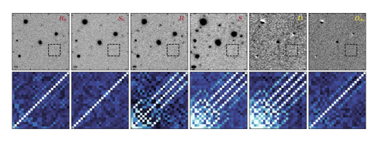
We select ten DECam images from Table B for testing the performance of noise decorrelation. The generic case of image subtraction follows Equation (C1), with {, , , , } = {DECam-OBS18a, DECam-OBS18b, DECam-OBS18c, DECam-OBS18d, DECam-OBS18e} being the individual reference images, and {, , , , } = {DECam-OBS04a, DECam-OBS04b, DECam-OBS04c, DECam-OBS04d, DECam-OBS04e} being the individual science images. All the images have been astronomically aligned to by SWarp. We create the stacked reference image by median co-addition of the five individual reference images with PSF homogenization matching to . Similarly, the stacked science image is the median coadd of the five individual science images after matching their PSFs to . The final subtraction is performed between the stacked reference and stacked science image. Noise decorrelation for the difference image is conducted by convolving the decorrelation kernel calculated by Equation (C4). As the spatial variation has been ignored, here, the example only focuses on a small area around the supernova candidate AT 2018fjd discovered in DECamERON survey (Hu et al., 2018).
We trace the background pixel correlation along with the coadd and subtraction processes, shown in Figure 14. Note that image alignment can also introduce pixel correlation via a localized resampling function (LANCZOS3 function of SWarp in this case). One can notice that the pixel correlation in resampled image is already slightly higher than un-resampled image . The correlation is increased drastically in co-added images as multiple convolutions for PSF homogenization come into play in this process. It becomes even stronger after the final subtraction. Nevertheless, our decorrelation scenario can effectively reduce the noise correlation on the final difference image to a quite low level comparable with that of a resampled individual image .
| Parameter | Value | Note | |
|---|---|---|---|
| -r | Convolution kernel half-width (pixel) | ||
| -rss | Substamp half-width (pixel) | ||
| -nsx | NX / 200 | Image segmentation of stamps (x axis) | |
| -nsy | NY / 200 | Image segmentation of stamps (y axis) | |
| -ko | 2 | Spatial order of kernel variation | |
| -bgo | 2 | Spatial order of background variation | |
| -tu | saturation recorded in reference header | Upper valid flux of the reference image | |
| -tl | Lower valid flux of the reference image | ||
| -iu | saturation recorded in science header | Upper valid flux of the science image | |
| -il | Lower valid flux of the science image |
Note. — is the worse seeing measured from the input image-pair. Note the ratio of 2 in parameter is consistent with the default configuration of SFFT (see -KerHWRatio). The parameters -ko and -bgo are equivalent to SFFT paramters -KerPolyOrder and -BGPolyOrder, respectively. The symbols NX and NY indicate the image size along x axis and y axis, respectively. sky and skysigma describe the sky background measured by MMM algorithm. The HOTPANTS configurations here largely refer to those in iPTF image subtraction pipeline (Cao et al., 2016).
| Parameter | Value | Note | |
|---|---|---|---|
| -subimage_size | 256 | Size of subimages (pixel) | |
| -subimage_border | 32 | Border around subimage to avoid edge effects (pixel) | |
| -fratio_local | F | Flux ratio from subimage (T) or full frame (F) | |
| -psf_poldeg | 2 | Polynomial degree for PSF spatial variation | |
| -size_vignet | 49 | Size of the SExtractor VIGNETS for PSF construction | |
| -nthreads | 32 | Number for CPU multithreading |
| Parameter | Value | Note | |
|---|---|---|---|
| -loss_fn | robust | loss function (robust or Gaussian) | |
| -flat | 1 | Initialization value of the convolution kernel | |
| -ks | Kernel size | ||
| -poly_degree | 2 | Polynomial degree for background fit |
Note. — is the worse seeing measured from the input image-pair.
| Instrument | File Alias | File Name | Exposure Time | FWHM | 5 Lim. Mag | |
|---|---|---|---|---|---|---|
| (s) | (arcsec) | (mag) | ||||
| ZTF | ZTF-REF | ztf001735zgc01q2refimg | 1200 | 2.02 | 22.89 | |
| ZTF | ZTF-SCI | ztf20180705481609001735zgc01oq2sciimg | 30 | 1.80 | 20.68 | |
| AST3-II | AST-REF | a0331.94 | 60 | 2.41 | - | |
| AST3-II | AST-SCI | a0405.162 | 60 | 2.96 | - | |
| TESS | TESS-REF | tess2018258205941-s0002-1-1-0121-sffic.001 | 1440 | 36.95 | - | |
| TESS | TESS-SCI | tess2018258225941-s0002-1-1-0121-sffic.001 | 1440 | 36.89 | - | |
| DECam | DECam-SREF | c4d180806052738ooiiv1 | 330 | 0.85 | 24.35 | |
| DECam | DECam-PTAR | c4d150821001224ooiiv1 | 330 | 1.40 | 22.73 | |
| DECam | DECam-OBS18a | c4d160818043331ooiiv1 | 330 | 1.04 | 23.28 | |
| DECam | DECam-OBS18b | c4d160818020339ooiiv1 | 330 | 1.07 | 23.35 | |
| DECam | DECam-OBS18c | c4d160818030325ooiiv1 | 330 | 0.96 | 23.45 | |
| DECam | DECam-OBS18d | c4d160818053313ooiiv1 | 330 | 1.12 | 23.09 | |
| DECam | DECam-OBS18e | c4d160818065148ooiiv1 | 330 | 1.01 | 23.32 | |
| DECam | DECam-OBS02a | c4d180802052807ooiiv1 | 330 | 1.38 | 23.40 | |
| DECam | DECam-OBS02b | c4d180802055800ooiiv1 | 330 | 1.31 | 23.55 | |
| DECam | DECam-OBS02c | c4d180802062754ooiiv1 | 330 | 1.22 | 23.60 | |
| DECam | DECam-OBS02d | c4d180802065746ooiiv1 | 330 | 1.41 | 23.33 | |
| DECam | DECam-OBS02e | c4d180802072740ooiiv1 | 330 | 1.21 | 23.58 | |
| DECam | DECam-OBS02f | c4d180802075732ooiiv1 | 330 | 1.29 | 23.62 | |
| DECam | DECam-OBS02g | c4d180802085719ooiiv1 | 330 | 1.24 | 23.55 | |
| DECam | DECam-OBS02h | c4d180802092739ooiiv1 | 330 | 1.35 | 23.42 | |
| DECam | DECam-OBS04a | c4d180804092331ooiiv1 | 330 | 1.41 | 23.50 | |
| DECam | DECam-OBS04b | c4d180804052409ooiiv1 | 330 | 1.37 | 23.62 | |
| DECam | DECam-OBS04c | c4d180804055402ooiiv1 | 330 | 1.57 | 23.43 | |
| DECam | DECam-OBS04d | c4d180804075344ooiiv1 | 330 | 1.36 | 23.61 | |
| DECam | DECam-OBS04e | c4d180804082338ooiiv1 | 330 | 1.10 | 23.89 | |
| DECam | DECam-OBS04f | c4d180804045412ooiiv1 | 330 | 1.46 | 23.45 | |
| DECam | DECam-OBS04g | c4d180804062356ooiiv1 | 330 | 1.68 | 23.35 | |
| DECam | DECam-OBS04h | c4d180804065350ooiiv1 | 330 | 1.45 | 23.58 | |
| DECam | DECam-OBS04i | c4d180804072342ooiiv1 | 330 | 1.66 | 23.22 | |
| DECam | DECam-OBS04j | c4d180804085332ooiiv1 | 330 | 1.40 | 23.51 | |
| TMTS | TMTS-REF | f201911031NT0023L19651970 | 60 | 6.45 | - | |
| TMTS | TMTS-SCI | f201910281NT0023L755760 | 60 | 7.46 | - |
Note. — ZTF-REF, directly retreived from ZTF Data Release 3, is coadded from 40 individual observations as a deep reference. TESS-REF and TESS-SCI are Full-Frame images (FFIs) recorded at 30 minutes cadence, with effective integration time of 1440s. TMTS-REF (TMTS-SCI) is median stacked from 6 consecutive observations, each of which has exposure time of 10 seconds. Other images in the table are single-exposure observations. Each DECam exposure is comprised of 62 CCD images, the FWHM and limiting magnitude for each exposure in the table shows the median measurement over all CCD tiles.
References
- Akhlaghi & Ichikawa (2015) Akhlaghi, M., & Ichikawa, T. 2015, ApJS, 220, 1, doi: 10.1088/0067-0049/220/1/1
- Alard (2000) Alard, C. 2000, A&AS, 144, 363, doi: 10.1051/aas:2000214
- Alard & Lupton (1998) Alard, C., & Lupton, R. H. 1998, ApJ, 503, 325, doi: 10.1086/305984
- Albrow et al. (2009) Albrow, M. D., Horne, K., Bramich, D. M., et al. 2009, MNRAS, 397, 2099, doi: 10.1111/j.1365-2966.2009.15098.x
- Astropy Collaboration et al. (2013) Astropy Collaboration, Robitaille, T. P., Tollerud, E. J., et al. 2013, A&A, 558, A33, doi: 10.1051/0004-6361/201322068
- Baillon et al. (1993) Baillon, P., Bouquet, A., Giraud-Heraud, Y., & Kaplan, J. 1993, A&A, 277, 1. https://arxiv.org/abs/astro-ph/9211002
- Becker (2015) Becker, A. 2015, HOTPANTS: High Order Transform of PSF ANd Template Subtraction. http://ascl.net/1504.004
- Becker et al. (2012) Becker, A. C., Homrighausen, D., Connolly, A. J., et al. 2012, MNRAS, 425, 1341, doi: 10.1111/j.1365-2966.2012.21542.x
- Bellm et al. (2018) Bellm, E. C., Kulkarni, S. R., Graham, M. J., et al. 2018, Publications of the Astronomical Society of the Pacific, 131, 018002, doi: 10.1088/1538-3873/aaecbe
- Bellm et al. (2019) Bellm, E. C., Kulkarni, S. R., Graham, M. J., et al. 2019, PASP, 131, 018002, doi: 10.1088/1538-3873/aaecbe
- Bertin (2010) Bertin, E. 2010, SWarp: Resampling and Co-adding FITS Images Together. http://ascl.net/1010.068
- Bertin (2011) Bertin, E. 2011, in Astronomical Society of the Pacific Conference Series, Vol. 442, Astronomical Data Analysis Software and Systems XX, ed. I. N. Evans, A. Accomazzi, D. J. Mink, & A. H. Rots, 435
- Bertin & Arnouts (1996) Bertin, E., & Arnouts, S. 1996, A&AS, 117, 393, doi: 10.1051/aas:1996164
- Blum et al. (2016) Blum, R. D., Burleigh, K., Dey, A., et al. 2016, in American Astronomical Society Meeting Abstracts, Vol. 228, American Astronomical Society Meeting Abstracts #228, 317.01
- Bramich (2008) Bramich, D. M. 2008, Monthly Notices of the Royal Astronomical Society: Letters, 386, L77, doi: 10.1111/j.1745-3933.2008.00464.x
- Bramich et al. (2016) Bramich, D. M., Horne, K., Alsubai, K. A., et al. 2016, MNRAS, 457, 542, doi: 10.1093/mnras/stv2910
- Bramich et al. (2013) Bramich, D. M., Horne, K., Albrow, M. D., et al. 2013, MNRAS, 428, 2275, doi: 10.1093/mnras/sts184
- Cao et al. (2016) Cao, Y., Nugent, P. E., & Kasliwal, M. M. 2016, PASP, 128, 114502, doi: 10.1088/1538-3873/128/969/114502
- Crotts (1992) Crotts, A. P. S. 1992, ApJ, 399, L43, doi: 10.1086/186602
- Gal-Yam et al. (2008) Gal-Yam, A., Maoz, D., Guhathakurta, P., & Filippenko, A. V. 2008, ApJ, 680, 550, doi: 10.1086/587680
- Givon et al. (2019) Givon, L. E., Unterthiner, T., Erichson, N. B., et al. 2019, scikit-cuda 0.5.3: a Python interface to GPU-powered libraries, doi: 10.5281/zenodo.3229433
- Harris et al. (2020) Harris, C. R., Millman, K. J., van der Walt, S. J., et al. 2020, Nature, 585, 357–362, doi: 10.1038/s41586-020-2649-2
- Hartung et al. (2012) Hartung, S., Shukla, H., Miller, J. P., & Pennypacker, C. 2012, in 2012 19th IEEE International Conference on Image Processing, 1685–1688, doi: 10.1109/ICIP.2012.6467202
- Hitchcock et al. (2021) Hitchcock, J. A., Hundertmark, M., Foreman-Mackey, D., et al. 2021, MNRAS, 504, 3561, doi: 10.1093/mnras/stab1114
- Honscheid & DePoy (2008) Honscheid, K., & DePoy, D. L. 2008, arXiv e-prints, arXiv:0810.3600. https://arxiv.org/abs/0810.3600
- Hough (1959) Hough, P. 1959, Conf. Proc. C, 590914, 554
- Hu et al. (2021) Hu, L., Wang, L., & Chen, X. 2021, sfft, 1.0.3, Zenodo, doi: 10.5281/zenodo.5521634
- Hu et al. (2018) Hu, L., Wang, L., Koekemoer, A., et al. 2018, Transient Name Server Discovery Report, 2018-1238, 1
- Hunter (2007) Hunter, J. D. 2007, Computing in Science Engineering, 9, 90, doi: 10.1109/MCSE.2007.55
- Ivezić et al. (2019) Ivezić, Ž., Kahn, S. M., Tyson, J. A., et al. 2019, The Astrophysical Journal, 873, 111, doi: 10.3847/1538-4357/ab042c
- Klöckner et al. (2012) Klöckner, A., Pinto, N., Lee, Y., et al. 2012, Parallel Computing, 38, 157, doi: https://doi.org/10.1016/j.parco.2011.09.001
- Kochanski et al. (1996) Kochanski, G. P., Tyson, J. A., & Fischer, P. 1996, AJ, 111, 1444, doi: 10.1086/117889
- Lam et al. (2015) Lam, S. K., Pitrou, A., & Seibert, S. 2015, in Proceedings of the Second Workshop on the LLVM Compiler Infrastructure in HPC, LLVM ’15 (New York, NY, USA: Association for Computing Machinery), doi: 10.1145/2833157.2833162
- Mao & Paczynski (1991) Mao, S., & Paczynski, B. 1991, ApJ, 374, L37, doi: 10.1086/186066
- Masci et al. (2017) Masci, F. J., Laher, R. R., Rebbapragada, U. D., et al. 2017, PASP, 129, 014002, doi: 10.1088/1538-3873/129/971/014002
- Miller et al. (2008) Miller, J. P., Pennypacker, C. R., & White, G. L. 2008, Publications of the Astronomical Society of the Pacific, 120, 449, doi: 10.1086/588258
- Morganson et al. (2018) Morganson, E., Gruendl, R. A., Menanteau, F., et al. 2018, PASP, 130, 074501, doi: 10.1088/1538-3873/aab4ef
- Mould et al. (2017) Mould, J., Abbott, T., Cooke, J., et al. 2017, Science Bulletin, 62, 675, doi: 10.1016/j.scib.2017.04.007
- Okuta et al. (2017) Okuta, R., Unno, Y., Nishino, D., Hido, S., & Loomis, C. 2017, in Proceedings of Workshop on Machine Learning Systems (LearningSys) in The Thirty-first Annual Conference on Neural Information Processing Systems (NIPS). http://learningsys.org/nips17/assets/papers/paper_16.pdf
- Phillips & Davis (1995) Phillips, A. C., & Davis, L. E. 1995, in Astronomical Society of the Pacific Conference Series, Vol. 77, Astronomical Data Analysis Software and Systems IV, ed. R. A. Shaw, H. E. Payne, & J. J. E. Hayes, 297
- Price & Magnier (2019) Price, P. A., & Magnier, E. A. 2019, arXiv e-prints. https://arxiv.org/abs/1901.09999
- Reiss & Lupton (2016) Reiss, D. J., & Lupton, R. H. 2016, DMTN-021: Implementation of Image Difference Decorrelation, doi: 10.5281/zenodo.192833
- Ricker et al. (2015) Ricker, G. R., Winn, J. N., Vanderspek, R., et al. 2015, Journal of Astronomical Telescopes, Instruments, and Systems, 1, 014003, doi: 10.1117/1.JATIS.1.1.014003
- Sedaghat & Mahabal (2018) Sedaghat, N., & Mahabal, A. 2018, Monthly Notices of the Royal Astronomical Society, 476, 5365, doi: 10.1093/mnras/sty613
- Sumi et al. (2003) Sumi, T., Abe, F., Bond, I. A., et al. 2003, The Astrophysical Journal, 591, 204, doi: 10.1086/375212
- Sumi et al. (2006) Sumi, T., Woźniak, P. R., Udalski, A., et al. 2006, The Astrophysical Journal, 636, 240, doi: 10.1086/497951
- Sumi et al. (2013) Sumi, T., Bennett, D. P., Bond, I. A., et al. 2013, The Astrophysical Journal, 778, 150, doi: 10.1088/0004-637x/778/2/150
- Tomaney & Crotts (1996) Tomaney, A. B., & Crotts, A. P. S. 1996, AJ, 112, 2872, doi: 10.1086/118228
- Virtanen et al. (2020) Virtanen, P., Gommers, R., Oliphant, T. E., et al. 2020, Nature Methods, 17, 261, doi: 10.1038/s41592-019-0686-2
- Wang et al. (2017) Wang, L., Ma, B., Li, G., et al. 2017, AJ, 153, 104, doi: 10.3847/1538-3881/153/3/104
- Watson et al. (2006) Watson, C. L., Henden, A. A., & Price, A. 2006, Society for Astronomical Sciences Annual Symposium, 25, 47
- Yuan & Akerlof (2008) Yuan, F., & Akerlof, C. W. 2008, The Astrophysical Journal, 677, 808, doi: 10.1086/529040
- Yuan et al. (2014) Yuan, X., Cui, X., Gu, B., et al. 2014, in Society of Photo-Optical Instrumentation Engineers (SPIE) Conference Series, Vol. 9145, Ground-based and Airborne Telescopes V, 91450F, doi: 10.1117/12.2055624
- Zackay et al. (2016) Zackay, B., Ofek, E. O., & Gal-Yam, A. 2016, The Astrophysical Journal, 830, 27, doi: 10.3847/0004-637x/830/1/27
- Zhang et al. (2020) Zhang, J.-C., Wang, X.-F., Mo, J., et al. 2020, PASP, 132, 125001, doi: 10.1088/1538-3873/abbea2
- Zwicky (1964) Zwicky, F. 1964, Annales d’Astrophysique, 27, 300