Imaging of Fiber-Like Structures in Digital Breast Tomosynthesis
Abstract
Fiber-like features are an important aspect of breast imaging. Vessels and ducts are present in all breast images, and spiculations radiating from a mass can indicate malignancy. Accordingly, fiber objects are one of the three types of signals used in the American College of Radiology digital mammography (ACR-DM) accreditation phantom. This work focuses on the image properties of fiber-like structures in digital breast tomosynthesis (DBT) and how image reconstruction can affect their appearance. The impact of DBT image reconstruction algorithm and regularization strength on the conspicuity of fiber-like signals of various orientations is investigated in simulation. A metric is developed to characterize this orientation dependence and allow for quantitative comparison of algorithms and associated parameters in the context of imaging fiber signals. The imaging properties of fibers, characterized in simulation, are then demonstrated in detail with physical DBT data of the ACR-DM phantom. The characterization of imaging of fiber signals is used to explain features of an actual clinical DBT case. For the algorithms investigated, at low regularization setting, the results show a striking variation in conspicuity as a function of orientation in the viewing plane. In particular, the conspicuity of fibers nearly aligned with the plane of the X-ray source trajectory is decreased relative to more obliquely oriented fibers. Increasing regularization strength mitigates this orientation dependence at the cost of increasing depth blur of these structures.
I Introduction
Over the past decade, digital breast tomosynthesis (DBT) has seen widespread clinical adoption as either a supplement to, or replacement for, full-field digital mammography (FFDM) for breast cancer screening. Similar to FFDM, the generic DBT configuration employs a static detector and breast compression. Unlike FFDM, the X-ray source sweeps a 15∘ to 50∘ arc and multiple projections are acquired. The additional projections provide data for some resolution of 3D structures that may be superposed in a 2D mammography image.
The formation of the volume is achieved by tomographic image reconstruction algorithms. Both direct and iterative algorithmsSechopoulos (2013) have been adapted to DBT, but due to the limited-angle scanning arc, the volume resolution properties are highly anisotropic. “In-plane” slice resolution is the same as that of FFDM while “depth” resolution is low and object-dependent, where “in-plane” refers to volume slices parallel to the detector and “depth” refers to the direction perpendicular to the detector.
A substantial body of work has been devoted to the characterization and optimization of DBT acquisition Zhou, Zhao, and Zhao (2007); Hu, Zhao, and Zhao (2008); Zhao et al. (2009); Chawla et al. (2009); Sechopoulos and Ghetti (2009); Saunders et al. (2009); Park et al. (2010); Reiser and Nishikawa (2010); Richard and Samei (2010); Gang et al. (2011); Lu et al. (2011); Young et al. (2013); Tucker, Hill, and Zhou (2013); Chan et al. (2014); Goodsitt et al. (2014) and image reconstruction algorithmWu et al. (2004); Mertelmeier et al. (2006); Zhou, Zhao, and Zhao (2007); Zhao et al. (2009); Van de Sompel, Brady, and Boone (2011); Zeng et al. (2015); Sanchez, Sidky, and Pan (2015); Rose et al. (2017) parameters. The majority of the work has focused on two specific clinically relevant tasks: the detection and visual assessment of small, high-contrast microcalcifications and of large, low contrast lesions modeled using rotationally symmetric signals of varying size and contrast. Such signals, however, do not address in-plane anisotropy of DBT.
In-plane anisotropy in DBT imaging properties results from the direction of X-ray source travel (DXST). This in-plane anisotropy is conspicuous in the imaging of micro-calcifications and fiber-like signals. Micro-calcifications can display strong undershoot artifacts and ghosting in adjacent slices, and fiber-like signals enhance better for orientations oblique to the DXST than they do when aligned parallel to the DXST.Maidment (2017) While the image of a micro-calcification in a DBT slice appears anisotropic, its image properties vary little with orientation of the microcalcification itself due to its compactness. Fiber-like signals, however, have strong image property dependences on signal orientation due to their shape and low contrast. Detection of such signals is significant because it impacts visual assessment of spiculated lesions, Cooper’s ligaments, and blood vessels.
In this work, we focus on characterization of DBT image reconstruction algorithms and associated parameters based on the imaging properties of fiber-like signals. The characterization is performed in simulation and a simulation-based image relative intensity metric is developed Rose et al. (2017). We demonstrate the use of the simulations and new metric to explain the imaging properties of fiber-like structures in a physical phantom and DBT clinical case studies. Section II describes the DBT configuration, data model, image reconstruction algorithms, and the relative intensity metric used to interpret the imaging of fiber-like signals; Sec. III shows results for imaging of fiber-like signals in simulation, physical phantom studies, and for a DBT clinical case; and Sec. IV discusses the results and presents conclusions.
II Methods and materials
II.1 DBT System Geometry
Data for both physical phantom and patient studies was acquired with a Hologic Selenia Dimensions DBT scanner, in which 15 projections are obtained over a scanning arc which is approximately 15 degrees. With the actual scanner, both X-ray source and flat-panel detector move with each projection. The geometric configuration data are recorded with each scan and are stored in the form of projection matrices. These matrices map 3D spatial coordinates of the volume to 2D detector coordinates for each projection view Li, Da, and Liu (2010).
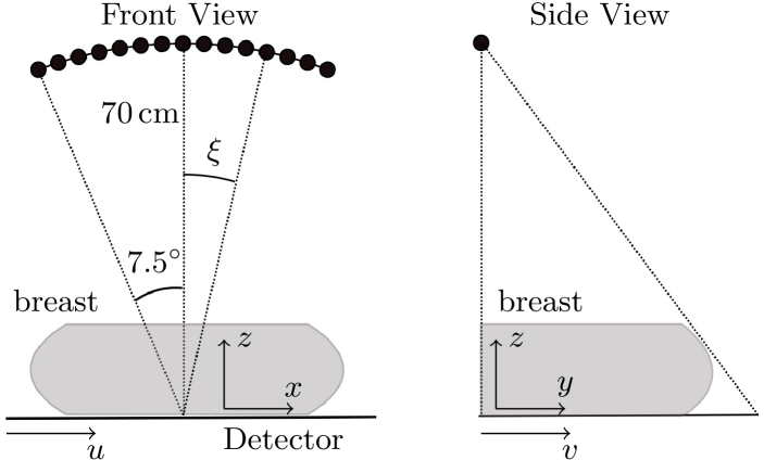
To explain the DBT data model and image reconstruction algorithms, we employ an approximate simplified geometric model for the DBT scan shown in Fig. 1. In this model, the detector is fixed; the X-ray source moves on a circular arc of 15 degrees, acquiring 15 projections in 1 degree increments; the center of the scanning arc lies on the detector; and the detector pixel size is 0.14 mm 0.14 mm. The various geometric parameters of the scan are also shown in the schematic in Fig. 1.
While the data model and image reconstruction theory is explained with the approximate stationary-detector model, the image reconstruction results are obtained with the precise scan geometry provided by the projection matrices.
II.2 DBT Data model
The X-ray transmission data are modeled with the Beer-Lambert law
| (1) |
where is the incident X-ray fluence; is the transmitted fluence for X-ray source angle and detector pixel location . The function represents the line integrals over the object function
| (2) |
where represents an energy-averaged map of the linear X-ray attenuation coefficient; the X-ray source position is ; and the unit vector indicates the direction of a ray originating from and incident on the detector at . Using the coordinate system shown in Fig. 1, the source position can be parameterized by
and the detector pixel locations by
where cm, the radius of the source trajectory, and cm, the length of the detector in the direction. The unit vector can then be written
The coordinates are shifted by with respect to the volume coordinates because the origin of the detector is taken to be at a corner, while the origin of the volume Cartesian coordinates coincides with the middle of the detector edge adjacent to the chest wall.
The noisy simulation data, which is generated for the results in Sec. III, use the Beer-Lambert model in Eq. (1) as a mean value for a Poisson distribution, where the noise level is specified by selecting the total number of photons, , incident at each detector bin. No correlation between detector bins is assumed.
II.3 DBT image reconstruction algorithms
For the results presented in Sec. III, four image reconstruction algorithms are compared. The first two are of the form of filtered back-projection (FBP). For background on application of FBP in CT, the reader is referred to Ref. Kak and Slaney, 1988, and for implementation of FBP specific to DBT, Ref. Mertelmeier, 2017. We also consider two common forms of penalized, least-squares optimization that we have already investigated in the context of signal detection in DBT Sanchez, Sidky, and Pan (2015); Rose et al. (2017).
For the FBP implementations, the general form of filtering considered involves only filtering along the detector -direction with the one-dimensional Fourier transform (FT) and inverse Fourier transform (IFT)
| (3) |
where integration over performs the FT; is the filter function; integration over performs the IFT; and is the filtered projection data.
The reconstructed volume is obtained from by back-projection,
| (4) |
where and are the coordinates on the detector pointed to by a ray originating at source position and passing through , i.e.
FBP - The filter for the first FBP algorithm is a ramp filter with a Hanning apodizing window
where is the cutoff frequency of the filter. The cutoff frequency is specified as a fraction of the detector’s Nyquist frequency
where is the detector bin size and is the fractional cutoff frequency. For the studies in Sec. III, we investigate the impact of on conspicuity of fiber-like signals.
mFBP - One strategy for designing analytic image reconstruction for tomosynthesis involves combining back-projection BP with ramp-filtered FBP. Such an admixture has been proposed for reduction of metal artifacts Gomi, Hirano, and Umeda (2009). A similar approach is to modify the FBP filter in such a way that its value at low spatial frequency is boosted with respect to the ramp Orman, Mertelmeier, and Haere (2006). For mFBP, short for modified FBP, we design a filter based on the latter idea. Our particular choice of filter function employs a shifted quadratic at low spatial frequency
where is specified in terms of a fraction of the detector’s Nyquist frequency. The filter used for mFBP is the product of the boosted filter and the Hanning apodization window for . For mFBP, is the only regularization parameter and is taken to be in the range .
At , is identical to for . The upper bound on the range is determined by the condition . This condition yields a flat response at low frequencies (the first derivative at is zero because the filter function is symmetric). At , becomes a low-pass filter and the corresponding mFBP reconstruction is approximately back-projection.
We point out that there is other work on deriving filters for FBP applied to tomosynthesis Stevens, Fahrig, and Pelc (2000); Kunze et al. (2007); Nielsen et al. (2012). Also, additional parameters such as a slice thickness filter or Hanning filter width can be beneficial for controlling the DBT image quality. Orman, Mertelmeier, and Haere (2006); Mertelmeier (2017) Our particular design results from empirical subjective assessment on volumes reconstructed with the Hologic geometry and the aim of having a single-parameter image reconstruction algorithm.
LSQI - We also investigate whether orientation-dependence of fiber-like signal conspicuity can be mitigated using iterative reconstruction algorithms. Such algorithms employ a discrete model, and for the present work we employ a voxel expansion to arrive at a discretized form of Eq. (2)
where is a vector of voxel coefficients; is a vector of the line-integral measurements; and is the system matrix generated by computing the projection of each of the voxel expansion elements. The dimensions of the voxels used here measure 0.140.14 mm2 in-plane and 1.3 mm in depth. In using and without parenthetical arguments, we are referring to the discrete digital data and voxel coefficients, respectively. With parenthetical arguments, and , we are referring to the continuous data function and volume, respectively.
We consider two forms of least-squares optimization. The first form of least-squares employs identity Tikhonov regularization (LSQI)
| (5) |
where is a normalized regularization parameter and is the maximum singular value of the system matrix . For more implementation details on LSQI for DBT, consult Ref. Rose et al., 2017.
In this particular formulation of LSQI, the parameter is dimensionless and the same value of will incur the same level of regularization no matter what length units are used in specifying . Some sense of the impact of can be deduced by deriving the small and large -value limits of the LSQI analytic solution.
Setting the gradient of the objective function in Eq. (5) to zero, and solving for yields a direct linear expression relating to the data
This expression is useful for interpreting the effect of the regularization parameter . The transpose of the projection matrix represents a form of discrete back-projection. The small limit tends to back-projection filtration (BPF)
where the discrete back-projection, , is followed by filtration in the form . Scaled appropriately, the large limit tends to back-projection Rose et al. (2017)
In practice, is obtained by iterative solution of Eq. (5) using the conjugate gradients algorithm.
LSQD - The second form of least-squares presented is more commonly used in tomographic applications than LSQI; namely, we consider least-squares with a quadratic roughness penalty Fessler (1994) (LSQD)
| (6) | ||||
where is a finite differencing matrix approximating the gradient operator. The scale factor serves to make the regularization parameter dimensionless.
The direct expression for the LSQD volume is
The small limit of this expression is the same as that of LSQI, a form of back-projection filtration. The scaled large limit, however, differs
The expression is a form of blurring, and as a result the large limit of LSQD is blurred back-projection.
Pyramidal image volume - The Hologic system reconstructs images onto a pyramidal volume to correct for the effects of magnification due to the extremely limited angular range. In terms of the continuous reconstructed volume, slices are displayed in the transformed coordinate system , where the transformed coordinates are related to the original Cartesian coordinates by
| (7) | |||
| (8) | |||
| (9) |
The reconstructed volume is represented in this new coordinate system by the function
Note that the transformed coordinates match the untransformed coordinates at the plane of the detector, i.e. . As increases, and adjust to counteract the magnification of the corresponding -plane. Results for all four investigated algorithms are presented in the transformed coordinates.
Background flattening - Raw reconstructions of the breast exhibit a low-frequency variation when reconstructing at larger regularization strengths. The effect is particularly strong near the skin line. This gray-level variation needs to be removed in order to display low-contrast tissue structures over extended areas of the breast. In the present work, we fit a low-order polynomial to the 2D slice images then divide the raw 2D slice image by this fitted polynomial.
II.4 Relative intensity metric for characterizing orientation-dependence of fiber-like signals
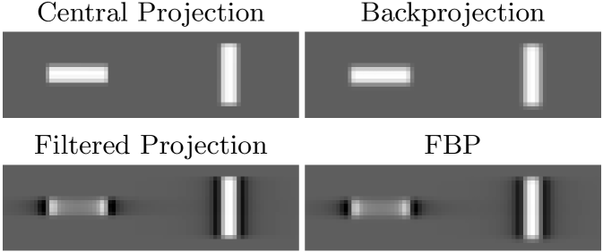
In order to provide background on fiber-like signal imaging in DBT and to motivate the relative intensity metric, we show tomosynthesis images of a rod aligned parallel and perpendicular to the direction of X-ray source travel (DXST) in Fig. 2. Shown are images for FBP using the ramp filtering
and no filtering
which corresponds to back-projection (BP). Because of the extremely limited angular range of the scan trajectory, the reconstructed slice images resemble closely the central filtered projection prior to back-projection.
In the FBP image of Fig. 2, the ramp filter causes two classic features of objects reconstructed in a tomosynthesis settingReiser and Glick (2014); Sechopoulos (2013): the ramp filter amplifies high frequency content in the -direction causing the edges perpendicular to the DXST to enhance, and it attenuates low frequency content in the -direction causing gray-level contrast to drop toward the middle of the signal. The impact of these FBP features differ greatly between the images of the two rods. For the rod parallel to the DXST, the edge-enhancement is minimal because the short edges are perpendicular to the DXST; furthermore, the gray-level contrast is low relative to the actual rod because the long-axis is parallel to the DXST. For the rod perpendicular to the DXST, the situation is reversed and the rod enhances well. These basic imaging properties are a direct result of the ramp filter, and this is seen in comparing the DBT slice images with the ramp filtered central projection in Fig. 2.
The BP image shown in Fig. 2 does not have either the edge-enhancement nor the drop in contrast in the signal interior. The central slice of the BP image appears to depict both rods faithfully. In comparing the FBP to BP images, the former clearly have a greater variation with in-plane orientation with respect to the DXST. In terms of conspicuity, BP will likely yield uniform results with respect to orientation. For FBP, conspicuity may vary greatly with orientation.
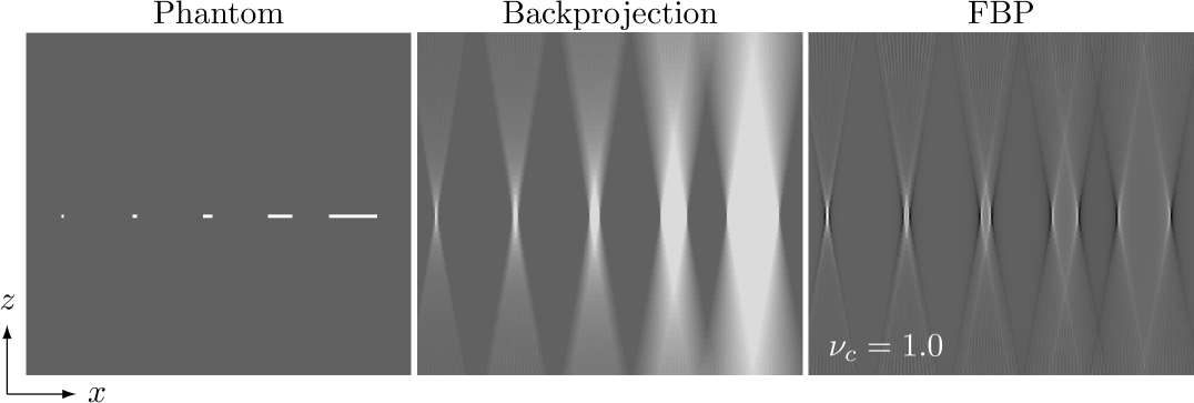
While the in-focus-plane images of Fig. 2 would seem to favor BP, there is, however, a penalty for the absence of filtering; namely the depth-blur of BP image reconstruction is significantly greater than that of FBP. The depth blur of reconstructed rod signals of different lengths is shown in Fig. 3 in a non-standard viewing plane. The images are shown for planes aligned along the DXST and perpendicular to the detector. The BP image strongly displays the classic size-dependent depth blur of DBT; the BP depth blur has a central diamond shaped region of nearly uniform gray values, and outside of this region the intensity slowly dissipates. The geometry of the central diamond region is determined by the -extent of the rod and the scanning angular range, which for the present configuration is 15∘. For FBP, the reconstructed rod images in the depth plane have quite different appearances from those of BP. The ends of the rod are highlighted, but for the longer rods the “BP diamond” is suppressed including the mid-line where the actual rod is located.
Results from the investigated image reconstruction algorithms can be interpreted as some combination of the two extreme cases of FBP and BP. There is a trade-off for fiber-like signals. For FBP-like algorithms, there is strong orientation-dependence of the conspicuity in the focus plane. For BP-like algorithms, there is pronounced depth blur for fibers parallel to the DXST. To quantify this trade-off we employ a relative intensity metric defined through noiseless simulation of rod-signals.

Orientation-dependent relative intensity
We define a relative intensity metric to characterize reconstructed rod signal orientation-dependence and depth blur. Different reconstruction algorithms can yield large variation in gray scale values yet have similar conspicuity of vessels, ducts, masses, and microcalcifications. The variations in reconstructed gray scale also make comparison with the test object non-trivial Rose et al. (2017). We characterize rod signal fidelity with a metric derived from the reconstruction of a rod test phantom shown in Fig. 4. The background tissue is removed and only the rods are used in generating noiseless projection data.
The relative intensity metric involves line-integration of the reconstructed rod volume, , along a line segment parallel with the axis of the rod object
| (10) |
where and label the endpoints of the rod central axis; is the location of ; is the in-plane deflection of the rod axis from the DXST; the unit vector points in the direction of from ; is the rod axis length; and is the depth separation from the rod axis. Note that results in integration along the rod axis. This rod intensity measure applies to any rod signal, not just those shown in Fig. 4. The only restriction imposed is that the rod axis must lie within a slice; i.e. .
For the relative intensity metric, the line integration is normalized to that of of and
| (11) |
This definition is motivated by the observation from Fig. 2, that when orientation dependence is observed, the gray-level contrast is highest for the rod. The relative intensity for the rods in the phantom is 1.0, because all the phantom rods are of the same length and gray level. Thus, any deviation from 1.0 directly reflects orientation-dependent intensity induced by the image reconstruction algorithm. Ideally, should be independent of , 1.0 for , and 0.0 for , where is the rod radius. Depth blur causes to be larger than 0.0 for . The relative intensity metric tracks orientation dependence and persistence to out-of-focus planes for reconstructed rod objects.
III Results
The studies in Sec. III.1 and III.2 employ simulated data and the relative intensity metric to illustrate how the orientation-dependence of fiber intensity depends on each algorithm’s single free parameter. Orientation-dependence of fiber conspicuity is presented with physical phantom data in Sec. III.3. The algorithm dependences of the physical phantom images are shown in Sec. III.4. Finally, the impact of algorithm dependence on a clinical DBT case is presented in terms of fiber-like signal conspicuity in Sec. III.5.
III.1 Orientation dependence of rod-signal intensity
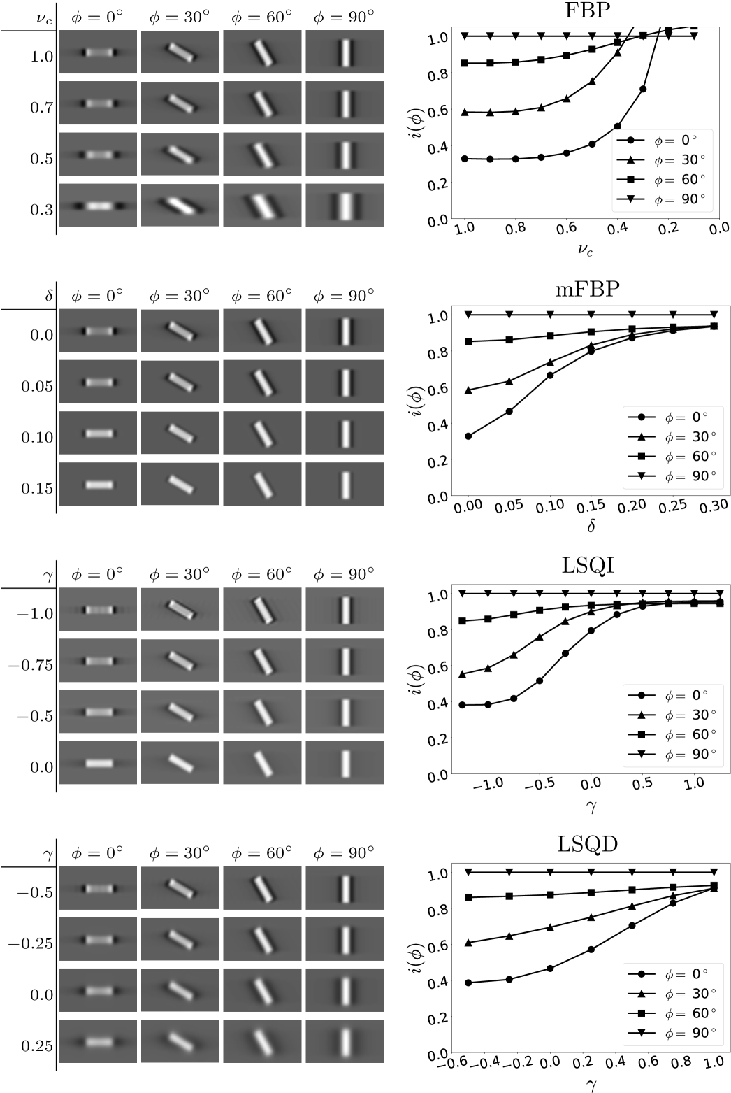
Zoomed in reconstructions of a subset of the rods are shown in Fig. 5 along with the orientation-dependent relative intensity metric. The shown images are in-plane and the relative intensity metric is abbreviated as with and mm. captures the trends in visual rod intensity relative to that of for the various algorithms and regularization strengths. Overall for each of the image reconstruction algorithms the deviation of from 1.0 is greatest for low regularization strength and small . Increasing regularization reduces the orientation-dependent rod intensity as the low rods show values of approaching 1.0.
The detailed behavior of each algorithm differs as each uses a different form of regularization. The FBP Hanning filter regularizes by smoothing the image in the -direction, and orientation-dependent intensity is mitigated with the smoothing filter width, defined by , comparable to the length of the rod signal. While the intensity of and rods appears similar at large regularization (low ), the distortion of the rod has strong dependence because of the directionality of the filter. The mFBP filter parameter interpolates between ramp-FBP and BP, and the rod signal intensity and shape become more uniform with increasing . The LSQI algorithm parameter ranges between similar extremes as mFBP and accordingly the resulting rod images are similar to mFBP. For LSQD, the low limit is similar to that of LSQI, but the large limit involves smoothing of a different form than the other three algorithms, which is reflected in the different appearance of the rod images.
III.2 The orientation-dependence of small rod conspicuity
The next set of simulation results illustrate how the intensity variation of fiber-like signals reconstructed from noiseless data translate to variation in signal conspicuity in the presence of noise. The simulated data are generated from projections with the complete test phantom illustrated in Fig. 4 that contains a uniform background block and 10 rod signals oriented in angular increments of over a range of to with respect to the -axis. Noise is modeled as an independent Poisson process in the transmission data with a mean incident intensity of photons per ray.
The central slice from each reconstructed volume is shown in Fig. 6. Assessing the shown images for rod conspicuity yields an overview of in-plane orientation-dependence and the impact of the various algorithms and forms of regularization. Starting with FBP in the upper left set of images, there is a clear orientation-dependence of the rod conspicuity for , the least regularized case. The rod conspicuity increases with increasing angle to the -axis, the DXST. Increasing regularization, by decreasing , visually seems to improve the conspicuity of the low-angle rods.
For each of the other three algorithms, mFBP, LSQI, and LSQD, at an overview level, we observe similar trends to that of FBP for rod conspicuity. For the least regularized phantom image, there is a strong orientation dependence with rod angle. Increasing regularization strength improves the conspicuity of the rod-signals nearly parallel to the DXST. These rod-conspicuity results are fairly consistent despite the obvious differences in other image quality characteristics, such as noise texture or blur.
III.3 Orientation-dependence of ACR-DM phantom fiber conspicuity
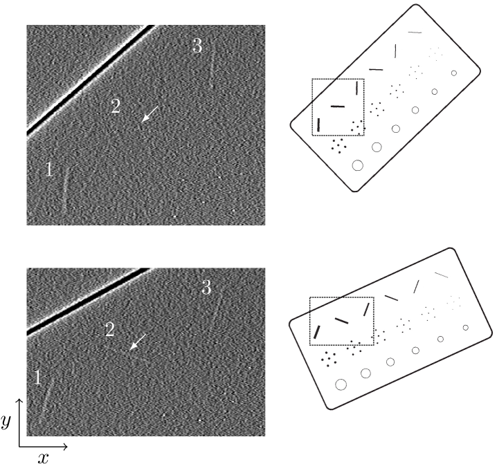

To demonstrate the in-plane anisotropy of fiber-like signals, we show FBP reconstructions () of the ACR-DM phantom at two orientations in Fig. 7. In Fig. 7 the DXST is from left to right, and in the top row the ACR-DM phantom is oriented at approximately a 40∘ angle from the DXST. Orienting the phantom in this way causes the odd-numbered fibers to line up nearly perpendicular to the DXST. The top-left panel image shows the first three fibers, and the striking feature is that the second fiber is invisible while fibers one and three are clearly seen. Even more striking is that the fibers are numbered in order of decreasing thickness, yet, fiber number three is seen and thicker fiber number two is not. The bottom-row illustrates the imaging properties of the same phantom when tilted 10∘ from the top-row orientation. This change in ACR-DM phantom orientation causes the second fiber to appear in the bottom-left panel image. The top-row image clearly displays how fiber-like signals enhance when oriented perpendicular to the DXST while those parallel do not; the bottom-row image hints at the strong dependence of fiber-like signal conspicuity for orientations close to the DXST.
III.4 Algorithm dependence of ACR phantom fiber conspicuity
We expand upon the results shown in Sec. III.3 for the ACR-DM phantom tilted at so that the fiber objects line up at and with respect to the DXST. The ACR-DM phantom data is reconstructed by the four considered algorithms at matched resolution with FBP. The regularization equivalence among the four reconstruction algorithms is established by matching the artifact spread function (ASF) Wu et al. (2004); Hu, Zhao, and Zhao (2008) of a simulated small point-like object: a sphere of 28.0 m diameter and attenuation coefficient of 9.29 cm-1, modeling a microcalcification.
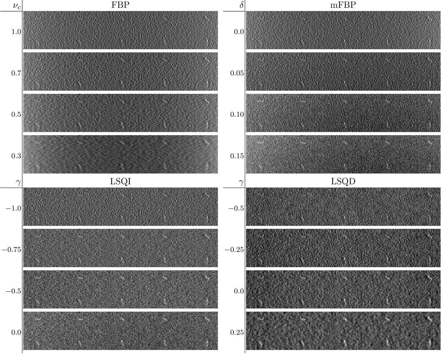
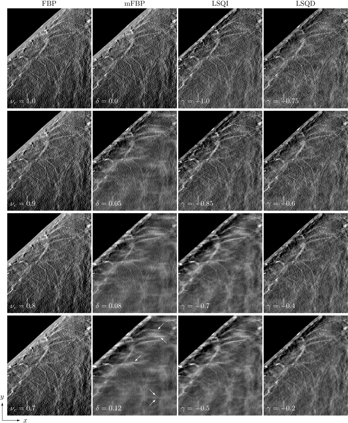
In Fig. 8, we show ACR-DM images for the 40∘ orientation so that fiber signals at 5∘ and 95∘ are presented. The 5∘ fiber is difficult to see; it is visible in three of the mFBP images, two of the LSQI images, and none of the LSQD and FBP images . We note that there are differences in the noise texture among the images from the various algorithms. In particular, that of LSQD is markedly different than that of the other three, and the differences in noise texture can impact the fiber conspicuity.
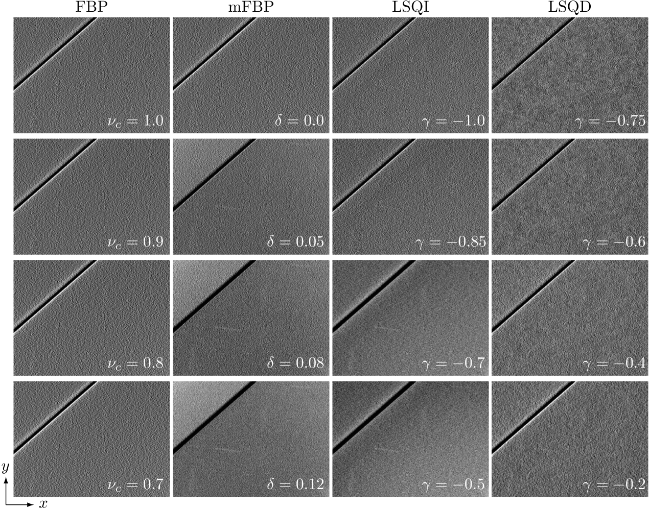
Fig. 9 is identical with Fig. 8 except that the shown images are from a slice 7.7 mm below the focus plane for the ACR-DM fibers. The shown plane is well below the fibers. The main point of viewing this out-of-focus plane is to observe the extent to which fiber signals bleed through, yielding a sense of the object-dependent blur. Most notable is the fact that the 5∘ fiber is still visible for the more regularized images of mFBP and LSQI. Thus, it appears that the improved conspicuity of the fiber for the regularized mFBP and LSQI in-focus images comes at a price; namely, this fiber persist strongly to out-of-focus planes.
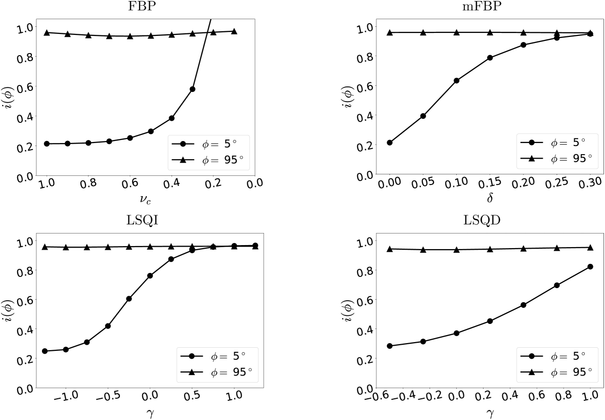
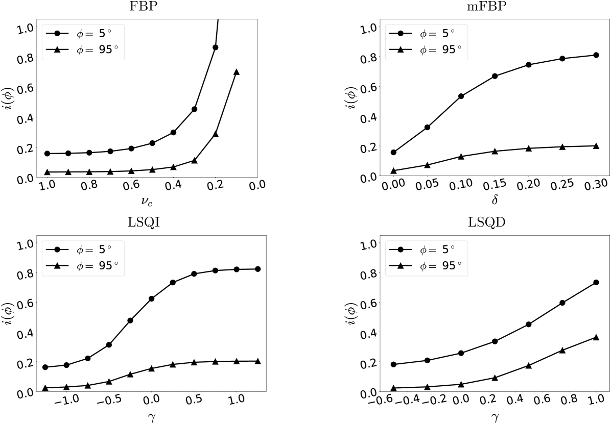
The relative intensity metric provides a means to interpret the fiber conspicuity in the DBT scanner images of the tilted ACR-DM phantom. For the present purpose, the metric is written to allow for -dependence and the rod length is set to mm to match the ACR phantom fiber length. The in-focus plane images in Fig. 8 correspond to the relative intensity plots shown in Fig. 10. Compared to the shorter rods of Fig. 5 the dependences in the relative intensity for the rods is more exaggerated. In particular, the rod signals nearly parallel to the DXST have a much lower relative intensity than their shorter counterparts. This agrees with the visual assessment of the fiber signals in Fig. 8, where the 5∘ fiber is difficult to see except when strong regularization is employed. The images in Fig. 9 shown for planes below the focus plane correspond to the curves plotted in Fig. 11. The relative intensity curves track the persistence of the small-angle ACR-DM fibers from Fig. 9 seen for regularized mFBP and LSQI. The corresponding relative intensity curves in Fig. 11 increase with greater regularization particularly for the low-angle rods reconstructed with mFBP and LSQI. This result demonstrates the trade-off between in-focus-plane orientation dependence of fiber conspicuity and depth blur of fibers nearly parallel to the DXST.
III.5 Fiber-like structure conspicuity algorithm dependence for a clinical DBT case
Up until the present section, we have focused on various aspects of the imaging of fiber-like structures embedded in uniform backgrounds. To investigate visualization of fiber-like signals in the presence of realistic background structure, we show an ROI from a clinical DBT case reconstructed by FBP, mFBP, LSQI, and LSQD. The chosen ROI has fibrous structures at different orientations so that some of the discussed trends in rod signal conspicuity can be illustrated.
In Fig. 12 an ROI from a clinical case is displayed in an arrangement similar to the ACR-DM images shown in Fig. 8; the same ROI is shown for FBP, mFBP, LSQI, and LSQD at the same regularization strengths used for the ACR-DM images. This particular ROI is chosen because of the presence of multiple fiber-like structures at various in-plane orientations; and the conspicuity of these structures can be compared among the algorithms and regularization strengths. In particular, we highlight a group of three nearly horizontal vessels that change in conspicuity dramatically depending on algorithm and regularization parameter setting. Their conspicuity varies in a manner consistent with the presented rod-signal simulations and ACR-DM phantom results.
The background texture in the patient images of Fig. 12 is seen to vary among the algorithms and parameter settings, and the differences are more obvious than what is seen in the ACR-DM images of Fig. 8. One aspect of the texture can be traced to imaging of fiber-like structures; the mFBP images show horizontal wisp artifacts for and to a slightly lesser degree the same wispiness is seen in LSQI for . These artifacts can be traced to vessels that are present at slices of different depths. For example, the indicated horizontal wisp in the mFBP image for can be traced to a vessel oriented parallel to the DXST in a plane that is 1.3 cm below the shown image. The horizontal wispiness is a direct result of the persistence of horizontal fiber-like structures from other slices at different depths.
IV Discussion and conclusion
The clinical DBT images demonstrate that orientation-dependent conspicuity of fiber-like signals can play a role in determining image reconstruction algorithm and regularization parameter settings. To help guide the design of DBT image reconstruction algorithms, a relative intensity metric is proposed. This metric quantifies the orientation-dependent intensity and depth blur of fiber-like objects. It is a summary metric that is a descriptive property of noiseless reconstructions of rod signals, and it is predictive of the gross behavior of conspicuity of fiber-like structures in the presence of noise.
The simulation trends agree well with visualization of the fibers in the ACR-DM phantom. The utility of the simulation metrics is that they allow for quantitative comparison between algorithms and regularization settings; visualization of physical phantom images is subjective and affected by the gray-level window settings and post-processing algorithms. The trends in rod signal imaging revealed by the simulation studies also help to explain features of imaging fiber-like structures in clinical DBT. In particular, it is observed that fiber-like structures that run parallel to the direction of X-ray source travel (DXST) can have their intensity suppressed relative to the similar in-plane structures that are oriented obliquely to the DXST. Regularization that involves admixture of back-projection can dramatically improve the conspicuity of fiber-like structures parallel to the DXST at the expense of incurring depth blur of the same structures.
The rod signal relative intensity metric is motivated in this work by a need to explain variations in fiber-like structure conspicuity. The natural extension of this idea is to develop model observers for detection of the rod signals Diaz et al. (2015); Rose et al. (2017, 2018). Even if such model observers are developed, the present relative intensity metric can still provide useful information. In particular, it can be directly applied to non-linear image reconstruction algorithm development for DBT Sidky et al. (2009); Zheng, Fessler, and Chan (2018); Garrett et al. (2018); Lu et al. (2010); Ertas et al. (2013); Das et al. (2011); Michielsen et al. (2013); Piccolomini and Morotti (2016).
However, care must be taken to properly tailor the test phantom to challenge the assumptions of the non-linear algorithm. For example, the uniform background may lead to an optimistic assessment of total-variation (TV) based algorithms that exploit gradient sparsity. In such a case it may be prudent to embed the rod signals in some form of structured background.
Finally, the DXST is seen to play a large role in imaging fiber-like structure; thus it may be interesting to investigate rod signal conspicuity with different X-ray source trajectories. For example, while strong orientation dependence of fiber-like signal conspicuity was observed in this work when reconstructing with low regularization settings, we would expect this effect to be less pronounced if X-ray projections were acquired over a larger angular span. A source trajectory was considered in this work, but there exist clinical tomosynthesis systems employing angular ranges up to . The variation in depth blur and orientation dependent conspicuity as the regularization strength is increased would appear differently for such systems. Crosstalk between slices would, in general, be expected to be less pronounced at all regularization strengths. We therefore emphasize that the particular results presented here concern the source trajectory.
In conclusion, we have investigated the impact of image reconstruction algorithm and associated parameter settings on imaging of fiber-like structures. For the shown algorithms at a low regularization setting, a strong orientation-dependence in the conspicuity of fiber-like signals is observed in simulation, physical phantom, and clinical data. In particular, fiber-like objects nearly parallel to the DXST show a drop in conspicuity. Increasing regularization strength mitigates this orientation dependence at the cost of increasing depth blur of these structures.
V Disclosure of Conflicts of Interest
The authors have received a research grant from Hologic, Inc.
VI Acknowledgements
The authors would like to thank Drs. Chris Ruth, Yiheng Zhang, and Chao Huang from Hologic for providing data and useful discussion. This work was supported in part by NIH R01 Grants Nos. CA182264, EB018102, EB026282 and NIH F31 Grant No. EB023076. The contents of this article are solely the responsibility of the authors and do not necessarily represent the official views of the National Institutes of Health.
References
- Sechopoulos (2013) I. Sechopoulos, “A review of breast tomosynthesis. Part II. Image reconstruction, processing and analysis, and advanced applications,” Med. Phys. 40, 14302 (2013).
- Zhou, Zhao, and Zhao (2007) J. Zhou, B. Zhao, and W. Zhao, “A computer simulation platform for the optimization of a breast tomosynthesis system,” Med. Phys. 34, 1098–1109 (2007).
- Hu, Zhao, and Zhao (2008) Y.-H. Hu, B. Zhao, and W. Zhao, “Image artifacts in digital breast tomosynthesis: Investigation of the effects of system geometry and reconstruction parameters using a linear system approach.” Med. Phys. 35, 5242–5252 (2008).
- Zhao et al. (2009) B. Zhao, J. Zhou, Y.-H. Hu, T. Mertelmeier, J. Ludwig, and W. Zhao, “Experimental validation of a three-dimensional linear system model for breast tomosynthesis,” Med. Phys. 1, 240–251 (2009).
- Chawla et al. (2009) A. S. Chawla, J. Y. Lo, J. A. Baker, and E. Samei, “Optimized image acquisition for breast tomosynthesis in projection and reconstruction space,” Med. Phys. 36, 4859–4869 (2009).
- Sechopoulos and Ghetti (2009) I. Sechopoulos and C. Ghetti, “Optimization of the acquisition geometry in digital tomosynthesis of the breast.” Med. Phys. 36, 1199–1207 (2009).
- Saunders et al. (2009) R. S. Saunders, E. Samei, J. Y. Lo, and J. A. Baker, “Can compression be reduced for breast tomosynthesis? Monte carlo study on mass and microcalcification conspicuity in tomosynthesis.” Radiology 251, 673–682 (2009).
- Park et al. (2010) S. Park, R. Jennings, H. Liu, A. Badano, and K. Myers, “A statistical, task-based evaluation method for three-dimensional x-ray breast imaging systems using variable-background phantoms.” Med. Phys. 37, 6253–6270 (2010).
- Reiser and Nishikawa (2010) I. Reiser and R. M. Nishikawa, “Task-based assessment of breast tomosynthesis: Effect of acquisition parameters and quantum noise.” Med. Phys. 37, 1591–600 (2010).
- Richard and Samei (2010) S. Richard and E. Samei, “Quantitative imaging in breast tomosynthesis and CT: Comparison of detection and estimation task performance.” Med. Phys. 37, 2627–2637 (2010).
- Gang et al. (2011) G. J. Gang, J. Lee, J. W. Stayman, D. J. Tward, W. Zbijewski, J. L. Prince, and J. H. Siewerdsen, “Analysis of Fourier-domain task-based detectability index in tomosynthesis and cone-beam CT in relation to human observer performance.” Med. Phys. 38, 1754–1768 (2011).
- Lu et al. (2011) Y. Lu, H.-P. Chan, J. Wei, M. Goodsitt, P. L. Carson, L. Hadjiiski, A. Schmitz, J. W. Eberhard, and B. E. H. Claus, “Image quality of microcalcifications in digital breast tomosynthesis: Effects of projection-view distributions,” Med. Phys. 38, 5703–5712 (2011).
- Young et al. (2013) S. Young, P. R. Bakic, K. J. Myers, R. J. Jennings, and S. Park, “A virtual trial framework for quantifying the detectability of masses in breast tomosynthesis projection data.” Med. Phys. 40, 051914 (2013).
- Tucker, Hill, and Zhou (2013) A. W. Tucker, C. Hill, and O. Zhou, “Dependency of image quality on system configuration parameters in a stationary digital breast tomosynthesis system,” Med. Phys. 40, 031917 (2013).
- Chan et al. (2014) H.-P. Chan, M. M. Goodsitt, M. A. Helvie, S. Zelakiewicz, A. Schmitz, M. Noroozian, C. Pramagul, M. A. Roubidoux, A. V. Nees, C. H. Neal, P. Carson, Y. Lu, L. Hadjiiski, and J. Wei, “Digital breast tomosynthesis: Observer performance of clustered microcalcification detection on breast phantom images acquired with an experimental system using variable scan angles, angular increments, and number of projection views,” Radiology 273, 675–685 (2014).
- Goodsitt et al. (2014) M. M. Goodsitt, H.-P. Chan, A. Schmitz, S. Zelakiewicz, S. Telang, L. Hadjiiski, K. Watcharotone, M. A. Helvie, N. Colleen, C. Paramagul, E. Christodoulou, S. C. Larson, and P. L. Carson, “Digital breast tomosynthesis: Studies of the effects of acquisition geometry on contrast-to-noise ratio and observer preference of low-contrast objects in breast phantom images,” Phys Med Biol. 59, 5883–5902 (2014).
- Wu et al. (2004) T. Wu, R. H. Moore, E. A. Rafferty, and D. B. Kopans, “A comparison of reconstruction algorithms for breast tomosynthesis.” Med. Phys. 31, 2636–2647 (2004).
- Mertelmeier et al. (2006) T. Mertelmeier, J. Orman, W. Haerer, and M. K. Dudam, “Optimizing filtered backprojection reconstruction for a breast tomosynthesis prototype device,” in Proc SPIE, Vol. 6142 (2006) pp. 131–142.
- Van de Sompel, Brady, and Boone (2011) D. Van de Sompel, S. M. Brady, and J. Boone, “Task-based performance analysis of FBP, SART and ML for digital breast tomosynthesis using signal CNR and Channelised Hotelling Observers,” Med. Image Anal. 15, 53–70 (2011).
- Zeng et al. (2015) R. Zeng, S. Park, P. Bakic, and K. J. Myers, “Evaluating the sensitivity of the optimization of acquisition geometry to the choice of reconstruction algorithm in digital breast tomosynthesis through a simulation study.” Phys. Med. Biol. 60, 1259–88 (2015).
- Sanchez, Sidky, and Pan (2015) A. A. Sanchez, E. Y. Sidky, and X. Pan, “Use of the Hotelling observer to optimize image reconstruction in digital breast tomosynthesis,” J. Med. Imaging 3, 011008 (2015).
- Rose et al. (2017) S. D. Rose, A. A. Sanchez, E. Y. Sidky, and X. Pan, “Investigating simulation-based metrics for characterizing linear iterative reconstruction in digital breast tomosynthesis,” Med. Phys. 44, 279–296 (2017).
- Maidment (2017) A. Maidment, “AAPM Medical Physics Tutorial Session 1: Digital Breast Tomosynthesis,” (Presented at the 2017 meeting of the Radiological Society of North America, 2017).
- Li, Da, and Liu (2010) X. Li, Z. Da, and B. Liu, “A generic geometric calibration method for tomographic imaging systems with flat-panel detectors – A detailed implementation guide.” Med. Phys. 37, 3844–3854 (2010).
- Kak and Slaney (1988) A. C. Kak and M. Slaney, Principles of Computerized Tomographic Imaging (IEEE Press, Piscataway, NJ, 1988).
- Mertelmeier (2017) T. Mertelmeier, “Filtered backprojection-based methods for tomosynthesis image reconstruction,” in Tomosynthesis Imaging, edited by I. Reiser and S. Glick (Taylor and Francis, 2017) Chap. 7, pp. 101–106.
- Gomi, Hirano, and Umeda (2009) T. Gomi, H. Hirano, and T. Umeda, “Computerized medical imaging and graphics evaluation of the X-ray digital linear tomosynthesis reconstruction processing method for metal artifact reduction,” Comput. Med. Imaging Graph. 33, 267–274 (2009).
- Orman, Mertelmeier, and Haere (2006) J. Orman, T. Mertelmeier, and W. Haere, “Adaptation of image quality using various filter setups in the filtered backprojection approach for digital breast tomosynthesis,” in Proc. 8th Int. Work. Digit. Mammogr. (2006) pp. 175–182.
- Stevens, Fahrig, and Pelc (2000) G. M. Stevens, R. Fahrig, and N. J. Pelc, “Filtered backprojection for modifying the impulse response of circular tomosynthesis,” Med. Phys. 28, 372–380 (2000).
- Kunze et al. (2007) H. Kunze, W. Härer, J. Orman, T. Mertelmeier, and K. Stierstorfer, “Filter Determination for Tomosynthesis Aided by Iterative Reconstruction Techniques,” in Proc. 9th Int. Meet. Fully Three-Dimensional Image Reconstr. Radiol. Nucl. Med. (2007) pp. 309–312.
- Nielsen et al. (2012) T. Nielsen, S. Hitziger, M. Grass, and A. Iske, “Filter calculation for X-ray tomosynthesis reconstruction,” Phys. Med. Biol. 57, 3915–3930 (2012).
- Fessler (1994) J. A. Fessler, “Penalized weighted least-squares image reconstruction for positron emission tomography,” IEEE Trans. Med. Imaging 13, 290–300 (1994).
- Reiser and Glick (2014) I. Reiser and S. J. Glick, Tomosynthesis Imaging (Taylor & Francis, 2014).
- Diaz et al. (2015) I. Diaz, C. K. Abbey, P. A. S. Timberg, M. P. Eckstein, F. R. Verdun, C. Castella, and F. O. Bochud, “Derivation of an observer model adapted to irregular signals based on convolution channels,” IEEE Trans. Med. Imaging 34, 1428–1435 (2015).
- Rose et al. (2018) S. Rose, J. Roth, C. Zimmerman, I. Reiser, E. Y. Sidky, and X. Pan, “Parameter selection with the Hotelling Observer in linear iterative image reconstruction for breast tomosynthesis,” in Proc. SPIE (in press 2018).
- Sidky et al. (2009) E. Y. Sidky, X. Pan, I. S. Reiser, R. M. Nishikawa, R. H. Moore, and D. B. Kopans, “Enhanced imaging of microcalcifications in digital breast tomosynthesis through improved image-reconstruction algorithms,” Med. Phys. 36, 4920–4932 (2009).
- Zheng, Fessler, and Chan (2018) J. Zheng, J. A. Fessler, and H.-P. Chan, “Detector blur and correlated noise modeling for digital breast tomosynthesis reconstruction,” IEEE Trans. Med. Imaging 37, 116–127 (2018).
- Garrett et al. (2018) J. W. Garrett, Y. Li, K. Li, and G. Chen, “Reduced anatomical clutter in digital breast tomosynthesis with statistical iterative reconstruction,” Med. Phys. 45, 2009–2022 (2018), https://aapm.onlinelibrary.wiley.com/doi/pdf/10.1002/mp.12864 .
- Lu et al. (2010) Y. Lu, H.-P. Chan, J. Wei, and L. M. Hadjiiski, “Selective-diffusion regularization for enhancement of microcalcifications in digital breast tomosynthesis reconstruction,” Med. Phys. 37, 6003–6014 (2010).
- Ertas et al. (2013) M. Ertas, I. Yildirim, M. Kamasak, and A. Akan, “Digital breast tomosynthesis image reconstruction using 2D and 3D total variation minimization,” Biomed. Eng. Online 12, 1–12 (2013).
- Das et al. (2011) M. Das, H. C. Gifford, J. M. O. Connor, and S. J. Glick, “Penalized maximum likelihood reconstruction for improved microcalcification detection in breast tomosynthesis,” IEEE Trans. Med. Imaging 30, 904–914 (2011).
- Michielsen et al. (2013) K. Michielsen, K. V. Slambrouck, A. Jerebko, and J. Nuyts, “Patchwork reconstruction with resolution modeling for digital breast tomosynthesis,” Med. Phys. 40, art. no. 031105 (2013).
- Piccolomini and Morotti (2016) E. L. Piccolomini and E. Morotti, “A fast total variation-based iterative algorithm for digital breast tomosynthesis image reconstruction,” Journal of Algorithms and Computational Technology 10, 277–289 (2016).