Impact angle control of interplanetary shock geoeffectiveness
Abstract
We use OpenGGCM global MHD simulations to study the nightside magnetospheric, magnetotail, and ionospheric responses to interplanetary (IP) fast forward shocks. Three cases are presented in this study: two inclined oblique shocks, hereafter IOS-1 and IOS-2, where the latter has a Mach number twice stronger than the former. Both shocks have impact angles of 30o in relation to the Sun-Earth line. Lastly, we choose a frontal perpendicular shock, FPS, whose shock normal is along the Sun-Earth line, with the same Mach number as IOS-1. We find that, in the IOS-1 case, due to the north-south asymmetry, the magnetotail is deflected southward, leading to a mild compression. The geomagnetic activity observed in the nightside ionosphere is then weak. On the other hand, in the head-on case, the FPS compresses the magnetotail from both sides symmetrically. This compression triggers a substorm allowing a larger amount of stored energy in the magnetotail to be released to the nightside ionosphere, resulting in stronger geomagnetic activity. By comparing IOS-2 and FPS, we find that, despite the IOS-2 having a larger Mach number, the FPS leads to a larger geomagnetic response in the nightside ionosphere. As a result, we conclude that IP shocks with similar upstream conditions, such as magnetic field, speed, density, and Mach number, can have different geoeffectiveness, depending on their shock normal orientation.
Gindraft=false \authorrunningheadOLIVEIRA AND RAEDER \titlerunningheadSYMMETRY OF IP SHOCKS \authoraddrCorresponding author: Denny Oliveira, EOS Space Science Center, University of New Hampshire, Durham, NH USA. (dmz224@wildcats.unh.edu)
1 Introduction
Interplanetary (IP) shocks are ubiquitous features of the solar wind (Burlaga, 1971). As they encounter Earth they interact with the magnetosphere, causing disturbances that can be seen everywhere in the magnetosphere. Because the disturbances alter the magnetospheric current systems, the ionosphere is also affected, and the magnetic field on the ground is perturbed as well. The most dramatic shock-induced ground perturbations are the storm sudden commencements (SSCs), which are driven by a strong IP shock preceding a geomagnetic storm driven by coronal mass ejections (CMEs).
The interaction of IP shocks with the Earth’s magnetosphere is both complex and important. For example, the shock-shock interactions such as between an IP shock and the Earth’s bow shock may occur in many contexts, for example, in the heliosphere and in astrophysical systems. Such remote interactions are difficult to observe, but can be readily observed with in-situ measurements in the magnetosphere. On the other hand, strong IP shock impacts on the magnetosphere have substantial space weather effects, for example, they produce geomagnetically induced currents (GICs), which can impact power grids (Bolduc, 2002; Kappenman, 2010), and they can energize particles in the inner magnetosphere (Hudson et al., 1997; Zong et al., 2009). Echer et al. (2004) reported that 22% of all interplanetary shocks are intensely geoeffective while 35% are moderately geoeffective. Thus, the study of IP shock impacts is of fundamental and also of practical importance.
At 1 AU (astronomical unit) IP shocks are almost exclusively fast shocks. Slow shocks may exist at closer distances to the Sun, but they are subject to Landau damping (Richter et al., 1985). IP shocks may further be classified as propagating away from the Sun, i.e., forward shocks, or as propagating towards the Sun, i.e., so-called reverse shocks. Since the solar wind speed is almost always supermagnetosonic, a reverse shock will still propagate away from the Sun in the Earth’s frame. IP shocks may then be further classified by their strength, i.e., their Mach number in the solar wind reference frame, their orientation, and by the orientation of their upstream field with respect to the shock normal. The compression ratio, i.e., the ratio of downstream to upstream plasma density, is an alternative measure for the shock strength, which is often more convenient to use than the Mach number. Assuming a (specific heat ratio) of 5/3 appropriate for a monoatomic gas, the compression ratio must lie between 1 and 4 (Priest, 1981). IP shocks are typically weak (compared to planetary bow shocks) with a compression ratio between 1.2 and 2 (Berdichevsky et al., 2000). The Rankine-Hugoniot relations provide the jump conditions between the upstream and downstream plasma parameters in the MHD context (Jeffrey and Taniuti, 1964; Priest, 1981; Parks, 2004). Thus, given the upstream plasma and field parameters, as well as the shock normal, the downstream parameters can easily be calculated. The inverse calculation, i.e., determining the shock speed and orientation from measured upstream and downstream values, is generally a much more difficult problem, because the critical parameters that cannot be measured directly, such as the shock normal, depend in a very sensitive manner on the upstream and downstream plasma and field measurements. Near 1 AU, IP shocks can generally be assumed to be planar structures on the scale size of the Earth’s magnetosphere. For example, Russell et al. (1983) found the assumption of planarity consistent with measurements from four widely spaced solar wind monitors. Also using the assumption of shock planarity, Russell et al. (2000) estimated the shock normal orientation of a large IP shock with accuracy by comparing results of different IP shock normal determination methods.
The shock normal vector determines how the shock propagates through the heliosphere. Normals of most IP shocks generated by CMEs at 1 AU are concentrated near the Sun-Earth line (Richter et al., 1985). However, shocks driven by corotating interaction regions (CIRs), as a result of the slow solar wind compression by a fast stream, have normals inclined in relation to the Sun-Earth line (see, e.g., Siscoe, 1976; Pizzo, 1991, and references therein). For CIR-driven shocks, the normal angles in the azimuthal direction in relation to the solar coordinate system are generally equal or larger than the inclination angle (Siscoe, 1976; Pizzo, 1991).
Here, we are primarily concerned with the effect that the orientation of an IP shock has on its geoeffectiveness. Similar studies have been done in the past, but none have addressed the parameter space that we are concerned with. For example, Jurac et al. (2002) analyzed more than 100 IP shocks in terms of the angle between the shock normal and the upstream interplanetary magnetic field (IMF), also called obliquity. They found that there is about a 40% chance for an IP shock to be followed by an intense magnetic storm when the obliquity is 90o. These shocks are more likely to result in an intense storm than shocks whose normal are oblique to the IMF direction. Takeuchi et al. (2002) showed that the shock orientation plays an important role in controlling the rise time duration of an SSC, such that the rise time is longer in the case of larger impact angles. The unusual SSC rise time observed, 30 minutes, was explained by a gradual compression observed in the magnetosphere due to the fact that the shock normal had to be largely inclined to the dusk-ward direction. The interaction of IP shocks inclined in relation to the Sun-Earth line with the bow shock was also investigated by Grib and Pushkar (2006). They solved the Rankine-Hugoniot conditions numerically for different shock inclinations and one of their most important results was that, for shock normal inclinations between 60o and -60o, the density changed from dusk to dawn in the bow shock in the case where the discontinuity was a fast forward shock (FFS). Using ACE and Wind satellite data from 1995 to 2004, Wang et al. (2006) reported that, in a survey of nearly 300 FFSs, 75% of them were followed by SSCs observed on the ground. They also found that the shock impact angle plays an important role in determining the SSC rise time, as previously suggested by Takeuchi et al. (2002). When the shock speed (shock strength) was fixed, the more parallel the shock normal with the x-line, the smaller the rise time. The same occurred when they fixed the shock inclination and changed the shock speed. The faster the shock, the shorter the SSC rise time.
Several authors have studied the interaction of IP shocks with the Earth’s magnetosphere in the context of numerical MHD simulations. However, almost always the IP shock hit the bow shock at the subsolar point head-on. For instance, Ridley et al. (2006) simulated an extreme IP shock driven by a Carrington-like CME (Manchester et al., 2006) that pushed the magnetopause toward the Earth to the limit of their code boundary, which was at 2 RE. They also observed a secondary shock wave reflected back by the magnetopause that encountered the bow shock that was moving inward. Then the combined motion propagated down the flanks of the magnetosphere. Similar bow shock Earth-ward motion was observed by S̆afránková et al. (2007) in their numerical simulation for a much weaker IP shock as well. The interaction of IP shocks with the Earth’s magnetosphere can also lead to generation of two ionospheric current systems (Ridley et al., 2006; Guo and Hu, 2007; Samsonov et al., 2010). The appearance of an anomalous region I current, which flowed oppositely to the region I current, followed by a frontal IP shock impact with no IMF was found by Guo and Hu (2007). This anomalous region I current formed at noon, developed and then moved toward the evening side until it vanished. Such a response depends on the strength of the IP shock. In other MHD simulations concerning the magnetosheath, three new discontinuities appeared downstream from the bow shock in addition to the FFS: a forward slow expansion wave, a contact discontinuity, and a reverse slow shock (Koval et al., 2006; Samsonov et al., 2006, 2007). Samsonov et al. (2010) simulated the interaction of an IP shock with the magnetosphere in an artificial case with a northward IMF. The IP shock normal was aligned with the Sun-Earth line. They observed an intensification of two ionospheric current systems (similar to the preliminary and main impulse currents) that coincided in time with the intensification of two corresponding magnetospheric dynamos.
Guo et al. (2005) performed a global numerical MHD simulation with different shock normal orientations to study the interaction of IP shocks with the Earth’s magnetosphere. They simulated two different cases with a Parker-spiral IMF orientation with no component. In their first case, the shock normal was parallel to the Sun-Earth line, and in their second case the shock normal was oblique to this line with an angle of 60o. They found that the inclined shock normal led to a longer evolution time of the system. Although both systems evolved from the same initial conditions in their numerical simulations, as can be seen in their Figure 4, they did not find any significant difference in the final quasi-steady state of the systems. Similar results were also found by Wang et al. (2005). More recently, similar results have been found by Samsonov (2011) as well. He presented a solution and analysis of the problem of an inclined IP shock incident on and propagating through the Earth’s magnetosheath. He showed that inclined IP shocks with normals in the equatorial plane result in a dawn-dusk asymmetry in the magnetosheath and predicted that this effect should be present in observations of sudden impulse inside the magnetosphere and on the ground.
Here, we show that the IP shock normal orientation is a critical parameter determining the geoeffectiveness of IP shocks. Preliminary results of this work were presented by Oliveira and Raeder (2013). IP shocks that have their normal aligned with the Sun-Earth line have the largest geoeffectiveness, because they compress the magnetosphere from all sides at the same time. By contrast, if the shock normal makes a large angle with the Sun-Earth line in the x-z plane in GSE (Geocentric Solar Ecliptic) coordinate system, the north-south asymmetry of the impact pushes the plasma sheet either to the north or to the south without much compression, which leads to a much weaker response.
In the following, we describe the model in section 2, in section 3 we present our results, and in section 4 we summarize and discuss our results.
2 OpenGGCM Model
We use the Open Geospace General Circulation Model (OpenGGCM) to study the impact of IP shocks on the magnetosphere. The OpenGGCM is a global coupled model of the Earth’s magnetosphere, ionosphere, and thermosphere. It is available at the Community Coordinated Modeling Center (ccmc.nasa.gov) as a community model for model runs on demand (Rastätter et al., 2013; Pulkkinen et al., 2011, 2013). The magnetosphere part solves the MHD equations as an initial-boundary-value problem. The MHD equations are solved to within 3 RE of Earth. The region within 3 RE is treated as a magnetosphere-ionosphere (MI) coupling region (Oliveira, 2014) where physical processes that couple the magnetosphere to the ionosphere-thermosphere system are parameterized using simple models and relationships. The ionosphere-thermosphere system is modeled using the NOAA CTIM (Coupled Thermosphere Ionosphere Model Fuller-Rowell et al. (1996); Raeder et al. (2001a)). The OpenGGCM has been described with some detail in the literature (see, e.g. Raeder et al., 2001b; Raeder, 2003; Raeder et al., 2008); we thus refer the reader to these papers. The OpenGGCM has been used for numerous studies, including studies of substorms (Raeder et al., 2001b; Ge et al., 2011; Gilson et al., 2012; Raeder et al., 2013), storms (Raeder et al., 2001a; Raeder and Lu, 2005; Rastätter et al., 2013; Pulkkinen et al., 2013), and, most relevant for this study, for the study of IP shock impacts (Shi et al., 2013).
3 Shock Impacts
3.1 Simulation setup
We use exclusively GSE coordinates in our simulation input data. The numerical box extends from the Earth 30 RE in the Sun-ward direction, and 300 RE down the tail. In the directions perpendicular to the Sun-Earth line, i.e., in the y and z directions, the numerical box extends to 50 RE. The numerical grid is non-equidistant Cartesian and is divided into 610256256 grid cells, such that the highest resolution is closest to Earth. Specifically, the grid resolution is 0.15 RE within a distance of 10 RE radially from the Earth. The inner boundary, where the magnetosphere variables connect via field-line mapping to the ionosphere is located at 3 RE.
In this paper we only consider IP shocks for which the shock normal lies in the GSE x-z plane. Furthermore, we assume that the IMF also has no GSE y-component. Thus, the shock geometry relative to the Earth and to the IMF depends exclusively on two angles. First, depending on the shock normal relative to the upstream (relative to the shock) magnetic field direction, a shock can be classified as perpendicular, oblique, or parallel (Burlaga, 1971; Tsurutani et al., 2011). As is often found in the literature (Burlaga, 1971; Tsurutani et al., 2011), when , the shock is classified as almost parallel. In the cases in which , the shock is said to be oblique. Finally, when , the shock is classified as almost perpendicular. In particular for this paper, the shock is named perpendicular when = 90o. Second, in relation to the Earth’s system of reference, the shock normal is decomposed in terms of two angles: the angle between the shock normal and the Sun-Earth line, and the angle in the x-y plane that completes the set, following the notation of Viñas and Scudder (1986). For our simulations presented here, is always 90o. We also assume average solar wind conditions, with a particle number density of 5 cm-3, thermal plasma pressure of 20 pPa, magnetic field magnitude of 7 nT, and background speed of = (-400,0,0) km/s in all cases upstream of the IP shocks. We specify the shock strength by its compression ratio. As reported by Echer et al. (2003), most shocks near Earth have a compression ratio of the order of 2 during solar maximum. Here, we then choose a compression ratio value of 1.5 in order to have a mild shock. The MHD code input is set as follows. We transform the upstream initial conditions into the shock frame, calculate the downstream parameters, and subsequently transform them back to the Earth’s system of reference. We ran simulations of different FFSs with different shock normal orientations, obliquities, shock speeds, Mach numbers, and IMF pointing either northward or southward. For brevity, we select three FFSs with different shock normal orientations and Mach numbers to discuss in detail. In the first case, the IP shock has its normal inclined with an angle of 30o with the GSE x-axis toward the south, =51o, shock speed = 380 km/s, and Mach number of 3.7, i.e., an inclined oblique shock, hereafter IOS-1. The second case corresponds to an FFS, also inclined and oblique here called IOS-2, with = 30o, = 45o, = 650 km/s, and Mach number of 7.4. In the last case the shock normal has = 0o and was perpendicular to the IMF, i.e., a frontal perpendicular shock (FPS), with = 650 km/s, and Mach number of 3.7. These shock speeds are consistent with the observations reported by Berdichevsky et al. (2000), where most FFSs have speeds in the range 50-200 km/s in the shock frame of reference. Tables 1,2, and 3 show the upstream (1) and downstream (2) and other important parameters for the three FFSs. The first and second shocks impact the magnetosphere (first contact with the magnetopause) at t = 16.45 minutes, and the FPS reaches the subsolar magnetopause at t=18.28 minutes. We also simulated shocks with northward IMF and otherwise identical solar wind conditions. We found that the results were similar to the southward cases, but with weaker magnetosphere response, with the exception that transient northward Bz (NBZ) currents occurred within a few seconds after the shock impact when it was frontal. This effect was already reported by Samsonov et al. (2010). We will thus focus on the case of southward IMF.
| IOS-1, = 380 km/s, M = 3.7 | ||||||
|---|---|---|---|---|---|---|
| = 51o, = 30o | ||||||
| upstream | -1.83 | -6.83 | -400.00 | 0.00 | 20.0 | 5.0 |
| downstream | -0.52 | -9.09 | -434.15 | -17.65 | 67.45 | 7.5 |
aB in nT, v in km/s, P in pPa, and n in particles/cm3.
| IOS-2, = 650 km/s, M = 7.4 | ||||||
|---|---|---|---|---|---|---|
| = 45o, = 30o | ||||||
| upstream | -1.83 | -6.83 | -400.00 | 0.00 | 20.0 | 5.0 |
| downstream | -0.52 | -9.09 | -461.53 | -28.61 | 109.74 | 7.5 |
| FPS, = 650 km/s, M = 3.7 | ||||||
|---|---|---|---|---|---|---|
| = 90o, = 0o | ||||||
| upstream | 0.00 | -7.07 | -400.00 | 0.00 | 20.0 | 5.0 |
| downstream | 0.00 | -10.61 | -483.33 | 0.00 | 191.37 | 7.5 |
3.2 Results
As the IP shock impacts the magnetopause, it launches waves into the magnetosphere. The phase speed of these waves (both Alfvén and magnetosonic waves) is generally much larger in the magnetosphere than in the solar wind and the magnetosheath. Therefore, the amplitude of the waves diminishes in the magnetosphere, because the waves are partially reflected and also because of the higher phase speed the wave energy spreads out more quickly. In order to visualize such waves, we therefore subtract consecutive time instances from each other to remove the background as much as possible. This essentially amounts to taking the time derivative. Thus, in the plots shown below, for any quantity , we show the difference , where is chosen to be 30 seconds. Figure 1 shows the time evolution of the total magnetic field changes (B), in nT, in the noon-midnight meridian plane. The left column shows the IOS-1 case, the middle column shows the IOS-2 case, and the right column shows the FPS case. Each row shows different time, and the time difference between rows is three minutes. The red color in the color bar shows an increasing magnetic field , and the blue color indicates where decreases. The color bar range is 2 nT. In all columns, the first plots show the instant right after the FFSs crosses the bow shock.
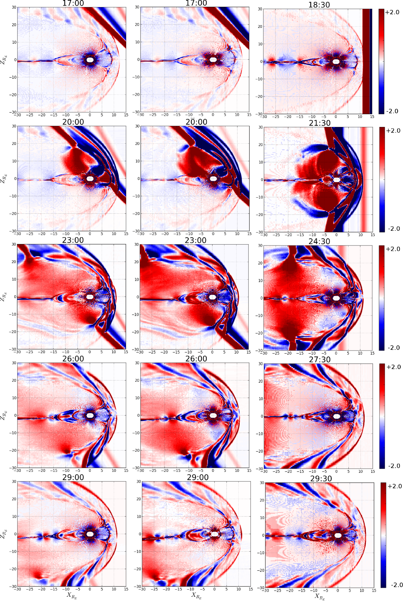
In Figure 1 the shock fronts appear much broader than they really are. First, by taking differences 30 seconds apart, the shock propagates 2-3 RE across the grid during that time, thus the shock will appear at least that wide. Second, because of numerical diffusion, the shocks have a foot or ramp on either side of the shock front. Normally, this would be hardly visible in a color-coded plot. However, because we take the differences and clamp the color bar at low values, these numerical artifacts become emphasized and make the shock appear much wider than it really is. In the simulation, the shocks are resolved to within 2-3 cells, i.e., to less than 0.5 RE within 10 RE from the x-axis.
As soon as the shock impacts the magnetopause, it launches Alfvén waves and magnetosonic waves into the magnetosphere. Because the wave speeds are much higher in the magnetosphere, these waves race ahead of the IP shock in the magnetosheath. The second row shows for both cases the time just after the IP shock has impacted the magnetopause. In the IOS-1 and IOS-2 cases, the first contact between the shock and the magnetopause occurs just past the northern cusp. The induced wave propagates through the northern lobe and reaches the plasma sheet in the nightside from the north. At this time, the IP shock has not yet impacted the southern hemisphere, and consequently there is no corresponding wave in the southern hemisphere yet.
The FPS case (second row, right panel) is distinctively different. The impacts on the northern and southern lobes occur simultaneously, and symmetric waves are launched from both the northern and southern magnetopause into the magnetosphere. These waves converge on the tail plasma sheet and cause a more significant compression of the plasma sheet.
As time progresses, these waves propagate further tail-ward. In the asymmetric cases, the waves from the southern hemisphere reach the near-Earth plasma sheet approximately 3 minutes after the waves from the northern hemisphere. As a result of such asymmetric impact, there is much less compression of the plasma sheet. Instead, the entire plasma sheet is bent southward. This is best visible at the later times (fourth and fifth row), where the deflection at x=-30 RE is as much as 3 RE in the IOS-1 case and 4 RE in the IOS-2 case. By contrast, in the symmetric case there is no such deflection, but instead a transient compression of the plasma sheet.
After the IP shock has passed (bottom row), the magnetosphere state seems to be very similar for the three cases. However, the particular display only shows differences to highlight transients and thus provides little information abut the state.
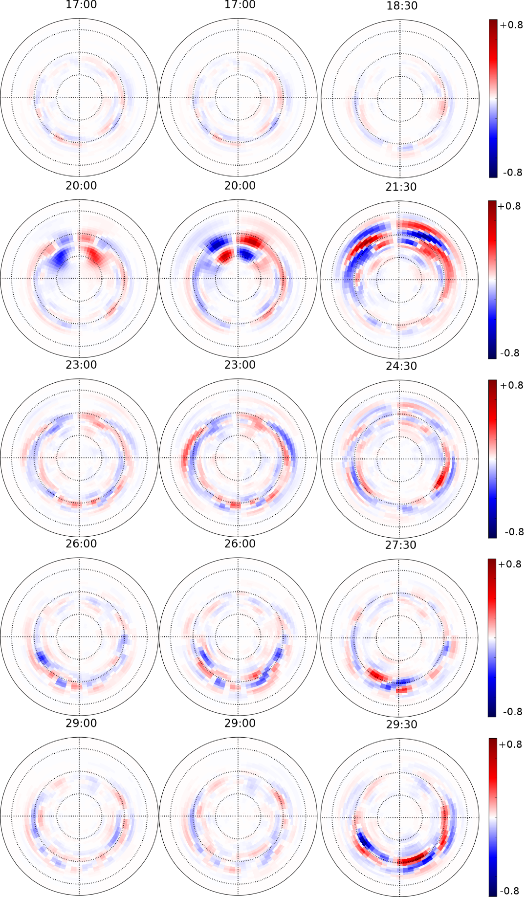
In order to examine the effects of the IP shocks on geomagnetic activity, we examine relevant ionospheric quantities. Figure 2 shows the time differences of the field-aligned current density (FAC, in A/m2) in the northern hemisphere polar cap, displayed in the same way as the magnetic field evolution of Figure 1. The times in Figure 2 correspond to the times shown in Figure 1, i.e., a time range of 12 minutes, plotted in three minute increments. The range in the color bar is 0.8 A/m2, and regions in red indicate a positive change in FAC, while regions in blue indicate a negative change in FACs. The dashed circles represent the magnetic latitude in 10 degree increments from 55o to the pole. Left, middle, and right columns represent the results for the IOS-1, IOS-2, and FPS cases, respectively. In all cases, in the first plot, the ionosphere is steady because the FFSs have not yet impacted the magnetopause. Also, in the three situations, the first FAC changes are seen about three minutes after the shock impact, as can be seen at t = 20:00 minutes for the inclined cases and t = 21:30 minutes for the FPS case. In the two IOS cases, the FAC changes are mostly in the vicinity of the cusp, whereas the FFS causes a broader signature that encompasses the entire dayside auroral region. The changes in the IOS-1 and IOS-2 cases are very similar geometrically, with the only difference that the IOS-2 response is slightly stronger than the IOS-1 response.
As time evolves, with the exception of the first minutes after the shock impact, the FAC signature diminishes in all cases, as can be seen in the middle row. Subsequently, activity in the nightside develops for the three cases. However, in the FPS case, the ionosphere response is much stronger. At t = 24:30 minutes, the enhancement of FACs is most evident on the nightside of the ionosphere between = 70o and = 65o, and between 0300 MLT and 0600 MLT. At t = 27:30 minutes and t = 29:30 minutes, FACs are enhanced close to midnight local time, which is a typical substorm signature (Akasofu, 1964; McPherron, 1991). The last row of Figure 2 shows the strongest nightside FAC variations occurring for the FPS case at t = 29:30 minutes, covering almost all the nightside ionosphere for between 70o and 65o. We attribute this activity due to substorm activity that was triggered by the converging waves in the plasma sheet.
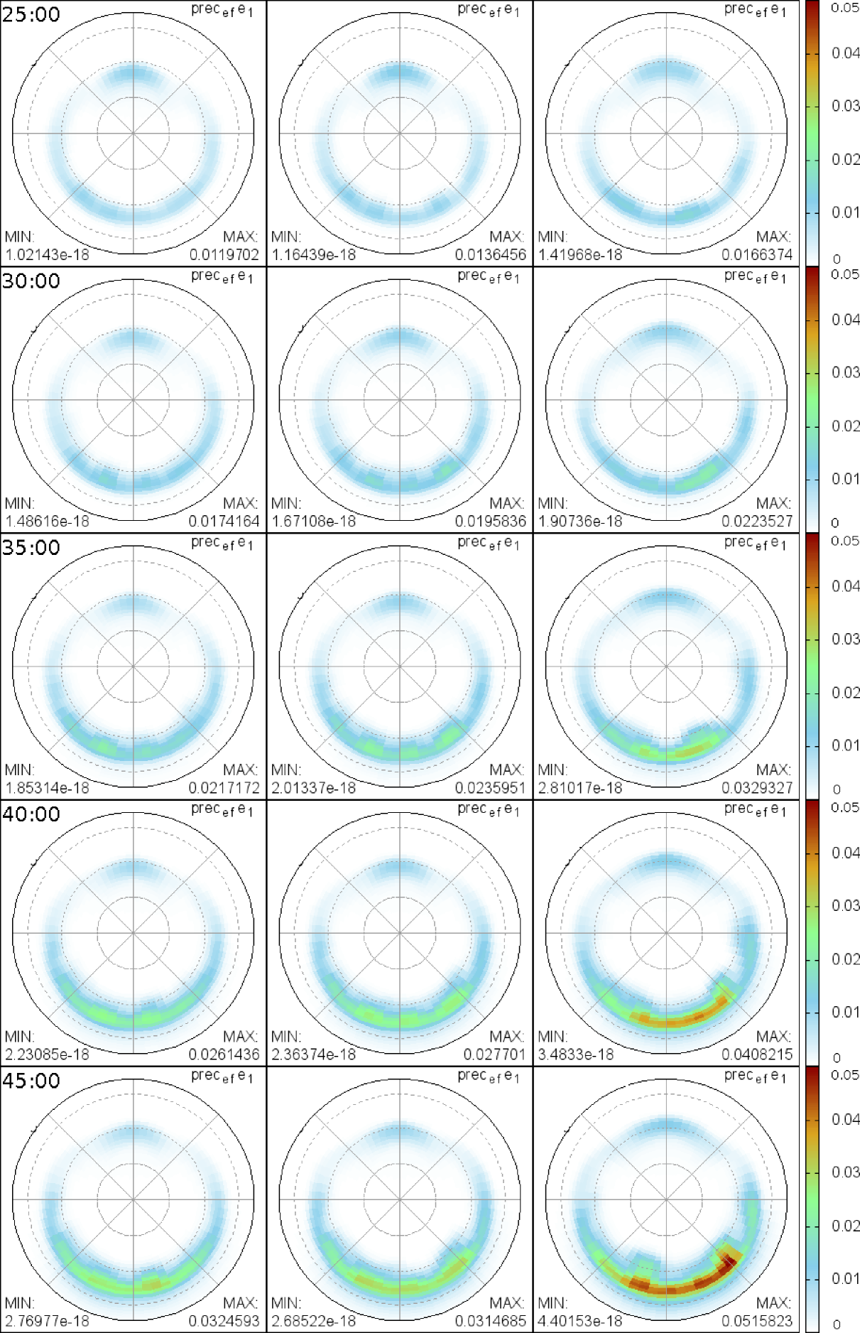
Figure 3 shows the diffusive auroral e- precipitation energy flux (DAPEF) in the time steps of 5 minutes from t = 25:00 minutes. In the IOS-1 and IOS-2 cases the DAPEF remained almost unaffected by the shock impact. In all cases, auroral precipitation is enhanced in the night side ionosphere approximately 12 minutes after shock impact. In the IOS cases, the shocks hit the magnetosphere behind the cusp, leading to a mild auroral precipitation at t = 35:00. However, at the same instant, the FPS enhances more auroral activity in the ionosphere nightside because the FPS impacts the magnetosphere behind the cusp, and thus the cusp is neither displaced nor compressed. In the FPS case, the shock hits the magnetosphere first at the nose, leading to a compression of the magnetosphere and the cusp, and to a pole-ward displacement of the cusp.
Later precipitation changes all occur in the nightside. As already shown by the FACs, these changes are mostly related to substorm activity. In the FPS case, auroral substorm onset is formed in the ionosphere nightside at 70 between 0300 MLT and 0600 MLT. Such auroral activity is not found in any IOS case.
In order to perform a quantitative comparison we integrate the ionosphere quantities over the northern hemisphere polar cap. To separate the directly driven response, which occurs mostly in the dayside, from the induced substorm response, which affects mostly the nightside, we integrate the FACs separately for the dayside and the nightside.
Figure 4 shows the time series of the integrated FACs, in MA, over the northern hemisphere ionosphere on both dayside (a) and nightside (b), for the three cases. In both panels, the blue lines indicate the IOS-1 case, the green lines indicate the IOS-2 case, and the red lines indicate the FPS case. The first vertical dashed line indicates the instance at which the IP shock hits the bow shock in the IOS-1 and IOS-2 cases, and the second vertical dashed line indicates that instance for the FPS case. The plotted quantity is the magnitude of the FAC, which is primarily the Region I current. As expected, the IP impact enhances the FACs on the dayside. Before the shock impact, the FACs on the dayside have nearly the same magnitude, 0.29 MA, and were in a quasi-steady state. In all cases, the dayside FAC magnitude begins to rise approximately 6 minutes after the shock impact. The FACs increase nearly linearly over a period of approximately 4 minutes, which corresponds roughly to the time it takes for the shock to pass over the dayside magnetosphere. This initial rise is nearly identical for all cases. Later, in the two IOS cases, the FAC remains by and large steady at around 0.5 MA for the IOS case, but continues to rise for another 20 minutes in the FPS case.
Figure 2 shows that the initial rise is in all cases due to enhanced FACs in the vicinity of the cusp. However, in the IOS-1 and IOS-2 cases the enhancement is mostly in the nightside of the cusp, whereas in the FPS case FACs both on the dayside and the nightside of the cusp are enhanced. It seems that the more thorough compression of the dayside magnetosphere leads to the stronger and more long lasting FAC enhancement in the FPS case, although that is not directly apparent in Figure 2.
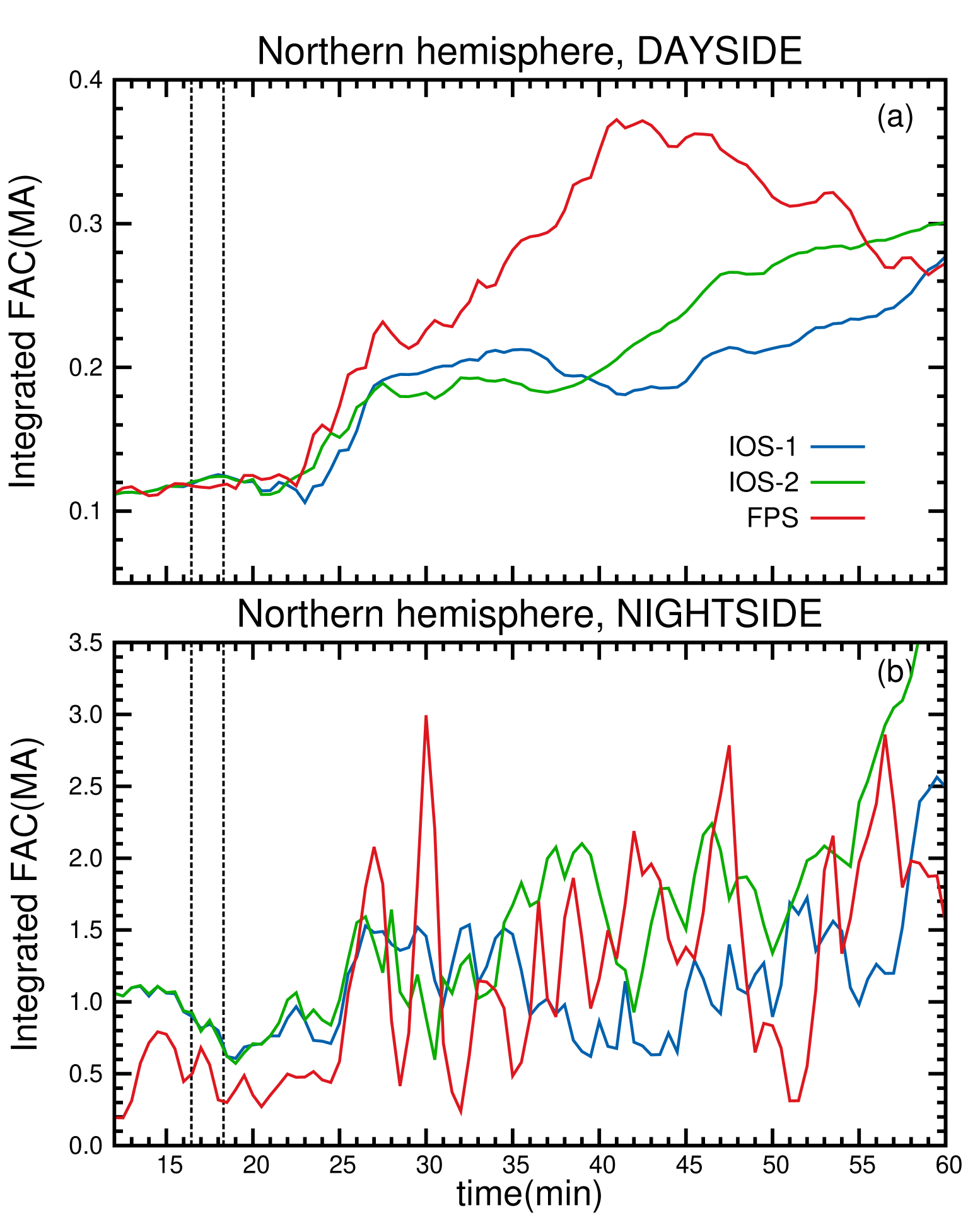
The nightside current enhancements (Figure 4 (b)) begin about 2 minutes after the dayside enhancements, in the three cases. For all shocks, the enhancements are qualitatively different from those on the dayside. In all cases, strong ULF waves are excited, with a period of 4-5 minutes. In the two IOS cases, the average FAC is enhanced from 2 MA to 3 MA due to the shock impact, with superimposed waves with an amplitude of the order of 0.2-0.3 MA. In the IOS-2 case, 17-18 minutes after the shock impact, the ULF wave amplitude rises to 0.75 MA. In the FPS case, the increase of the average FAC is similar, but the wave amplitude is much larger, i.e., of the order of 1-2 MA. These large oscillations persist for at least 60 minutes. While much of the response is similar to what Guo et al. (2005) found in their simulations, the oscillations are new. It is at present not clear what these oscillations correspond to in the magnetosphere, but they are likely cavity modes (Samson et al., 1992).
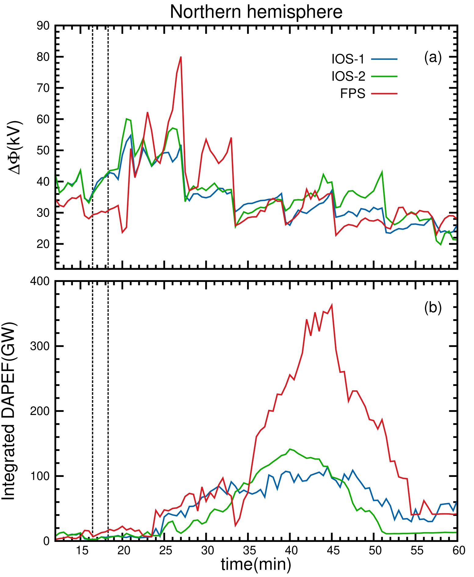
Figure 5 shows the cross polar cap potential (CPCP) and the integrated precipitation energy DAPEF in panels (a) and (b), respectively. DAPEF is calculated as the thermal energy flux of plasma sheet electrons assuming perfect pitch angle scattering, and a full loss cone (see Raeder et al., 1998; Raeder, 2003, for details).The blue line represents the IOS-1 case, the green line represents the IOS-2 case, and the red line represents the FPS case. Vertical, dashed lines, as described above, indicate the shock impact times for all cases. Before the shock impact, the system oscillated noticeably in an amplitude less than 5 kV in both cases. After the impact, the IOS-1 and IOS-2 induced a very similar potential jump from roughly 35 kV to a peak of approximately 55-60 kV. The CPCP oscillated with a period of nearly 5 minutes until it reached the near steady state value of 25 kV after 42 minutes.
The FPS case is more dynamic. The system oscillated around 30 kV before the shock impact. Right two minutes after the FPS hit the bow shock, the potential difference dropped to 23 kV. This effect was also seen by Guo et al. (2005) and interpreted as the redistribution of the FACs after the shock penetrates the magnetosphere. The potential drop then reached two smaller peaks, 50 kV at t=22:00 minutes, and 62 kV at t=24:00 minutes until it reached the maximum of 82 kV at t=27:00 minutes. The potential still reached two peaks of 53 kV at t=30:00 minutes and t=33:00 minutes. Then, the potential difference decreased in a period of nearly 7 minutes. After close to t=33:00 minutes, both systems evolved to nearly the same final quasi-steady state. This similarity has been shown by Guo et al. (2005) but not with this oscillatory behavior.
The bottom panel (b) of Figure 5 shows the time series for the integrated DAPEF, in units of GW. Again, the blue line represents the IOS-1 case, the green line represents the IOS-2 case, and the red line represents the FPS case. Before the shock impact the ionosphere is in a quiet state with low auroral activity. After the shock hit the bow shock, between t=24:00 minutes and t=33:00 minutes, the three systems evolved quite similarly, while the auroral energy flux suffered a small drop in the FPS case at t=34:00 minutes. In the IOS cases, the DAPEF attains a maximum value of barely 100-120 GW near t=44:00 minutes, and then evolves to a final state of 20-50 GW. On the other hand, the FPS enhanced the DAPEF much more, and briefly reaches a maximum of 350 GW at t=45:00 minutes.
By comparing the two shocks with the same Mach number, namely IOS-1 and FPS, we observe that both shocks lead to very different geomagnetic responses. Also, the IOS-2 geomagnetic response is smaller in comparison to the FPS geomagnetic response, even though the inclined shock was twice stronger than the head-on shock. We attribute these results to the different shock normal orientations. Comparison with Figure 3 shows that this enhanced precipitation flux must be from the nightside due to substorm activity. Such precipitation enhancements have been reported earlier by Zhou and Tsurutani (2001), Tsurutani and Zhou (2003), and Yue et al. (2010), who find that the auroral precipitation and field-aligned currents in the nightside can be intensified after a FFS impact, because it triggers the release of stored magnetospheric/magnetotail energy in the form of particularly large substorms, or even supersubstorms (See Tsurutani and Lakhina, 2014, for more references therein). Such substorm triggering might be a result of the decreasing in the nightside , as observed at geosynchronous orbit by Sun et al. (2011, 2012). In that case, the decrease in the nightside is suggested as a result of Earth-ward transportation of magnetic flux by temporarily enhanced plasma flows at the nightside geosynchronous orbit after the impingement of an IP shock. In our case, the symmetric plasma transport leads to a more intense geomagnetic activity. Although our simulations do not represent a storm and although the simulation results may be qualitatively in error, they match qualitatively the observed shock impact behavior.
4 Summary and Conclusions
It has been known for a long time that IP shocks can have a profound impact on the magnetosphere; however, it is much less known which factors determine the geoeffectiveness of IP shocks. There have been a few studies in the past addressing the effect of shock geometry (Takeuchi et al., 2002; Jurac et al., 2002; Guo et al., 2005; Wang et al., 2005, 2006; Grib and Pushkar, 2006; Samsonov, 2011), but none have considered the particular geometry that we investigated here. Specifically, here we use global simulations to contrast two different scenarios. In one scenario, the IP shock normal lies along the Sun-Earth line, such that there is a frontal impact on the magnetosphere. In the other scenario, the IP shock is inclined with respect to the Sun-Earth line. In either case, the shock normal lies in the GSE x-z plane, and the IMF is southward, such that there is no y-dependence of any solar wind parameter. The two scenarios lead to very different responses of the magnetosphere:
-
1.
In the frontal case, the shock launches waves symmetrically into the magnetosphere, which converge on the tail plasma sheet and compress it. By contrast, in the inclined cases, the waves reach the plasma sheet at different times, causing much less compression, but a north-south displacement of the plasma sheet. This result holds even for shocks with larger Mach numbers.
-
2.
In the frontal case, the compression triggers a substorm, whereas in the inclined cases there is no excess geomagnetic activity beyond what would be expected for southward IMF.
-
3.
In all cases the shock impact enhances FACs in the dayside with a similar quantitative response. However, in the inclined cases the FAC enhancement occurs mainly behind the cusp, whereas in the frontal case the cusp is displaced while the FACs increase over a wider MLT range. In the frontal case, the dayside FAC response also persists longer and is more intense, i.e., a 200% enhancement versus a 100% enhancement in the inclined case.
-
4.
The nightside FAC response is qualitatively similar in the three cases and shows the development of ULF waves. However, in the frontal case the ULF wave amplitude is much stronger. The detailed excitation mechanism remains to be investigated.
-
5.
The response of the cross polar cap potential is relatively benign and limited to the first 15 minutes after the impact, in all cases. The three cases relax to the pre-impact state in less than 20 minutes.
-
6.
In all cases diffuse auroral electron precipitation increases in similar fashion in direct response to the shock impact. In the frontal case, this is followed by a delayed response 10 minutes later, which peaks 20 minutes after the impact, and which comes from the nightside. The latter is interpreted as a consequence of the substorm triggered by the shock impact.
Our results show that the shock impact angle has a major effect on the geoeffectiveness of the shock, even more than the Mach number or some other measure of the shock strength. Although we only covered a relatively small parameter space in terms of impact angles, shock strength, and IMF orientation, the qualitative and quantitative differences we found are significant. With respect to substorm triggering (Kokubun et al., 1977; Lyons, 1995, 1996; Lui et al., 1990), the differences we found in the inclined and frontal cases are of particular importance. Apparently, the same type of IP shock can either trigger a substorm or not, depending on the shock normal direction, which has not been considered in previous studies. We also find large amplitude waves in the FACs that are apparently caused by the shock impacts. Given their period, these waves are likely cavity modes (Samson et al., 1992). We find that the modes have significantly larger amplitude for the frontal case. This is likely due to the fact that the waves that converge on the tail and compress the plasma sheet from there launch a wave back towards the nightside magnetosphere, which in turn excites the cavity mode. In the inclined cases, this earthward wave is likely much weaker, and thus excites a weaker cavity mode. We will study the wave excitation in more detail in a forthcoming paper. Other future work is also clearly laid out, namely finding the correlation between geomagnetic activity and IP shock normal orientation in data, and a better parameter space coverage with simulations.
Acknowledgements.
This work was supported by grant AGS-1143895 from the National Science Foundation and grant FA-9550-120264 from the Air Force Office of Sponsored Research. Computations were performed on Trillian, a Cray XE6m-200 supercomputer at UNH supported by the NSF MRI program under grant PHY-1229408. The artificial solar wind data input files from the simulations can be obtained from the corresponding author at dennymauricio@gmail.com.References
- Akasofu (1964) Akasofu, S.-I. (1964), The development of the auroral substorm, Planet. Space Sci., 12(4), 273–282, 10.1016/0032-0633(64)90151-5.
- Berdichevsky et al. (2000) Berdichevsky, D. B., A. Szabo, R. P. Lepping, A. F. Viñas, and F. Mariani (2000), Interplanetary fast shocks and associated drivers observed through the 23rd solar minimum by Wind over its first 2.5 years, J. Geophys. Res., 105(A12), 27,289– 27,314, 10.1029/1999JA000367.
- Bolduc (2002) Bolduc, L. (2002), GIC observations and studies in the Hydro-Québec power system, J. Atmos. Sol. Terr. Phys., 64(16), 1793–1802, 10.1016/S1364-6826(02)00128-1.
- Burlaga (1971) Burlaga, L. F. (1971), Hydromagnetic waves and discontinuities in the solar wind, Space Sci. Rev., 12(5), 600–657, 10.1007/BF00173345.
- Echer et al. (2003) Echer, E., W. D. Gonzalez, L. E. A. Vieira, A. D. L. F. L. Guarnieri, A. Prestes, A. L. C. Gonzalez, and N. J. Schuch (2003), Interplanetary shock parameters during solar activity maximum (2000) and minimum (1995-1996), Braz. Jour. Phys., 33(1), 2301, 10.1590/S0103-97332003000100010.
- Echer et al. (2004) Echer, E., M. V. Alves, and W. D. Gonzalez (2004), Geoefectiveness of interplanetary shocks during solar minimum (1995) and solar maximum (2000), Solar Phys., 221, 361–380, 10.1023/B:SOLA.0000035045.65224.f3.
- Fuller-Rowell et al. (1996) Fuller-Rowell, T. J., D. Rees, S. Quegan, R. J. Moffet, M. V. Codrescu, and G. H. Millward (1996), A coupled thermosphere-ionosphere model (CTIM), in STEP Report, edited by R. W. Schunk, p. 217, Scientific Commitee on Solar Terrestrial Physics (SCOSTEP), NOAA/NGDC, Boulder, Colorado.
- Ge et al. (2011) Ge, Y. S., J. Raeder, V. Angelopoulos, M. L. Gilson, and A. Runov (2011), Interaction of dipolarization fronts within multiple bursty bulk flows in global MHD simulations of a substorm on 27 February 2009, J. Geophys. Res., 116, A00I23, 10.1029/2010JA015758.
- Gilson et al. (2012) Gilson, M. L., J. Raeder, E. Donovan, Y. S. Ge, and L. Kepko (2012), Global simulation of proton precipitation due to field line curvature during substorms, J. Geophys. Res., 117(A5), 10.1029/2012JA017562.
- Grib and Pushkar (2006) Grib, S. A., and E. A. Pushkar (2006), Asymetry of nonlinear interactions of solar MHD discontinuities with the bow shock, Geomagnetism and Aeronomy, 46(4), 417–423, doi:10.1134/S0016793206040025.
- Guo and Hu (2007) Guo, X.-C., and Y.-Q. Hu (2007), Response of Earth’s ionosphere to interplanetary shocks, Chinese J. Geophys, 50(4), 817–823, 10.1002/cjg2.1099.
- Guo et al. (2005) Guo, X.-C., Y.-Q. Hu, and C. Wang (2005), Earth’s magnetosphere impinged by interplanetary shocks of different orientations, Chinese Phys. Lett., 22(12), 3221–3224, 10.1088/0256-307X/22/12/067.
- Hudson et al. (1997) Hudson, M. K., S. R. Elkington, J. G. Lyon, V. A. Marchenko, I. Roth, M. Temerin, J. B. Blake, M. S. Gussenhoven, and J. R. Wygant (1997), Simulations of radiation belt formation during storm sudden commencements, J. Geophys. Res., 102(A7), 14,087–14,102, 10.1029/97JA03995.
- Jeffrey and Taniuti (1964) Jeffrey, A., and T. Taniuti (1964), Nonlinear Wave Propagation, Academic Press, New York.
- Jurac et al. (2002) Jurac, S., J. C. Kasper, J. D. Richardson, and A. J. Lazarus (2002), Geomagnetic disturbances and their relationship to interplanetary shock parameters, Geophys. Res. Lett., 29(10), 10.1029/2001GL014034.
- Kappenman (2010) Kappenman, J. (2010), Geomagnetic storms and their impacts on the US power grid, Tech. rep., Metatech Corp., Goleta, California.
- Kokubun et al. (1977) Kokubun, S., R. L. McPherron, and C. T. Russell (1977), Triggering of substorms by solar wind discontinuities, J. Geophys. Res., 82(1), 74–86, 10.1029/JA082i001p00074.
- Koval et al. (2006) Koval, A., J. S̆afránková, Z. Nĕmec̆ek, A. A. Samsonov, L. Pr̆ech, and J. D. Richardson (2006), Interplanetary shock in the magnetosheath: Comparison of experimental data with MHD modeling, Geophys. Res. Lett., 33(L1102), 10.1029/2006GL025707.
- Lui et al. (1990) Lui, A. T. Y., A. Mankofsky, C.-L. Chang, K. Papadopoulos, and C. S. Wu (1990), A current disruption mechanism in the neutral sheet: A possible trigger for substorm expansions, J. Geophys. Res., 17(6), 745–748, 10.1029/GL017i006p00745.
- Lyons (1995) Lyons, L. R. (1995), A new theory for magnetospheric substorms, J. Geophys. Res., 100(A10), 19,069–19,081, 10.1029/95JA01344.
- Lyons (1996) Lyons, L. R. (1996), Substorms: Fundamental observational features, distinction from other disturbances, and external triggering, J. Geophys. Res., 101(A6), 13,011–13,025, 10.1029/95JA01987.
- Manchester et al. (2006) Manchester, W., A. Ridley, T. Gombosi, and D. DeZeeuw (2006), Modeling the Sun-to-Earth propagation of a very fast CME, Adv. Space Res., 38(2), 253–262, 10.1016/j.asr.2005.09.044.
- McPherron (1991) McPherron, M. L. (1991), Physical processes producing magnetospheric substorms and magnetic storms, in Geomagnetism, Volume 4, edited by J. Jacobs, Academic Press Ltd., Landing, Chapter 7.
- Oliveira (2014) Oliveira, D. (2014), Ionosphere-magnetosphere coupling and field-aligned currents, Revista Brasileira de Ensino de Física, 36(1), 1305, 10.1590/S1806-11172014000100005.
- Oliveira and Raeder (2013) Oliveira, D., and J. Raeder (2013), Role of symmetry in the geo–effectiveness of interplanetary shocks, in SM41B-2232, AGU Fall Meeting, San Francisco, CA.
- Parks (2004) Parks, G. K. (2004), Physics of Space Plasmas, Westview Press, Boulder, CO.
- Pizzo (1991) Pizzo, V. J. (1991), The evolution of corotating stream fronts near the ecliptic plane in the inner solar system: 2. Three-dimensional tilted-dipole fronts, J. Geophys. Res., 96(A4), 5405–5420, 10.1029/91JA00155.
- Priest (1981) Priest, E. F. (1981), Solar Magnetohydrodynamics, D. Reidel Publishing, Holland.
- Pulkkinen et al. (2011) Pulkkinen, A., K. Kuznetsova, A. Ridley, J. Raeder, A. Vapirev, D. Weimer, R. S. Weigel, M. Wiltberger, G. Millward, L. Rastätter, M. Hesse, H. J. Singer, and A. Chulaki (2011), Geospace environment modeling 2008-2009 challenge: Ground magnetic field perturbations, J. Geophys. Res., 9, 10.1029/2010SW000600.
- Pulkkinen et al. (2013) Pulkkinen, A., L. Rastatter, M. Kuznetsova, H. Singer, C. Balch, D. Weimer, G. Toth, A. Ridley, T. Gombosi, M. Wiltberger, J. Raeder, and R. Weigel (2013), Community-wide validation of geospace model ground magnetic field perturbation predictions to support model transition to operations, Space Weather, 11, 369, 10.1002/swe.20056.
- Raeder (2003) Raeder, J. (2003), Global Magnetohydrodynamics: A Tutorial Review, in Space Plasma Simulation, edited by J. Buchner, C. T. Dum, and M. Scholer, pp. 1–19, Springer Verlag, Berlin Heilderberg, New York, 10.1007/3-540-36530-311.
- Raeder and Lu (2005) Raeder, J., and G. Lu (2005), Polar cap potential saturation during large geomagnetic storms, Adv. Space Res., 36(1804), 10.1016/j.asr.2004.05.010.
- Raeder et al. (1998) Raeder, J., J. Berchem, and M. Ashour-Abdalla (1998), The Geospace Environment Modeling Grand Challenge: Results from a Global Geospace Circulation Model, J. Geophys. Res., 103(A7), 14,787–14,797, 10.1029/98JA00014.
- Raeder et al. (2001a) Raeder, J., Y. Wang, and T. J. Fuller-Rowell (2001a), Geomagnetic storm simulation with a Coupled Magnetosphere-Ionosphere-Thermosphere model, in Space Weather, Geophys. Monogr. Ser., vol. 125, edited by P. Song and H. J. Siscoe, pp. 377–384, American Geophysical Union, Washington, D.C., 10.1029/GM125p0377.
- Raeder et al. (2001b) Raeder, J., R. L. McPherron, L. A. Frank, S. Kokubun, G. Lu, T. Mukai, W. R. Paterson, J. B. Sigwarth, H. J. Singer, and J. A. Slavin (2001b), Global simulation of the Geospace Environment Modeling substorm challenge event, J. Geophys. Res., 106(A1), 381–395, 10.1029/2000JA000605.
- Raeder et al. (2008) Raeder, J., D. Larson, W. Li, E. L. Kepko, and T. Fuller-Rowell (2008), OpenGGCM simulations for the THEMIS mission, Space Sci. Rev., 141, 535–555, 10.1007/978-0-387-89820-9-22.
- Raeder et al. (2013) Raeder, J., P. Zhu, Y. Ge, and G. Siscoe (2013), Auroral signatures of ballooning mode near substorm onset: OpenGGCM simulations, in Auroral Phenomenology and Magnetospheric Processes: Earth And Other Planets, Geophys. Monogr. Ser., vol. 197, edited by A. Keiling, E. Donovan, and T. Karlson, pp. 389–396, American Geophysical Union, Washington, D.C., 10.1029/2011GM001200.
- Rastätter et al. (2013) Rastätter, L., M. M. Kuznetsova, A. Glocer, D. Welling, X. Meng, J. Raeder, M. Wiltberger, V. K. Jordanova, Y. Yu, S. Zaharia, R. S. Weigel, S. Sazykin, R. Boynton, H. Wei, V. Eccles, W. Horton, M. L. Mays, and J. Gannon (2013), Geospace Environment Modeling 2008-2009 challenge: Dst index, Space Weather, 11, 187, 10.1002/swe.20036.
- Richter et al. (1985) Richter, A. K., K. C. Hsieh, A. H. Luttrell, E. Marsch, and R. Schwenn (1985), Review of interplanetary shock phenomena near and within 1 AU, in Collisionless Shocks in the Heliosphere: Reviews of Current Research, Geophys. Monogr. Ser., vol. 35, edited by B. T. Tsurutani and R. G. Stone, pp. 33–50, American Geophysical Union, Washington, D.C., 10.1029/GM035p0033.
- Ridley et al. (2006) Ridley, A. J., D. L. De Zeeuw, W. B. Manchester, and K. C. Hansen (2006), The magnetospheric and ionospheric response to a very strong interplanetary shock and coronal mass ejection, Adv. Space Res., 38, 263–272, 10.1016/j.asr.2006.06.010.
- Russell et al. (1983) Russell, C. T., J. T. Gosling, R. D. Zwickl, and E. J. Smith (1983), Multiple spacecraft observations of interplanetary shocks: ISEE three-dimensional plasma measurements, J. Geophys. Res., 88(A12), 9941–9947, 10.1029/JA088iA12p09941.
- Russell et al. (2000) Russell, C. T., Y. L. Wang, J. Raeder, R. L. Tokar, C. W. Smith, K. W. Ogivie, A. J. Lazarus, R. P. Lepping, A. Szabo, H. Kawano, T. Mukai, S. Savin, Y. L. Yermolaev, X. Zhou, and B. T. Tsurutani (2000), The interplanetary shock of Septermber 24, 1998: Arrival at Earth, J. Geophys. Res., 105(A1), 25,143–25,154, 10.1029/2000JA900070.
- S̆afránková et al. (2007) S̆afránková, J., Z. Nĕmec̆ek, L. Pr̆ech, A. Samsonov, A. Koval, and K. Andréeovaá (2007), Interaction of interplanetary shocks with the bow shock, Planet. Space Sci., 55(15), 2324–2329, 10.1016/j.pss.2007.05.012.
- Samson et al. (1992) Samson, J. C., D. D. Wallis, T. J. Hughes, F. Creutzberg, J. M. Ruohoniemi, and R. A. Greenwald (1992), Substorm intensifications and field line resonances in the nightside magnetosphere, J. Geophys. Res., 97(A6), 8495–8518, 10.1029/91JA03156.
- Samsonov (2011) Samsonov, A. A. (2011), Propagation of inclined interplanetary shock through the magnetosheath, J. Atmos. Sol. Terr. Phys., 73, 10.1016/j.bbr.2011.03.031.
- Samsonov et al. (2006) Samsonov, A. A., Z. Nĕmec̆ek, and J. S̆afránková (2006), Numerical MHD modeling of propagation of interplanetary shock through the magnetosheath, J. Geophys. Res., 111(A082), 10.1029/2005JA011537.
- Samsonov et al. (2007) Samsonov, A. A., D. G. Sibeck, and J. Imber (2007), MHD simulation for the interaction of an interplanetary shock with the Earth’s magnetosphere, J. Geophys. Res., 112(A12220), 10.1029/2007JA012627.
- Samsonov et al. (2010) Samsonov, A. A., D. G. Sibeck, and Y. Yu (2010), Transient changes in magnetospheric-ionospheric current caused by the passage of an interplanetary shock: Northward interplanetary magnetic field case, J. Geophys. Res., 115(A05207), doi:10.1029/2009JA014751.
- Shi et al. (2013) Shi, Q. Q., M. Hartinger, V. Angelopoulos, Q.-G. Zong, X.-Z. Zhou, X.-Y. Zhou, A. Kellerman, A. M. Tian, J. Weygand, S. Y. Fu, Z. Y. Pu, J. Raeder, Y. S. Ge, Y. F. Wang, H. Zhang, and Z. H. Yao (2013), THEMIS observations of ULF wave excitation in the nightside plasma sheet during sudden impulse events, J. Geophys. Res., 118, 284–298, 10.1029/2012JA017984.
- Siscoe (1976) Siscoe, G. L. (1976), Three-dimensional aspects of interplanetary shock waves, J. Geophys. Res., 81(34), 6235–6241, 10.1029/JA081i034p06235.
- Sun et al. (2011) Sun, T. R., C. Wang, H. Li, and X. C. Guo (2011), Nightside geosynchronous magnetic field response to interplanetary shocks: Model results, J. Geophys. Res., 116(A4), 10.1029/2010JA016074.
- Sun et al. (2012) Sun, T. R., C. Wang, and Y. Wang (2012), Different Bz response regions in the nightside magnetosphere after the arrival of an interplanetary shock: Multipoint observations compared with MHD simulations, J. Geophys. Res., 117(A05227), 10.1029/2011JA017303.
- Takeuchi et al. (2002) Takeuchi, T., C. T. Russell, and T. Araki (2002), Effect of the orientation of interplanetary shock on the geomagnetic sudden commencement, J. Geophys. Res., 107(A12), 1423, 10.1029/2002JA009597.
- Tsurutani et al. (2011) Tsurutani, B., G. Lakhina, O. Verkhoglyadova, W. Gonzalez, E. Echer, and F. Guarnieri (2011), A review of interplanetary discontinuities and their geomagnetic effects, J. Atmos. Sol. Terr. Phys., 73(1), 5–19, 10.1016/j.jastp.2010.04.001.
- Tsurutani and Lakhina (2014) Tsurutani, B. T., and G. S. Lakhina (2014), An extreme coronal mass ejection and consequences for the magnetosphere and Earth, Geophys. Res. Lett., 41, 287–292, 10.1002/2013GL058825.
- Tsurutani and Zhou (2003) Tsurutani, B. T., and X. Y. Zhou (2003), Interplanetary shock triggering of substorms: Wind and Polar, Adv. Space Res., 31(4), 10.1016/S0273-1177(02)00796-2.
- Viñas and Scudder (1986) Viñas, A. F., and J. D. Scudder (1986), Fast and optimal solution to the “Rankine-Hugoniot” problem, J. Geophys. Res., 91(A1), 39–58, 10.1029/JA091iA01p00039.
- Wang et al. (2005) Wang, C., Z. H. Huang, Y. Q. Hu, and X. C. Guo (2005), 3D global simulation of the interaction of interplanetary shocks with the magnetosphere, in 4th Annual IGPP International Astrophysics Conference on the Physics of Collisionless Shocks, edited by G. Li, G. Zank, and C. T. Russell, pp. 320–324, AIP Conference Proceedings, Am. Inst. of Phys., Washington, D.C., 10.1063/1.2032716.
- Wang et al. (2006) Wang, C., C. X. Li, Z. H. Huang, and J. D. Richardson (2006), Effect of interplanetary shock strengths and orientations on storm sudden commencement rise times, Geophys. Res. Lett., 33(14), 10.1029/2006GL025966.
- Yue et al. (2010) Yue, C., Q. G. Zong, H. Zhang, Y. F. Wang, C. J. Yuan, Z. Y. Pu, S. Y. Fu, A. T. Y. Lui, B. Yang, and C. R. Wang (2010), Geomagnetic activity triggered by interplanetary shocks, J. Geophys. Res., 115(A5), 10.1029/2010JA015356.
- Zhou and Tsurutani (2001) Zhou, X., and B. T. Tsurutani (2001), Interplanetary shock triggering of nightside geomagnetic activity: Substorms, pseudobreakups, and quiescent events, J. Geophys. Res., 106(A9), 18,957–18,967, 10.1029/2000JA003028.
- Zong et al. (2009) Zong, Q.-G., X.-Z. Zhou, Y. F. Wang, X. Li, P. Song, D. N. Baker, T. A. Fritz, P. W. Daly, M. Dunlop, and A. Pedersen (2009), Energetic electron response to ULF waves induced by interplanetary shocks in the outer radiation belt, J. Geophys. Res., 114(A10), 10.1029/2009JA014393.