Impact of 16O(,)12C measurements on the 12C()16O astrophysical reaction rate
Abstract
The 12C()16O reaction, an important component of stellar helium burning, plays a key role in nuclear astrophysics. It has direct impact on the evolution and final state of massive stars, while also influencing the elemental abundances resulting from nucleosynthesis in such stars. Providing a reliable estimate for the energy dependence of this reaction at stellar helium burning temperatures has been a major goal for the field. In this work, we study the role of potential new measurements of the inverse reaction, 16O()12C, in reducing the overall uncertainty. A multilevel -matrix analysis is used to make extrapolations of the astrophysical factor for this reaction to the stellar energy of 300 keV. The statistical precision of the -factor extrapolation is determined by performing multiple fits to existing and ground state capture data, including the impact of possible future measurements of the 16O()12C reaction. In particular, we consider a proposed Jefferson Laboratory (JLab) experiment that will make use of a high-intensity low-energy bremsstrahlung beam that impinges on an oxygen-rich single-fluid bubble chamber in order to measure the total cross section for the inverse reaction. The importance of low energy data as well as high precision data is investigated.
I Introduction
The 12C()16O reaction is believed to be one of the most important reactions in nuclear astrophysicsFowler (1984); Woosley et al. (2003). A recent reviewdeBoer et al. (2017) highlights the key role played by this reaction in both the evolution of and nucleo-synthetic yields from massive stars. The purpose of this study is to explore the role that forthcoming measurements of the inverse reaction - 16O()12C (OSGA) - could have on reducing the overall uncertainty in the cross section for the 12C()16O reaction at helium burning temperatures. To do this we perform fits to the existing data using the -matrix approachLane and Thomas (1958) and study the impact of including new data on the inverse reaction. This is achieved by starting with a reasonable -matrix fit that can be used as a basis for comparison to fits with and without projected 16O()12C data. For the inverse capture data we start with a proposed JLab experimentSuleiman et al. (2013) in order to assess the possible role of new measurements in reducing the overall uncertainty in the cross sectionHolt et al. (2018). A detailed -matrix analysis of this reaction and and excellent review of the subject is given in Ref.deBoer et al. (2017).
In the present work, we employed the -matrix approach to calculate the total cross section, , for alpha-capture to the ground state. Considering only ground state capture is sufficient for this study since the capture to excited states is believeddeBoer et al. (2017) to contribute only about 5 to the total capture rate at 300 keV. The cross section is then used to calculate the astrophysical factor given by
| (1) |
where is the energy in the center of mass, is the Sommerfeld parameter, , and is the reduced mass of the carbon ion and alpha particle. Measurements of the factor as a function of energy are often reported in the literature. For the 12C()16O reaction, the value of at is typically quoted as the most probable energy for stellar helium burning. Of course, the cross section is so small at 300 keV that it cannot be directly measured. Thus, extrapolations to 300 keV must be performed to study the impact of data on the extrapolation. Of course, efforts aimed at improving the data and extrapolation are underwaySuleiman et al. (2013); Gai (2018); Balabanski et al. (2017); Costantini et al. (2009); Robertson et al. (2016); Liu (2017); Bemmerer et al. (2018); Xu et al. (2007); Friščić et al. (2019) at a number of laboratories worldwide. The new inverse reaction (OSGA) experimentsSuleiman et al. (2013); Xu et al. (2007); Gai (2018); Balabanski et al. (2017); Friščić et al. (2019) bring a different set of systematic errors than previous experiments and thus provide an additional check on systematics.
II -matrix approach
The collision matrix for the OSGA reaction will be given in terms of the Hamiltonian which electromagnetically couples the photon of multipolarity to the nucleus. We introduce the wave function that describes the alpha-12C system in total spin state and an initial state wave function which describes the nucleus (16O) in its ground state. Then the collision matrix is given by
| (2) |
where is the photon wave number and the subscript c refers to the final C channel with quantum numbers . Here is the channel spin (zero in this case), is the orbital angular momentum, and is the total angular momentum. In principle, we would perform the radial integration in Eq. 2 from the origin to the channel radius (internal piece) and from the channel radius to infinity (external piece). According to the R-matrix theoryLane and Thomas (1958) inside the channel radius , the final state wave function, , can be expanded in terms of a complete set of states,
| (3) |
where is a Coulomb phase shift, is the width of level in channel , and is the matrix that relates the internal wave function and the observed resonances. Here
| (4) |
where is a level energy, is the Kronecker and is given in terms of the Coulomb shift factor, , the boundary condition constant, , and the Coulomb penetration factor,
| (5) |
where here c refers to essentially the channel in this case and the are the reduced width amplitudes. The channel is the only open channel and closed channels are neglected.
The internal part of the collision matrix for radiative capture to the ground state is given by
| (6) |
where is the Coulomb phase shift for orbital angular momentum , and are the formal ground state and radiative widths, respectively. For a given level, the observed width can be relatedLane and Thomas (1958) to the reduced width by
| (7) |
while the reduced widths for the bound states are given by
| (8) |
where is the bound state shift factor for orbital angular momentum . For the photon radiative width, we have
| (9) |
where is the observed radiative width and
| (10) |
where is the -value for the reaction and are the physical resonance energies as given in the equation .
We then calculated the ground state radiative cross sectionCarr and Baglin (1971) for the 12C(,)16O reaction from the collision matrix for spin-zero nuclei:
| (11) |
We only considered ground state transitions and statistical errors in this study. We initially chose a channel radius of 5.43 fm to be consistent with a previous analysisdeBoer et al. (2017), but later consider a larger channel radius to be consistent with other analysesKirsebom et al. (2018); Shen et al. (2019). We employed five resonance levels and four resonance levels in the internal part of the the R-matrix analysis as shown in Table 1. This analysis is similar to that of refs.Azuma et al. (2010) and Holt et al. (1978), and the details comport with the results of Lane and ThomasLane and Thomas (1958). In order to speed up computations, we turned off the external part for this study. This external contribution is most sensitive to the part of the cross section since the external part is greatly reduced by isospin symmetry. In fact, the external E1 part would vanish under perfect isospin conservation. We performed the fit for data less than 3 MeV, where the external part is small. As a check, we turned on the external piece for several fits, but it did not significantly change the results.
| Eλ | Eλ | |||||
|---|---|---|---|---|---|---|
| (MeV) | (keV) | (eV) | (MeV) | (keV) | (eV) | |
| 1 | -0.297 | 114.6∗ | 0.055 | -0.482 | 105.0∗ | 0.097 |
| 2 | 2.416 | 414.7∗ | -0.0152∗ | 2.683 | 0.62 | -0.0057 |
| 3 | 5.298 | 99.2 | 5.6 | 4.407 | 83.0 | -0.65 |
| 4 | 5.835 | -29.9 | 42.0 | 6.092 | -349 | -1.21∗ |
| 5 | 10.07 | 500 | 0.604∗ | - | - | - |
III Simultaneous fits and projections for , and total
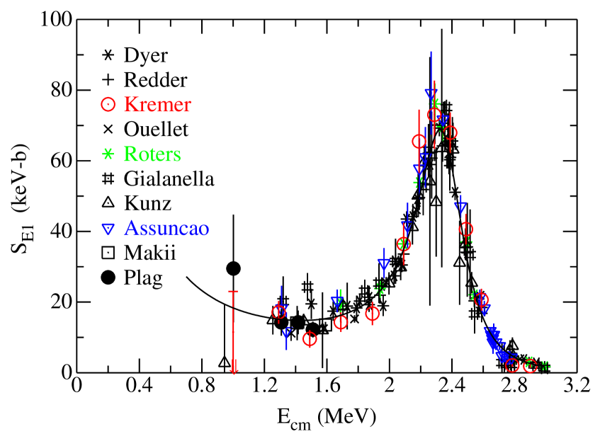
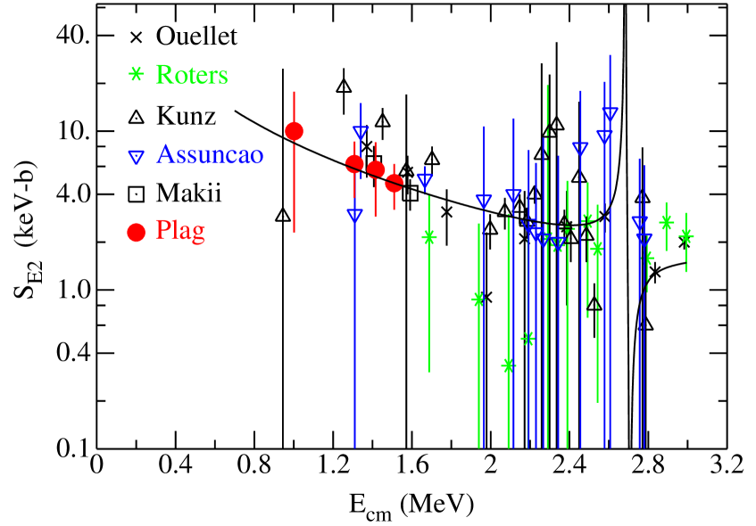
We used a SIMPLEX fitterNelder and Mead (1965) for the present work. Our best -matrix fit of the existing and -factor data, shown in Fig. 1, was taken as the most probable description of the -factor data. In order to explore the statistical variation in the S-factor extrapolations, we created -factor pseudo-data by random variation according to a Gaussian probability distribution about the best fit -factor values at the measured energies. In the randomizations, we multiplied the individual pseudo-data uncertainties by the square root of the ratio of the original best fit values to the original measured uncertainties. We further multiplied these uncertainties by the square root of the and reduced chi squares, the Birge factorBirge (1932), for the and fits, respectively. This procedure should give a conservative estimate for statistical uncertainties. For the subtheshold states, we fixed the radiative widths of the subthreshold states at the measured values and varied the reduced alpha widths. We allowed the reduced alpha and radiative width of the first state above threshold to vary in the fit, while we allowed the radiative width of the fifth state to vary. We also allowed the radiative width of the fourth R-matrix level to vary. The first state above threshold is very narrow and we fixed the parameters of this level at those of ref.deBoer et al. (2017). The radiative width of the third resonance was treated separately. We observed that using the value in ref.deBoer et al. (2017) resulted in a cross section that was significantly smaller than the data of ref.Schurmann et al. (2011). Rather, we made a fit to data that included the data of ref.Schurmann et al. (2011). We then fixed the third radiative width at -0.65 eV found from the fit and used it in subsequent fits to the data below 3 MeV. Indeed, we fixed all other parameters except the third radiative width and those marked with an asterisk in Table 1 at the values of ref.deBoer et al. (2017). The parameters allowed to vary are denoted by an asterisk in table 1.
Also, following ref. deBoer et al. (2017), we performed the fits by maximizing L rather than minimizing , where L is givenSivia and Skilling (2006) by
| (12) |
and is the usual quantity used in minimizations. Here is the function to be fitted to data, , with statistical error . The L maximization has the feature that it reduces the impact of large error bar data on the fit and generally gives larger S-factor uncertainties in projected values of than that of a minimization. In this work is maximized and defined by
| (13) |
where is for data and represents for the inverse reaction data or JLab data in this case.
The parameters of the bound levels are very important for the projection to 300 keV. The resonance energies were fixed, but the parameters, , depend on the reduced width of the levels. We allowed the reduced widths of the bound states to vary, so the varies. We chose the -matrix boundary condition constants to cancel out this effect for the second levels so that for these levels. For the third and higher levels, the reduced widths were not varied because alpha elastic scattering determined these widths and allowing them to vary did not make a significant difference. We used the -factor data sets given in refs. Dyer and Barnes (1974); Kremer et al. (1988); Redder et al. (1987); Ouellet et al. (1992); Roters et al. (1999); Gialanella et al. (2001); Kunz et al. (2001); Assuncao et al. (2006); Makii et al. (2009); Plag et al. (2012) and show the E1 and E2 ground state S factors in Fig.1.
III.1 Fits with a channel radius of 5.43 fm
Proposed OSGA experimentsSuleiman et al. (2013); Ugalde et al. (2013); DiGiovine et al. (2015); Gai (2018); Balabanski et al. (2017) are expected to have several orders of magnitude improvement in luminosity over previous experiments and should provide data at the lowest practical values of energy. We take our best -matrix fit of the and -factor data as the most probable description of the projected JLab data. We then randomly varied these OSGA -factor pseudo data based on their projected uncertainties according to a Gaussian probability distribution about the best fit -factor values. The parameters that were used to provide the matrix curves shown in Fig. 1 are given for reference in Table 1. In order to study the impact of proposed OSGA data and low energy data in particular, we performed five fits: a fit to existing and data (denoted by “all” in Table 2); a fit to data published after the year 2000 (denoted by “2000”), both with (denoted by “J” in table 2) and without projected JLab data; and a fit to all data in Fig. 1 above 1.6 MeV (denoted by “1.6” in table 2). Although it has been customaryPérez et al. (2017) to eliminate data sets that deviate by more than three standard deviations from the fitted results, we chose to select data sets after the year 2000 as a test of systematic deviations and as suggested by StriederStrieder (2018). This approach assumes that experimental equipment and methods have improved over the decades. Another reason for this approach is that not all authors of the data sets disclose their systematic errors. The factors projected to 300 keV along with standard deviations, , which represent the statistical fit uncertainty are given in Table 2 for the five cases. The reduced for the fit to the original data is also shown. As a test of the method, we arbitrarily reduced the error bars for the projected JLab data by an order of magnitude and present the results as “all J/10” in the table.
Several observations can be made from Table 2. The standard deviations for the total projected -factors with proposed JLab data are generally smaller than those without JLab data. The total and projections appear to be significantly larger for 1.6 MeV data than the fits to “all” data, indicating the importance of low-energy data. As expected the standard deviations for the “all J/10” case are significantly smaller than that for the other cases. For the fits to the data after 2000, the reduced is significantly smaller than that for fits to “all” data. This indicates that the data sets after 2000 are more consistent with one another than with all data sets. Finally, the -factor projections for appear to be about a third of those for E1.
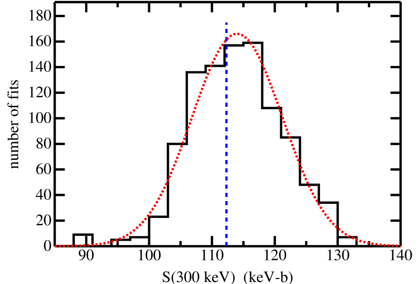
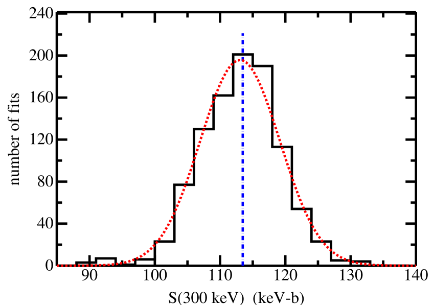
As an example, the projections from the simultaneous fit to all and data, the case represented by the first line in Table 2, are shown in Fig. 2. The dashed vertical line indicates the projection for the fit to the original data, while the histogram represents the results of fits to 1000 sets of randomized pseudo-data. The dotted curve is a Gaussian based on the mean and standard deviation found from the fits. The (300 keV) from the fit to original data is 112.3 keV-b while the mean for the fits to pseudo-data is 114.0 keV-b. The standard error for the fits to pseudo-data is about 0.2 keV-b. Thus, the statistical error in the fits to 1000 sets of pseudo-data cannot alone explain the discrepancy. If one speculates that the systematics in the original data are driving the discrepancy, then we could compare the “2000” data. The (300 keV) for the fit to the “2000” data is 123.5 keV-b, while the mean of the pseudo-data fits is 123.2 keV-b, in better agreement with one another.
| data | orig | ||||||
|---|---|---|---|---|---|---|---|
| (keV-b) | |||||||
| all | 2.3 | 112.3 | 7.2 | 77.6 | 6.4 | 34.7 | 2.8 |
| all J | 2.2 | 113.5 | 6.1 | 81.8 | 5.8 | 31.7 | 3.0 |
| 2000 | 1.7 | 123.5 | 6.9 | 89.6 | 6.4 | 33.9 | 3.3 |
| 2000 J | 1.7 | 125.0 | 6.7 | 89.7 | 6.3 | 35.2 | 3.4 |
| 1.6 | 2.6 | 119.6 | 5.8 | 87.1 | 5.4 | 32.5 | 2.6 |
| all J/10 | 2.4 | 116.4 | 2.4 | 81.1 | 3.5 | 35.3 | 1.9 |
| all J/2 | 2.2 | 118.8 | 4.2 | 81.8 | 3.9 | 37.2 | 2.8 |
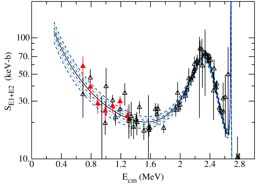
Fig. 3 shows the curves that represent 1,2 and 3 standard deviation simultaneous fits to existing and data. We generated the curves by performing 500 fits to the data, generating 500 sets of parameters similar to those in Table 1, and then using the parameter sets to determine the standard deviation at each value of energy. The representative capture data, shown as open triangles, were taken as the sum of and results governed by where both and data exist. The projected JLab data are represented by red triangles in the figure. Given the statistical errors for the projected JLab data and the small number of values, one might not expect the projected JLab data to have a large impact on the statistical error. Although the impact of new JLab data cannot easily be seen from this figure, reducing the expected JLab errors by only a factor of two could make a significant impact as illustrated by the last line in Table 2.

In order to more quantitatively explore the efficacy of the proposed JLab data, we made 1000 fits to a varying number of projected JLab data points from one to seven points beginning with the highest energy point 1190 keV and ending with the lowest energy point 590 keV. These results are shown in Fig. 4. Note that we generated the JLab data as before by the fit values with a channel radius of 5.43 fm to “all” data, then randomizing, according to the projected statistical errors. We repeated this procedure with the JLab projected statistical errors divided by two as well as by ten. These results are also shown in Fig. 4. The higher precision data indicate a clear pattern of diminishing returns in terms of the standard deviations as a function of the cumulative number of projected JLab data points. This pattern is not so clear for the actual proposed JLab statistical errors.
III.2 Fits with a channel radius of 6.5 fm
As mentioned before some previous -matrix analyses have used a channel radius of 6.5 fm. In order to be consistent with these previous analyses, we set the channel radius at 6.5 fm, and as before, we performed five fits: a fit to existing and data (denoted by “all” in table 3); a fit to data published after the year 2000 (denoted by “2000”), both with (denoted by “J” in Table 3) and without projected JLab data; and a fit to all data in Fig. 1 above 1.6 MeV (denoted by “1.6” in Table 3). The factors projected to 300 keV along with standard deviations, , are given in Table 3 for the five cases. The reduced for the fit to the original data is also shown. As with the 5.43 fm case, the standard deviations for the total projected -factors with proposed JLab data are generally smaller than those without JLab data. Again, the total and projections appear to be significantly larger for 1.6 MeV data than the fits to “all” data, and the size of the difference substantially exceeds the statistical errors. As can be seen from comparing Tables 2 and 3, the -factor projections to 300 keV are generally larger for a channel radius of 6.5 fm than those for 5.43 fm. This finding is consistent with that of ref deBoer et al. (2017). Again, the fit to data sets after 2000 also exhibit a smaller reduced than that for “all” data. It is interesting to note that if the errors on the expected 7 JLab data points are reduced by a factor of two, the case presented in the last line of Table 3, then the result is in agreement with the 5.43 fm case, the first line in Table 2. This indicates that high quality data at low energy could even bring fits with different channel radii into agreement at least with regard to the extrapolation to 300 keV.
| data | orig | ||||||
|---|---|---|---|---|---|---|---|
| (keV-b) | |||||||
| all | 2.3 | 124.9 | 8.3 | 80.6 | 7.1 | 44.3 | 5.0 |
| all J | 2.2 | 121.7 | 6.3 | 84.3 | 5.9 | 37.4 | 2.8 |
| 2000 | 1.6 | 131.3 | 8.3 | 90.5 | 7.7 | 40.7 | 3.8 |
| 2000 J | 1.6 | 131.3 | 7.2 | 90.5 | 6.9 | 40.7 | 3.8 |
| 1.6 | 2.4 | 136.9 | 8.6 | 102.5 | 8.1 | 34.3 | 3.1 |
| all J/2 | 2.3 | 116.0 | 5.7 | 76.5 | 6.2 | 39.5 | 3.2 |
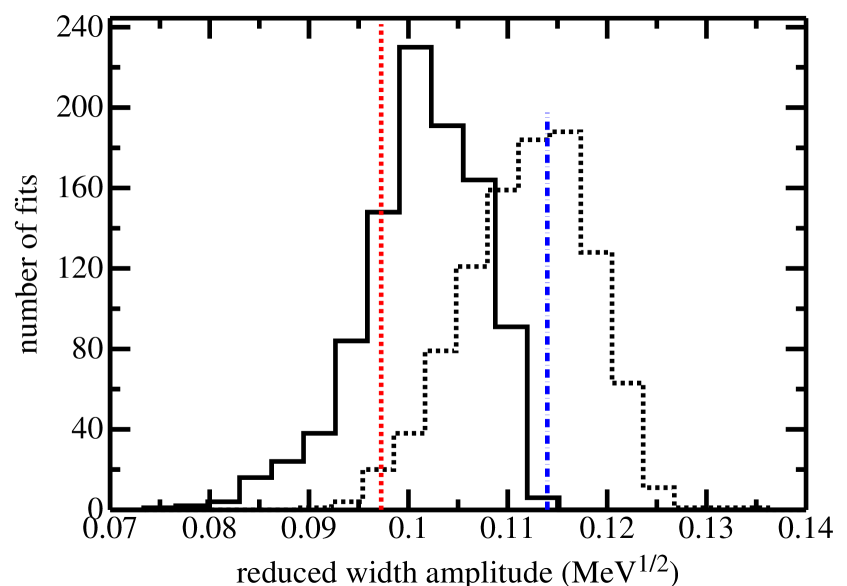
The bound p-wave reduced width amplitudes found from the fits to “all” and “1.6” MeV data for a channel radius of 6.5 fm are given in Fig. 5. The histograms from the fits shown in the figure are asymmetric indicating that the error is not a Gaussian distribution. The reduced width amplitudes of the bound - and -wave states, and the quantity found from the fits are given in Table 4 along with a recent value found from the 16N() processKirsebom et al. (2018) for the bound -wave state and for a transfer reactionShen et al. (2019) for the bound -wave state. Here, the quantity , where is the p-wave penetration factor evaluated at 300 keV, was included in table 4 in order to better compare with that of ref Kirsebom et al. (2018). As pointed out in ref. Kirsebom et al. (2018) the quantity is the dominant term in the capture cross section. The present fits give values of that are consistent with the experiment and analysis of ref. Kirsebom et al. (2018) although the channel radius of ref. Kirsebom et al. (2018) is 6.35 fm. The fits to data above 1.6 MeV (“1.6”) give results that are larger for the -wave state and smaller for the -wave state than that for the other results. Again, this indicates the importance of low energy data. The fit for the after 2000 data that includes projected JLab data “2000 J” reduces the statistical error somewhat for the bound -wave state. It is noted that while the (300) of 46.2 7.7 keV-b found from a recent transfer reactionShen et al. (2019) is in excellent agreement with the (300) from the present analysis with a 6.5 fm channel radius for “all” data as indicated in Table 3, the reduced width for the bound state for the “all” case differs by about two-sigma between these two approaches.
| Fit or data | |||
|---|---|---|---|
| (MeV1/2) | (eV) | (MeV1/2) | |
| all | 0.097() | 4.68() | 0.150(9) |
| 2000 | 0.104(() | 5.38() | 0.142(8) |
| 1.6 | 0.114(() | 6.46() | 0.130(6) |
| 16N() | - | 5.17(75)(54) | - |
| 12C(11B,7Li)16O | - | - | 0.134(18) |
IV Summary
From this study it appears that inverse reaction data can have a significant impact on the projection of (300 keV) based on the projected OSGA data. We took the projected JLab data to represent + data since only total cross sections to the ground state will be measured. The projected standard deviation for the 1000 fits to the and data with the proposed JLab data is generally smaller than that without JLab data. The JLab data constrain the total + cross section in the fit. This leads to smaller standard deviations than fitting and separately. Fitting only data above 1.6 MeV leads to a significant shift upward in the projected -factors at 300 keV. This illustrates the importance of lower energy data in the extrapolation to 300 keV. Since the expected OSGA data will be less than 1.6 MeV and even lower than existing data, we can infer that the proposed OSGA data will have a significant impact on the value of the low energy extrapolation. The significant difference between (300 keV) for the fits with channel radii of 5.43 and 6.5 fm indicates model uncertainty. The lower energy OSGA data may help resolve this ambiguity. For example, if the uncertainties on the projected 7 JLab data points are reduced by a factor of two, the (300 keV) from a fit with a 5.43 fm channel radius is brought into agreement with that from a 6.5 fm fit. This level of accuracy at low energies would represent an interesting goal not only for the upcoming JLab experiment, but also for the other future experiments.
Acknowledgements.
We thank O. Kirsebom and F. Strieder for useful discussions. This work is supported by the U.S. National Science Foundation under grant 1812340 and by the U.S. Department of Energy (DOE), Office of Science, Office of Nuclear Physics, under contract No. DE-AC02-06CH11357References
- Fowler (1984) W. A. Fowler, Rev. Mod. Phys. 56, 149 (1984).
- Woosley et al. (2003) S. E. Woosley, A. Heger, T. Rauscher, and R. D. Hoffman, Nucl. Phys. A718, 3 (2003).
- deBoer et al. (2017) R. deBoer et al., Rev. Mod. Phys. 89, 035007 (2017), arXiv:1709.03144 [nucl-ex] .
- Lane and Thomas (1958) A. M. Lane and R. G. Thomas, Rev. Mod. Phys. 30, 257 (1958).
- Suleiman et al. (2013) R. Suleiman et al., (2013), Jefferson Lab Proposal PR12-13-005.
- Holt et al. (2018) R. J. Holt, B. W. Filippone, and S. C. Pieper (2018) arXiv:1809.10176 [nucl-ex] .
- Gai (2018) M. Gai, 41th Symposium on Nuclear Physics (Cocoyoc2018) Cocoyoc, Mexico, January 8-11, 2018, J. Phys. Conf. Ser. 1078, 012011 (2018).
- Balabanski et al. (2017) D. L. Balabanski, R. Popescu, D. Stutman, K. A. Tanaka, O. Tesileanu, C. A. Ur, D. Ursescu, and N. V. Zamfir, EPL 117, 28001 (2017).
- Costantini et al. (2009) H. Costantini, A. Formicola, G. Imbriani, M. Junker, C. Rolfs, and F. Strieder, Rept. Prog. Phys. 72, 086301 (2009), arXiv:0906.1097 [nucl-ex] .
- Robertson et al. (2016) D. Robertson, M. Couder, U. Greife, F. Strieder, and M. Wiescher, Proceedings, 13th International Symposium on Origin of Matter and Evolution of the Galaxies (OMEG2015): Beijing, China, June 24-27, 2015, EPJ Web Conf. 109, 09002 (2016).
- Liu (2017) W. P. Liu, Proceedings, 14th International Symposium on Nuclei in the Cosmos (NIC-XIV): Niigata, Japan, June 19-24, 2016, JPS Conf. Proc. 14, 011101 (2017).
- Bemmerer et al. (2018) D. Bemmerer et al., in 5th International Solar Neutrino Conference Dresden, Germany, June 11-14, 2018 (2018) arXiv:1810.08201 [physics.acc-ph] .
- Xu et al. (2007) Y. Xu, W. Xu, Y. G. Ma, W. Guo, Y. G. Chen, X. Z. Cai, H. W. Wang, C. B. Wang, G. C. Lu, and W. Q. Shen, Nucl. Instrum. Meth. A581, 866 (2007).
- Friščić et al. (2019) I. Friščić, T. W. Donnelly, and R. G. Milner, (2019), arXiv:1904.05819 [nucl-ex] .
- Carr and Baglin (1971) R. W. Carr and J. E. E. Baglin, Atom. Data Nucl. Data Tabl. 10, 143 (1971).
- Kirsebom et al. (2018) O. S. Kirsebom et al., Phys. Rev. Lett. 121, 142701 (2018), arXiv:1804.02040 [nucl-ex] .
- Shen et al. (2019) Y. P. Shen et al., Phys. Rev. C99, 025805 (2019), arXiv:1811.06220 [nucl-ex] .
- Azuma et al. (2010) R. E. Azuma et al., Phys. Rev. C81, 045805 (2010).
- Holt et al. (1978) R. J. Holt, H. E. Jackson, Jr, R. M. Laszewski, J. E. Monahan, and J. R. Specht, Phys. Rev. C18, 1962 (1978).
- Nelder and Mead (1965) J. A. Nelder and R. Mead, Comput. J. 7, 308 (1965).
- Birge (1932) R. T. Birge, Phys. Rev. 40, 207 (1932).
- Schurmann et al. (2011) D. Schurmann et al., Phys. Lett. B703, 557 (2011).
- Sivia and Skilling (2006) D. Sivia and J. Skilling, Data Analysis: A Baysian Tutorial, 2nd ed. (Oxford University Press, Oxford, 2006).
- Dyer and Barnes (1974) P. Dyer and C. A. Barnes, Nucl. Phys. A233, 495 (1974).
- Kremer et al. (1988) R. M. Kremer, C. A. Barnes, K. H. Chang, H. C. Evans, B. W. Filippone, K. H. Hahn, and L. W. Mitchell, Phys. Rev. Lett. 60, 1475 (1988).
- Redder et al. (1987) A. Redder, H. W. Becker, C. Rolfs, H. P. Trautvetter, T. R. Donoghue, T. C. Rinckel, J. W. Hammer, and K. Langanke, Nucl. Phys. A462, 385 (1987).
- Ouellet et al. (1992) J. M. L. Ouellet et al., Phys. Rev. Lett. 69, 1896 (1992).
- Roters et al. (1999) G. Roters, C. Rolfs, F. Strieder, and H. Trautvetter, Eur. Phys. J. A 6, 451 (1999).
- Gialanella et al. (2001) L. Gialanella et al., Nucl. Phys. A688, 254 (2001).
- Kunz et al. (2001) R. Kunz, M. Jaeger, A. Mayer, J. W. Hammer, G. Staudt, S. Harissopulos, and T. Paradellis, Phys. Rev. Lett. 86, 3244 (2001).
- Assuncao et al. (2006) M. Assuncao et al., Phys. Rev. C73, 055801 (2006).
- Makii et al. (2009) H. Makii, Y. Nagai, T. Shima, M. Segawa, K. Mishima, H. Ueda, M. Igashira, and T. Ohsaki, Phys. Rev. C80, 065802 (2009).
- Plag et al. (2012) R. Plag, R. Reifarth, M. Heil, F. Kappeler, G. Rupp, F. Voss, and K. Wisshak, Phys. Rev. C86, 015805 (2012).
- Ugalde et al. (2013) C. Ugalde, B. DiGiovine, D. Henderson, R. J. Holt, K. E. Rehm, A. Sonnenschein, A. Robinson, R. Raut, G. Rusev, and A. P. Tonchev, Phys. Lett. B719, 74 (2013), arXiv:1212.6819 [astro-ph.IM] .
- DiGiovine et al. (2015) B. DiGiovine, D. Henderson, R. J. Holt, R. Raut, K. E. Rehm, A. Robinson, A. Sonnenschein, G. Rusev, A. P. Tonchev, and C. Ugalde, Nucl. Instrum. Meth. A781, 96 (2015), arXiv:1501.06883 [nucl-ex] .
- Pérez et al. (2017) R. N. Pérez, J. E. Amaro, and E. Ruiz Arriola, Phys. Rev. C95, 064001 (2017), arXiv:1606.00592 [nucl-th] .
- Strieder (2018) F. Strieder, private communication (30 May 2018).