Impact of Spectral Resolution on -index and Its Application to Spectroscopic Surveys
Abstract
Utilizing the PHOENIX synthetic spectra, we investigated the impact of spectral resolution on the calculation of -indices. We found that for spectra with a resolution lower than 30,000, it is crucial to calibrate -indices for accurate estimations. This is especially essential for low-resolution spectral observations. We provided calibrations for several ongoing or upcoming spectroscopic surveys such as the LAMOST low-resolution survey, the SEGUE survey, the SDSS-V/BOSS survey, the DESI survey, the MSE survey, and the MUST survey. Using common targets between the HARPS and MWO observations, we established conversions from spectral -indices to the well-known values, applicable to stars with [Fe/H] values greater than 1. These calibrations offer a reliable approach to convert -indices obtained from various spectroscopic surveys into values and can be widely applied in studies on chromospheric activity.
1 Introduction
The Ca II H and K lines are two strong resonance lines in stellar optical spectra. The line wings could be modeled using local thermodynamic equilibrium (LTE), thereby unveiling the temperature structure of the photosphere. (Rutten et al., 2004; Sheminova, 2012; Rouppe van der Voort, 2002). Meanwhile, the reversed structure and central absorption profile at the line center, caused by rising temperature and source function’s decoupling from the Planck function, respectively, can serve as diagnosis of temperature structures of both lower and upper chromosphere (Vernazza et al., 1981; Leenaarts et al., 2013; Bjørgen et al., 2018).
Detailed modeling of the emission cores of Ca II H and K lines suggests that they are sensitive to magnetic fields, which is also confirmed by solar observations (Babcock & Babcock, 1955; de la Cruz Rodríguez et al., 2013; Cretignier et al., 2024). Naturally they are excellent tracers of solar active regions (Sowmya et al., 2023; Cretignier et al., 2024), solar or stellar flares (Reiners, 2009; Pietrow et al., 2024) and the 11-year solar cycle (Sheeley, 1967; Dineva et al., 2022).
Acting as pioneer, Wilson (1968) carried out a campaign to monitor the flux of the stellar Ca II H and K lines using the 100-inch telescope at the Mount Wilson Observatory (MWO), which was equipped with a two-channel photometer, named as HKP-1. Later on Vaughan et al. (1978) designed a four channel spectrometer named as HKP-2 and put it on the 60-inch telescope at MWO to avoid the instrumental effects of HKP-1.
Initially, slits with full width at half maximum (FWHM) of 1.09 Å were applied for observing dwarfs. Later on, the slits were replaced by new devices to allow the choice between 1 Å and 2 Å window (Duncan et al., 1991), with the later is more suitable for observing giants considering the Wilson-Bappu effect, which leads to wider emission cores of Ca II H and K lines compared to dwarfs (Wilson & Vainu Bappu, 1957). These observations provided an elite sample with long-term monitoring of stellar Ca II H and K activity levels, confirming that the stellar Ca II H and K lines could also vary quasi-periodically (Wilson, 1978).
The chromospheric contribution to the Ca II H and K lines was first defined as the observed flux of Ca II H and K line cores with a basal flux to be subtracted, which was derived from a sample of inactive stars (Wilson, 1968). Later on, Vaughan et al. (1978) proposed the well-known Mount Wilson -index () to quantify the chromospheric activity, defined as . and are the background-corrected counts in the H band centered at 3968.47 Å and K band centered at 3933.664 Å, respectively. and denote the background-corrected counts within the 20 Å ranges of [3991.067 Å, 4011.067 Å] and [3891.067 Å, 3911.069 Å], respectively. is the normalizing factor used to correct instrumental effects between HKP-1 and HKP-2 so that the -indices are equal to the mean flux of the Ca II H and K lines (Vaughan et al., 1978). The index has been widely used as an indicator of stellar chromospheric activity.
Subsequent spectral observations calculated the spectra-based -indices following a similar equation: . H and K represent integrated flux corresponding to the H and K lines. The integration window was a triangle bandpass with a FWHM of 1.09 Å. R and V are the integrated flux in the two 20 Å rectangle reference bands at red and violet sides of H and K lines. The 8 is a correction factor for the longer exposure times of the V and R bandpass of the HKP-2 instrument.
However, the value reported in the literature for different instruments vary significantly (e.g., Gray et al., 2006; Hall et al., 2007; Boro Saikia et al., 2018). Generally, the value can be obtained by comparing the -indices of the same stars observed by the MWO and other spectral surveys, allowing spectra-based -indices to be converted to the Mount Wilson scale (i.e., ) for consistent comparison. Unfortunately, the stars observed by the MWO are typically bright, whereas current spectroscopic surveys increasingly target fainter stars. As a result, there are often few stars in common between the MWO observations and a given spectroscopic survey. Therefore, it would be highly worthwhile to establish a straightforward and promising method to determine the conversion relations for different spectroscopic surveys.
Some instrumental effects including the spectral resolution, CCD response, ghosts and filter throughput could potentially influence the line profiles (e.g. Suzuki et al., 2003; Adibekyan et al., 2020; Dumusque et al., 2021; Cretignier et al., 2021; Pietrow et al., 2024), among which the spectral resolution plays an important role. In this paper, we aim to use the PHOENIX synthetic spectra (Husser et al., 2013) to investigate the impact of spectral resolution on the calculation of -index. Furthermore, we will present the conversion relations between spectra-based -indices and across different spectral resolutions, especially for some wide-field spectroscopic surveys, including the LAMOST (Cui et al., 2012; Luo et al., 2015), the SEGUE (Yanny et al., 2009), the SDSS-V (Kollmeier et al., 2017), the DESI (DESI Collaboration et al., 2016), and some upcoming surveys like the Maunakea Spectroscopic Explorer sky survey (MSE; Hill et al., 2018) and the MUltiplexed Survey Telescope sky survey (MUST; Zhao et al., 2024). The paper is organized as follows. In section 2 we introduce the data and method. Results and discussions are presented in Section 3.
2 Data and Method
2.1 PHOENIX synthetic spectra
PHOENIX high-resolution synthetic spectra have a resolution of 500,000. They are modeled under the local thermodynamic equilibrium (LTE), with non-LTE corrections applied for some specific lines including the Ca II H and K lines (Husser et al., 2013). The library covers a range of effective temperatures () from 2300 K to 12,000 K, surface gravities (log) from 0 to 6, and metallicities ([Fe/H]) from 4 to 1. In this work, we mainly focused on late-type dwarf and giant stars so that we only used the synthetic spectra with between 2500 K and 6500 K and log between 2 and 6. Meanwhile, all [Fe/H] grids have been included. No -enhancement was considered. We treated targets with log larger than 3.5 as dwarfs and those with log smaller than 3.5 as giants. Meanwhile, we marked targets with K as F-type stars, K as G-type stars, K as K-type stars, and K as M-type stars.
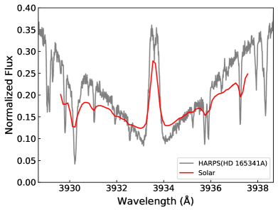
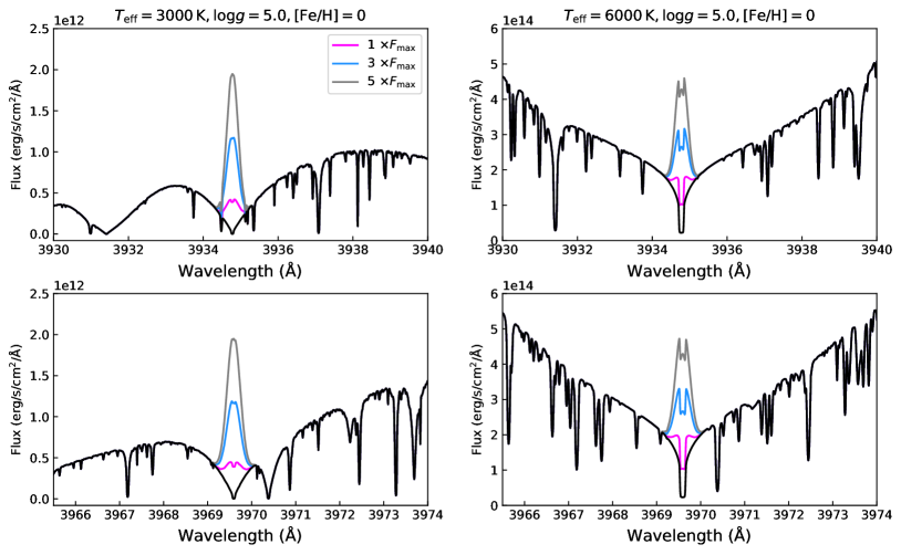
To simulate spectra with chromospheric activity, we first constructed two normalized Gaussian profiles centered at 3934.78 Å and 3969.59 Å. In order to derive the full width at half maximum (FWHM) corresponding to stellar activity, we first conducted an estimation of the FWHM for the emission cores of the Ca II H and K lines using HARPS spectra111http://archive.eso.org/wdb/wdb/adp/phase3_main/form for several active stars and the spectrum of solar spot region (Cretignier et al., 2024). In Figure 1 we plot two examples. The gray spectrum corresponds to HD 165341A (K0V), observed with HARPS while the red spectrum is the solar spectrum at the spot region (Cretignier et al., 2024). The results suggest that an FWHM of 0.35 Å matches well with the observed spectra. As a result, in this work the FWHM of each Gaussian profile was set to be 0.35 Å. These Gaussian profiles were then scaled by a group of factors, ranging from 1 to 10 with steps of 1, multiplying the maximum flux within the wavelength range between 3800 Å and 4100 Å, respectively, to represent different levels of chromospheric activity. Finally, these Gaussian profiles were added to the PHOENIX spectra. Figure 2 provides some examples.
2.2 Calculation of -index
We calculated the -index following
| (1) |
excluding the factors of 8 and . H and K represent the integrated fluxes corresponding to the H and K bands, centered at 3969.59 Å and 3934.78 Å, respectively. Note that these wavelengths mark the vacuum cores of the Ca II H and K lines. The integration window for these bands was a triangle bandpass with a FWHM of 1.09 Å. R and V refer to the integrated fluxes within two 20 Å rectangle reference bands on the red and violet sides of H and K lines, centered at 4001 Å and 3901 Å, respectively. In addition, considering the Wilson-Bappu effect, which indicates that the widths of the emission line cores of the Ca II H and K lines are broader in giants compared to dwarfs (Wilson & Vainu Bappu, 1957), we also used a 2.18 Å integration range for the and bands to calculate the -indices for giants. It is worth noticing that a wider bandpass would wash out the weaker activity signal since more photospheric contribution from the wings would be brought in (Gomes da Silva et al., 2022; Pietrow et al., 2024).
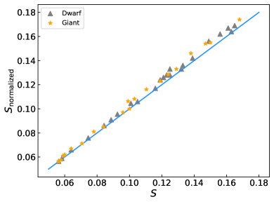
It should be noted that we used the original PHOENIX spectra (with flux units of erg/s/Å/cm2) for the calculations, while in many observations, normalized spectra were used (e.g. Wright et al., 2004; Schröder et al., 2009; Han et al., 2024). Therefore, we first conducted a check to see whether the -indices calculated from normalized and unnormalized spectra are the consistent. We randomly selected a group of templates with various and log values and fixed [Fe/H] values of 0.0. The comparison of the -indices shows only a minor deviation, suggesting that both methods yield consistent results (Figure 3).
We first calculated the -indices for the original PHOENIX spectra with a resolution of and labeled them as . Then, the spectra were convolved to various resolutions of , 2000, 3000, 4000, 5000, 6000, 7000, 7500, 8000, 9000, 10,000, 15,000, 20,000, 30,000, 50,000, and 100,000 using a Gaussian window, and the corresponding -indices were calculated, labeled as . For giants, the -indices calculated using 2.18 Å window were denoted as . There are a total of 22,140 dwarf templates and 11,070 giant templates at each resolution. These calculations will be used to investigate the influence of spectral resolution on the values of -indices.
3 Results and Discussions
3.1 The effects of spectral resolution
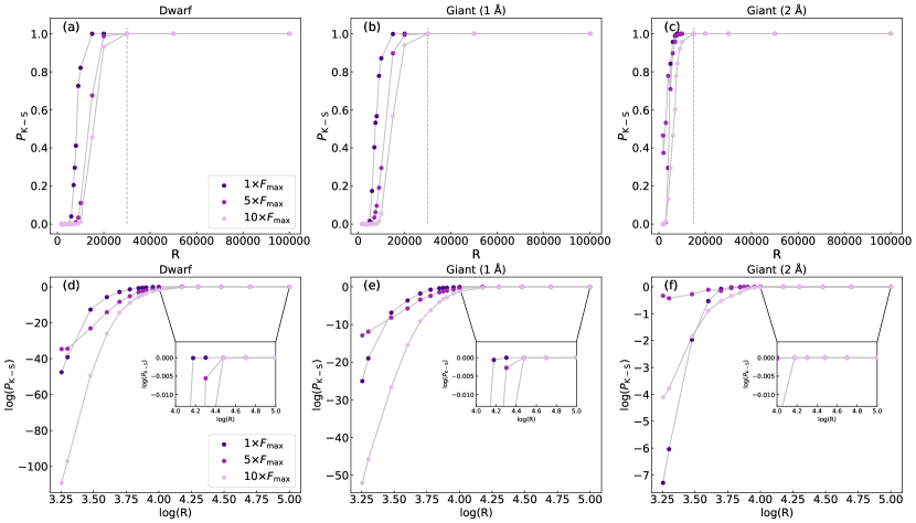
We used the standard nonparametric Kolmogorov-Smirnov (K-S) test to quantitatively assess at which resolution the and samples can be treated as the same. Generally, the two samples can be regarded as different if the null hypothesis probability is much smaller than one. To be conservative, here we treat they as the same if 0.99.
It is obvious that at low resolutions, the and samples are significantly different (Figure 4). Moreover, at the same resolution, the difference become more notable as the Ca II H and K emission levels increase, indicating that stronger emission lines could amplify the impact of resolution. Conversely, at high resolution, the two samples are quite consistent.
For both dwarfs and giants with -indices calculated using a 1.09 Å window, the knee point, where the and samples can be considered consistent, is around . For giants with -indices calculated with a 2.18 Å window, the knee point is about . We proposed that for spectra with , the effects of resolution on -index estimation can be ignored (i.e., ). Our results are roughly consistent with Bouchy et al. (2001) who proposed a 50,000 resolution threshold. The difference in threshold may be due to the different wavelength ranges. Bouchy et al. (2001) used a wider wavelength range to investigate the influence of spectral resolution on line profile while we only focused on the narrow emission cores of Ca II H and K lines.
3.2 Conversion from to
Considering the impact of spectral resolution on the calculation of -indices, especially for low-resolution cases, one should convert the values to values to mimic the resolution effects. Here we provide the calibrations for some large spectroscopic sky surveys, including the LAMOST low-resolution survey with (Cui et al., 2012), the SEGUE survey with (Yanny et al., 2009), the SDSS-V/BOSS survey with (Kollmeier et al., 2017), the DESI survey with (DESI Collaboration et al., 2016), and some upcoming sky surveys like the MSE survey with (Hill et al., 2018) and the MUST survey with (Zhao et al., 2024).
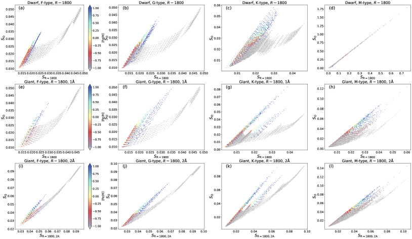
Figure 5 shows the comparison of and for different types of stars. For stellar templates with [Fe/H] , the and exhibit a linear relationship, whereas for templates with [Fe/H] , the relationship becomes non-linear. Since the integration window includes the line wings, the slope of the wings will affect the flux within the integrated region. For metal-rich stars, their broad wings have shallower slopes, making the integration less sensitive to slope variations. As a result, changes in metallicity, which affect the slopes, only have a minor impact on the integrated flux and thus lead to tight relations between and . In contrast, metal-poor stars exhibit narrower line wings with steeper slopes. Consequently, the integrated flux becomes more sensitive to the wings, and changes in slopes caused by variations in [Fe/H] significantly influence the integrated flux. This results in large dispersions in the - relations.
After excluding metal-poor stars, the relations are similar across different types of stars and the correlation is tighter for late-type stars. Therefore, we will focus our analysis on the relations for stellar templates with [Fe/H] . In addition, our analysis reveals that excluding A- to M-type stars with [Fe/H] from the LAMOST DR10 catalog reduces the target sample by merely 4, suggesting that the excluding of these stars will not significantly influence the statistical analysis. For templates with [Fe/H] , although there are small differences in the - relations, we treat them as a single group.
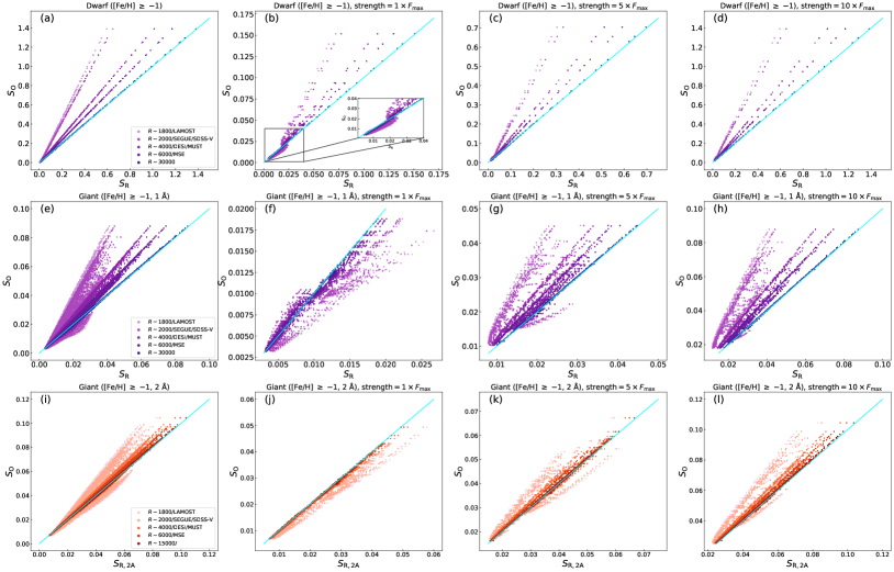
Figure 6 compares and for dwarfs with a 1.09 Å widow, giants with a 1.09 Å window and giants with a 2.18 Å window, respectively. Obviously, the deviation between and gradually increases as the spectral resolution decreases. Additionally, for both dwarfs and giants, when the emission levels of Ca II H and K lines are high, the relationships are very tight. However, when the emission levels are low, the relations would split into several branches in low-resolution cases (e.g., ).
For each resolution, a linear regression was applied to fit the relationship between and using templates with [Fe/H] with all the emission strengths:
| (2) |
Furthermore, for low-resolution spectra, we divided the sample into two groups based on activity levels: a low-activity group ( 0.02 for dwarfs and 0.01 for giants) and a high-activity group ( 0.02 for dwarfs and 0.05 for giants). Individual linear regression was applied to each group. The fitting results are listed in table 1. These individual fittings are recommended for -index calibrations. Additionally, for the low-activity group, we performed linear fittings for different types of stars, and the fitting results were found to be very similar. Finally, since the linear relations are tighter when calculating the -indices using a 2.18 Å compared to those that correspond to 1.09 Å window (Figure 6), as reported by Duncan et al. (1991); Schröder et al. (2018), we suggested to use a 2.18 Å window to calculate the -indices for giants.
3.3 Conversion from to
The -indices represent the total emission of the Ca II H and K lines, which includes the photospheric contribution unrelated to magnetic activity. To address this, the , which represents the “flux excess” in the Ca II H and K lines, was introduced as the standard chromospheric activity indicator. It can be derived from the through a series of complex steps (Noyes et al., 1984; Mittag et al., 2013). In the following analysis we will provide conversions from to .
In Section 3.2, we presented the conversions from to . Establishing the relationship between and would become straightforward only if we can determine the relationship between and . Since is consistent with (Section 3.1) we can use stars common to high-resolution spectroscopic surveys and the MWO observations to derive these relationship.
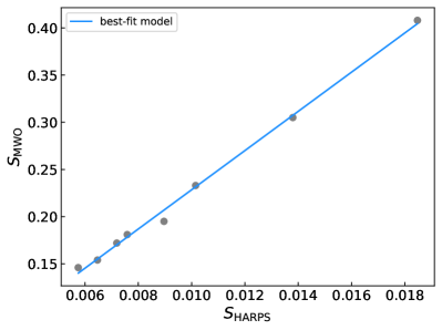
Fortunately, there are some common sources between the HARPS spectral observations and the MWO observations (Boro Saikia et al., 2018). The HARPS spectra, with a very high resolution of 120,000, allow the to be treated as without requiring further calibration for resolution effects. All these spectra were corrected for radial velocities using the values provided by the HARPS data-reduction software (Pepe et al., 2002). For each target, we normalized all the spectra and calculated the -indices of HARPS spectra with . The median value of these measurements for each source was adopted as the final result (i.e., ). We then applied a linear regression to values and values from Boro Saikia et al. (2018) following
| (3) |
The fitting coefficients are and . Since were not multiplied by a factor of 8, the fitting results are differ from those reported by Boro Saikia et al. (2018). Figure 7 shows the fitting results.
Finally, we provided the general relations between and as follows,
| (4) |
The results of and for each resolution are summarized in table 1.
| Type | Resolution | Activity level | Stellar Type | ||||
|---|---|---|---|---|---|---|---|
| Dwarf (1 Å) | 1800 | All | All | 2.37 | 0.021 | 49.2181.221 | 0.4150.012 |
| All | 2.413 | 0.026 | 50.1111.243 | 0.5190.014 | |||
| All | 1.461 | 0.005 | 30.3410.753 | 0.0830.006 | |||
| F | 1.81 | 0.014 | 37.5880.932 | 0.270.009 | |||
| G | 1.973 | 0.015 | 40.9731.016 | 0.2910.009 | |||
| K | 1.695 | 0.007 | 35.20.873 | 0.1250.006 | |||
| M | 1.524 | 0.006 | 31.6490.785 | 0.1040.006 | |||
| 2000 | All | All | 2.166 | 0.018 | 44.9811.116 | 0.3530.01 | |
| All | 2.196 | 0.021 | 45.6041.131 | 0.4150.012 | |||
| All | 1.435 | 0.005 | 29.8010.739 | 0.0830.006 | |||
| F | 1.758 | 0.013 | 36.5080.905 | 0.2490.008 | |||
| G | 1.861 | 0.013 | 38.6470.958 | 0.2490.008 | |||
| K | 1.634 | 0.006 | 33.9330.841 | 0.1040.006 | |||
| M | 1.477 | 0.005 | 30.6730.761 | 0.0830.006 | |||
| 4000 | All | All | 1.381 | 0.005 | 28.6790.711 | 0.0830.006 | |
| 6000 | All | All | 1.192 | 0.002 | 24.7540.614 | 0.0210.005 | |
| Giant (1 Å) | 1800 | All | All | 1.641 | 0.004 | 34.0790.845 | 0.0620.005 |
| All | 1.734 | 0.006 | 36.010.893 | 0.1040.006 | |||
| All | 1.909 | 0.005 | 39.6440.983 | 0.0830.006 | |||
| F | - | - | - | - | |||
| G | - | - | - | - | |||
| K | 2.071 | 0.006 | 43.0081.067 | 0.1040.006 | |||
| M | 1.694 | 0.004 | 35.1790.872 | 0.0620.005 | |||
| 2000 | All | All | 1.646 | 0.005 | 34.1820.848 | 0.0830.006 | |
| All | 1.755 | 0.007 | 36.4460.904 | 0.1250.006 | |||
| All | 1.789 | 0.004 | 37.1520.921 | 0.0620.005 | |||
| F | - | - | - | - | |||
| G | - | - | - | - | |||
| K | 1.93 | 0.005 | 40.080.994 | 0.0830.006 | |||
| M | 1.601 | 0.003 | 33.2480.825 | 0.0420.005 | |||
| 4000 | All | All | 1.34 | 0.003 | 27.8280.69 | 0.0420.005 | |
| 6000 | All | All | 1.184 | 0.002 | 24.5880.61 | 0.0210.005 | |
| Giant (2 Å) | 1800 | All | All | 1.134 | 0.002 | 23.550.584 | 0.0210.005 |
| All | 1.123 | 0.002 | 23.3210.579 | 0.0210.005 | |||
| All | 1.154 | 0.003 | 23.9650.594 | 0.0420.005 | |||
| F | - | - | - | - | |||
| G | - | - | - | - | |||
| K | 1.264 | 0.004 | 26.2490.651 | 0.0620.005 | |||
| M | 1.02 | 0.001 | 21.1820.525 | 0.00.005 | |||
| 2000 | All | All | 1.137 | 0.002 | 23.6120.586 | 0.0210.005 | |
| All | 1.137 | 0.002 | 23.6120.585 | 0.0210.005 | |||
| All | 1.12 | 0.002 | 23.2590.577 | 0.0210.005 | |||
| F | - | - | - | - | |||
| G | - | - | - | - | |||
| K | 1.226 | 0.003 | 25.460.631 | 0.0420.005 | |||
| M | 0.996 | 0.0 | 20.6840.513 | 0.0210.005 | |||
| 4000 | All | All | 1.084 | 0.001 | 22.5110.558 | 0.00.005 | |
| 6000 | All | All | 1.05 | 0.001 | 21.8050.541 | 0.00.005 |
3.4 Application to LAMOST
The LAMOST low-resolution spectra have been widely used in the studies of stellar magnetic activity (e.g. Zhang et al., 2020a, b; Li et al., 2024; Ye et al., 2024; Zhang et al., 2021). Some studies (e.g., Karoff et al., 2016) calculated the -indices as and simply treated it as to derive following the method of Mittag et al. (2013). Although the authors adopted as the calibration factor, their approach may introduce inaccuracies in the results. Furthermore, Karoff et al. (2016) used the air wavelength to define the line centers of the Ca II H and K lines, whereas the LAMOST spectra are provided in vacuum wavelengths. Given the low resolution of LAMOST spectra, this 1 Å difference could strongly affect the calculation of .
The most appropriate approach is to first convert to and then calculate . However, there are no common targets between the LAMOST and MWO observations. Consequently, Li et al. (2024) and Han et al. (2024) used common targets between the LAMOST and HARPS observations to do the calibration using the HARPS -indices (Boro Saikia et al., 2018), subsequently converting them into . Similarly, Zhang et al. (2022) used common stars between the LAMOST observations and the catalog given by Duncan et al. (1991), while Zhang et al. (2024) utilized common targets between the LAMOST observations and several catalogs with -indices calibrated to the MWO measurement.
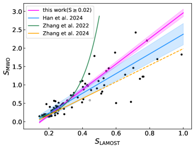
To compare our results with the conversion relations derived observationally, we plotted the relations from Zhang et al. (2022), Zhang et al. (2024), and Han et al. (2024) in Figure 8. The coefficients (i.e., slopes and intercepts) of the linear relations are 2.68 and in Han et al. (2024) or 2.26 and 0.27 for solar-like stars (5400 K 6500 K) in Zhang et al. (2024). Note that the LAMOST -indices calculated in these studies were multiplied by a factor of , which explains why their coefficients differ from our results in table 1. Additionally, Zhang et al. (2022) used an exponential function to fit the relationship between and for solar-like stars. Since both the relations from Zhang et al. (2022) and Zhang et al. (2024) only include solar-like stars with , their relations differ from our results. The magenta line in Figure 8 corresponds to the model with and for dwarfs with and . The fitting result is different from those from previous literature, especially at large region.
The differences of the relations may be caused by the biased sample, since there are only a few targets with large -indices. In previous studies, which provided calibrations from observations, they may be suffered from sample selection bias, low signal-to-noise ratio, and low resolution that could lead to the inaccuracy in the measurement of radial velocities and thus influence the determining of line centers. These effects would lead to large uncertainties while converting to observationally (For example the blue shaded area in Figure 8).
3.5 Other Effects
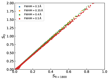
First, in this work we used a 0.35 Å Gaussian profile to simulate stellar activity. However, different structures and physical processes in the chromosphere, including the velocity gradients of the fluid, the intensity of shock wave and the non-LTE radiative transfer, would influence the widths of line cores (e.g. Carlsson & Stein, 1997). To test the potential influence, in Figure 9 we plot the relations of and corresponding to various FWHM of emission cores, i.e., 0.3 Å, 0.35 Å, 0.4 Å, and 0.5 Å. Obviously, the relations are similar. We conclude that when the simulated emission cores are within the integrated windows, the fitting result will not change significantly.
Second, the rotational broadening may also have notable impact on the line profile. We further tested the effect using a representative stellar model with K, log 4.5 and [Fe/H] 0.0, corresponding to a K-type dwarfs. Assuming a typical radius of 0.7 and a very short rotation period of 1 day, we derived a FWHM of 0.5 Å of the simulated emission core, which is still smaller than the typical width of integrated window. Thus the rotational broadening will not affect our results significantly.
4 Summary
In this study, we examined the influence of spectral resolution on the calculation of -indices using PHOENIX synthetic spectra. We calculated values at the original resolution of PHOENIX spectra and values after convolving the spectra to a resolution of 1800, 2000, 3000, 4000, 5000, 6000, 7000, 7500, 8000, 9000, 10,000, 15,000, 20,000, 30,000, 50,000, and 100,000. For dwarf stars, the -indices were calculated with a 1.09 Å bandpass, while for giant stars, the -indices were calculated in both 1.09 Å bandpass and 2.18 Å bandpass. Our analysis revealed that lower resolutions led to larger discrepancies between the and values. Below a spectral resolution of 30,000, it is necessary to calibrate -indices for accurate estimations. For giant stars analyzed within a 2.18 Å window, this threshold shifts to a resolution of 15,000.
We also provided calibrations from to values for several current or upcoming spectroscopic surveys, including the LAMOST low-resolution survey with , the SEGUE survey with , the SDSS-V/BOSS survey with , the MUST survey with , the DESI survey with , and the MSE survey with . These calibrations were conducted specifically for templates with [Fe/H] values higher than 1, since templates with lower metallicity do not exhibit a linear relationship between and . Additionally, we categorized the templates into high-activity and low-activity groups based on their -indices and developed the scaling relations for each group separately. For low-activity groups, although we divided them into several subgroups, the activity region as well as the differences of their scaling relations are small. Therefore for relations in table 1, we recommend to use those with stellar type = “All”. More importantly, using common targets between the HARPS and MWO observations, we established conversions from to , which can be widely applied in studies focusing on chromospheric activity.
References
- Adibekyan et al. (2020) Adibekyan, V., Sousa, S. G., Santos, N. C., et al. 2020, A&A, 642, A182
- Babcock & Babcock (1955) Babcock, H. W., & Babcock, H. D. 1955, ApJ, 121, 349
- Bjørgen et al. (2018) Bjørgen, J. P., Sukhorukov, A. V., Leenaarts, J., et al. 2018, A&A, 611, A62
- Boro Saikia et al. (2018) Boro Saikia, S., Marvin, C. J., Jeffers, S. V., et al. 2018, A&A, 616, A108
- Bouchy et al. (2001) Bouchy, F., Pepe, F., & Queloz, D. 2001, A&A, 374, 733
- Carlsson & Stein (1997) Carlsson, M., & Stein, R. F. 1997, ApJ, 481, 500
- Cretignier et al. (2021) Cretignier, M., Dumusque, X., Hara, N. C., & Pepe, F. 2021, A&A, 653, A43
- Cretignier et al. (2024) Cretignier, M., Pietrow, A. G. M., & Aigrain, S. 2024, MNRAS, 527, 2940
- Cui et al. (2012) Cui, X.-Q., Zhao, Y.-H., Chu, Y.-Q., et al. 2012, Research in Astronomy and Astrophysics, 12, 1197
- de la Cruz Rodríguez et al. (2013) de la Cruz Rodríguez, J., De Pontieu, B., Carlsson, M., & Rouppe van der Voort, L. H. M. 2013, ApJ, 764, L11
- DESI Collaboration et al. (2016) DESI Collaboration, Aghamousa, A., Aguilar, J., et al. 2016, arXiv e-prints, arXiv:1611.00036
- Dineva et al. (2022) Dineva, E., Pearson, J., Ilyin, I., et al. 2022, Astronomische Nachrichten, 343, e23996
- Dumusque et al. (2021) Dumusque, X., Cretignier, M., Sosnowska, D., et al. 2021, A&A, 648, A103
- Duncan et al. (1991) Duncan, D. K., Vaughan, A. H., Wilson, O. C., et al. 1991, ApJS, 76, 383
- Gomes da Silva et al. (2022) Gomes da Silva, J., Bensabat, A., Monteiro, T., & Santos, N. C. 2022, A&A, 668, A174
- Gray et al. (2006) Gray, R. O., Corbally, C. J., Garrison, R. F., et al. 2006, AJ, 132, 161
- Hall et al. (2007) Hall, J. C., Lockwood, G. W., & Skiff, B. A. 2007, AJ, 133, 862
- Han et al. (2024) Han, H., Wang, S., Li, X., Zheng, C., & Liu, J. 2024, ApJ, 977, 138
- Hill et al. (2018) Hill, A., Flagey, N., McConnachie, A., et al. 2018, arXiv e-prints, arXiv:1810.08695
- Husser et al. (2013) Husser, T. O., Wende-von Berg, S., Dreizler, S., et al. 2013, A&A, 553, A6
- Karoff et al. (2016) Karoff, C., Knudsen, M. F., De Cat, P., et al. 2016, Nature Communications, 7, 11058
- Kollmeier et al. (2017) Kollmeier, J. A., Zasowski, G., Rix, H.-W., et al. 2017, arXiv e-prints, arXiv:1711.03234
- Leenaarts et al. (2013) Leenaarts, J., Pereira, T. M. D., Carlsson, M., Uitenbroek, H., & De Pontieu, B. 2013, ApJ, 772, 90
- Li et al. (2024) Li, X., Wang, S., Han, H., et al. 2024, ApJ, 966, 69
- Luo et al. (2015) Luo, A. L., Zhao, Y.-H., Zhao, G., et al. 2015, Research in Astronomy and Astrophysics, 15, 1095
- Mittag et al. (2013) Mittag, M., Schmitt, J. H. M. M., & Schröder, K. P. 2013, A&A, 549, A117
- Noyes et al. (1984) Noyes, R. W., Hartmann, L. W., Baliunas, S. L., Duncan, D. K., & Vaughan, A. H. 1984, ApJ, 279, 763
- Pepe et al. (2002) Pepe, F., Mayor, M., Rupprecht, G., et al. 2002, The Messenger, 110, 9
- Pietrow et al. (2024) Pietrow, A. G. M., Cretignier, M., Druett, M. K., et al. 2024, A&A, 682, A46
- Reiners (2009) Reiners, A. 2009, A&A, 498, 853
- Rouppe van der Voort (2002) Rouppe van der Voort, L. H. M. 2002, A&A, 389, 1020
- Rutten et al. (2004) Rutten, R. J., de Wijn, A. G., & Sütterlin, P. 2004, A&A, 416, 333
- Schröder et al. (2009) Schröder, C., Reiners, A., & Schmitt, J. H. M. M. 2009, A&A, 493, 1099
- Schröder et al. (2018) Schröder, K. P., Schmitt, J. H. M. M., Mittag, M., Gómez Trejo, V., & Jack, D. 2018, MNRAS, 480, 2137
- Sheeley (1967) Sheeley, Jr., N. R. 1967, ApJ, 147, 1106
- Sheminova (2012) Sheminova, V. A. 2012, Sol. Phys., 280, 83
- Sowmya et al. (2023) Sowmya, K., Shapiro, A. I., Rouppe van der Voort, L. H. M., Krivova, N. A., & Solanki, S. K. 2023, ApJ, 956, L10
- Suzuki et al. (2003) Suzuki, N., Tytler, D., Kirkman, D., O’Meara, J. M., & Lubin, D. 2003, PASP, 115, 1050
- Vaughan et al. (1978) Vaughan, A. H., Preston, G. W., & Wilson, O. C. 1978, PASP, 90, 267
- Vernazza et al. (1981) Vernazza, J. E., Avrett, E. H., & Loeser, R. 1981, ApJS, 45, 635
- Wilson (1968) Wilson, O. C. 1968, ApJ, 153, 221
- Wilson (1978) Wilson, O. C. 1978, ApJ, 226, 379
- Wilson & Vainu Bappu (1957) Wilson, O. C., & Vainu Bappu, M. K. 1957, ApJ, 125, 661
- Wright et al. (2004) Wright, J. T., Marcy, G. W., Butler, R. P., & Vogt, S. S. 2004, ApJS, 152, 261
- Yanny et al. (2009) Yanny, B., Rockosi, C., Newberg, H. J., et al. 2009, AJ, 137, 4377
- Ye et al. (2024) Ye, L., Bi, S., Zhang, J., et al. 2024, ApJS, 271, 19
- Zhang et al. (2020a) Zhang, J., Bi, S., Li, Y., et al. 2020a, ApJS, 247, 9
- Zhang et al. (2020b) Zhang, J., Shapiro, A. I., Bi, S., et al. 2020b, ApJ, 894, L11
- Zhang et al. (2024) Zhang, J., Xiang, M., Yu, J., et al. 2024, ApJS, 272, 40
- Zhang et al. (2021) Zhang, L.-y., Meng, G., Long, L., et al. 2021, ApJS, 253, 19
- Zhang et al. (2022) Zhang, W., Zhang, J., He, H., et al. 2022, ApJS, 263, 12
- Zhao et al. (2024) Zhao, C., Huang, S., He, M., et al. 2024, arXiv e-prints, arXiv:2411.07970