Implementation of an -statistic all-sky search for continuous gravitational waves in Virgo VSR1 data
Abstract
We present an implementation of the -statistic to carry out the first search in data from the Virgo laser interferometric gravitational wave detector for periodic gravitational waves from a priori unknown, isolated rotating neutron stars. We searched a frequency range from 100 Hz to 1 kHz and the frequency dependent spindown range from Hz/s to zero. A large part of this frequency - spindown space was unexplored by any of the all-sky searches published so far. Our method consisted of a coherent search over two-day periods using the -statistic, followed by a search for coincidences among the candidates from the two-day segments. We have introduced a number of novel techniques and algorithms that allow the use of the Fast Fourier Transform (FFT) algorithm in the coherent part of the search resulting in a fifty-fold speed-up in computation of the -statistic with respect to the algorithm used in the other pipelines. No significant gravitational wave signal was found. The sensitivity of the search was estimated by injecting signals into the data. In the most sensitive parts of the detector band more than 90% of signals would have been detected with dimensionless gravitational-wave amplitude greater than .
pacs:
04.80.Nn, 95.55.Ym, 97.60.Gb, 07.05.Kf1 Introduction
This paper presents results from a wide parameter search for periodic gravitational waves from spinning neutron stars using data from the Virgo detector [1]. The data used in this paper were produced during Virgo’s first science run (VSR1) which started on May 18, 2007 and ended on October 1, 2007. The VSR1 data has never been searched for periodic gravitational waves from isolated neutron stars before. The innovation of the search is the combination of the efficiency of the FFT algorithm together with a nearly optimal grid of templates.
Rotating neutron stars are promising sources of gravitational radiation in the band of ground-based laser interferometric detectors (see [2] for a review). In order for these objects to emit gravitational waves, they must exhibit some asymmetry, which could be due to imperfections of the neutron star crust or the influence of strong internal magnetic fields (see [3] for recent results). Gravitational radiation also may arise due to the r-modes, i.e., rotation-dominated oscillations driven unstable by the gravitational emission (see [4] for discussion of implications of r-modes for GW searches). Neutron star precession is another gravitational wave emission mechanism (see [5] for a recent study). Details of the above mechanisms of gravitational wave emission can be found in [6, 7, 8, 9, 10, 11].
A signal from a rotating neutron star can be modeled independently of the specific mechanism of gravitational wave emission as a nearly periodic wave the frequency of which decreases slowly during the observation time due to the rotational energy loss. The signal registered by an Earth-based detector is both amplitude and phase modulated because of the motion of the Earth with respect to the source.
The gravitational wave signal from such a star is expected to be very weak, and therefore months-long segments of data must be analyzed. The maximum deformation that a neutron star can sustain, measured by the ellipticity parameter (Eq. (7)), ranges from for ordinary matter [7, 12] to for strange quark matter [10, 11]. For unknown neutron stars one needs to search a very large parameter space. As a result, fully coherent, blind searches are computationally prohibitive. To perform a fully coherent search of VSR1 data in real time (i.e., in time of 136 days of duration of the VSR1 run) over the parameter space proposed in this paper would require a petaflop computer [13].
A natural way to reduce the computational burden is a hierarchical scheme, where first short segments of data are analyzed coherently, and then results are combined incoherently. This leads to computationally manageable searches at the expense of the signal-to-ratio loss. To perform the hierarchical search presented in this paper in real time a teraflop computer is required. One approach is to use short segments of the order of half an hour long so that the the signal remains within a single Fourier frequency bin in each segment and thus a single Fourier transform suffices to extract the whole power of the gravitational wave signal in each segment. Three schemes were developed for the analysis of Fourier transforms of the short data segments and they were used in the all-sky searches of ground interferometer data: the “stack-slide” [14], the “Hough transform” [15, 14], and the “PowerFlux” methods [14, 16, 17].
Another hierarchical scheme involves using longer segment duration for which signal modulations need to be taken into account. For segments of the order of days long, coherent analysis using the popular -statistic [18] is computationally demanding, but feasible. For example the hierarchical search of VSR1 data presented in this paper requires around 1900 processor cores for the time of 136 days which was the duration of the VSR1 run. In the hierarchical scheme the first coherent analysis step is followed by a post-processing step where data obtained in the first step are combined incoherently. This scheme was implemented by the distributed volunteer computing project Einstein@Home [19]. The E@H project performed analysis of LIGO S4 and S5 data, leading to results published in three papers. In the first two, [20, 21], the candidate signals from the coherent analysis were searched for coincidences. In the third paper [22] the results from the coherent search were analyzed using a Hough-transform scheme.
The search method used here is similar to the one used in the first two E@H searches: it consists of coherent analysis by means of the -statistic, followed by a search for coincidences among the candidates obtained in the coherent analysis. There are, however, important differences: in this search we have a fixed threshold for the coherent analysis, resulting in a variable number of candidates from analysis of each of the data segments. Moreover, for different bands we have a variable number of two-day data segments (see Section 3 for details). In E@H searches the number of candidates used in coincidences from each data segment was the same, as was the number of data segments for each band. In addition, the duration of data segments for coherent analysis in the two first E@H searches was 30h (48h in this case).
In this analysis we have implemented algorithms and techniques that considerably improve the efficiency of this search. Most importantly we have used the FFT algorithm to evaluate the -statistic for two-day data segments. Also we were able to use the FFT algorithm together with a grid of templates that was only 20% denser than the best known grid (i.e., the one with the least number of points).
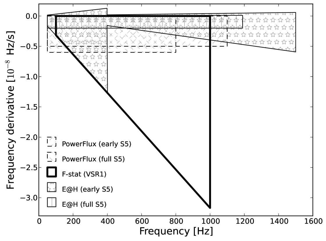
Given that the data we analyzed (Virgo VSR1) had a higher noise and the duration was shorter than the LIGO S5 data we have achieved a lower sensitivity than in the most recent E@H search [22]. However due to very good efficiency of our code we were able to analyze a much larger parameter space. We have analyzed a large part of the plane that was previously unexplored by any of the all-sky searches. For example in this analysis the plane searched was larger than that in the full S5 E@H search [22] (see Figure 5). In addition, the data from the Virgo detector is characterized by different spectral artifacts (instrumental and environmental) from these seen in LIGO data. As a results, certain narrow bands excluded from LIGO searches because of highly non-Gaussian noise can be explored in this analysis.
The paper is organized as follows. In Section 2 we describe the data from the Virgo detector VSR1 run, in Section 3 we explain how the data were selected. In Section 4 the response of the detector to a gravitational wave signal from a rotating neutron star is briefly recalled. In Section 5 we introduce the -statistic. In Section 6 we describe the search method and present the algorithms for an efficient calculation of the -statistic. In Section 7 we describe the vetoing procedure of the candidates. In Section 8 we present the coincidence algorithm that is used for post-processing of the candidates. Section 9 contains results of the analysis. In Section 10 we determine the sensitivity of this search, and we conclude the paper by Section 11. In A we present a general formula for probability that is used in the estimation of significance of the coincidences.
2 Data from the Virgo’s first science run
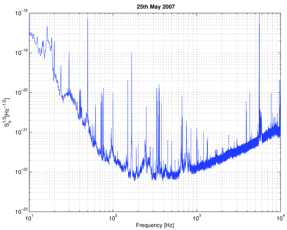
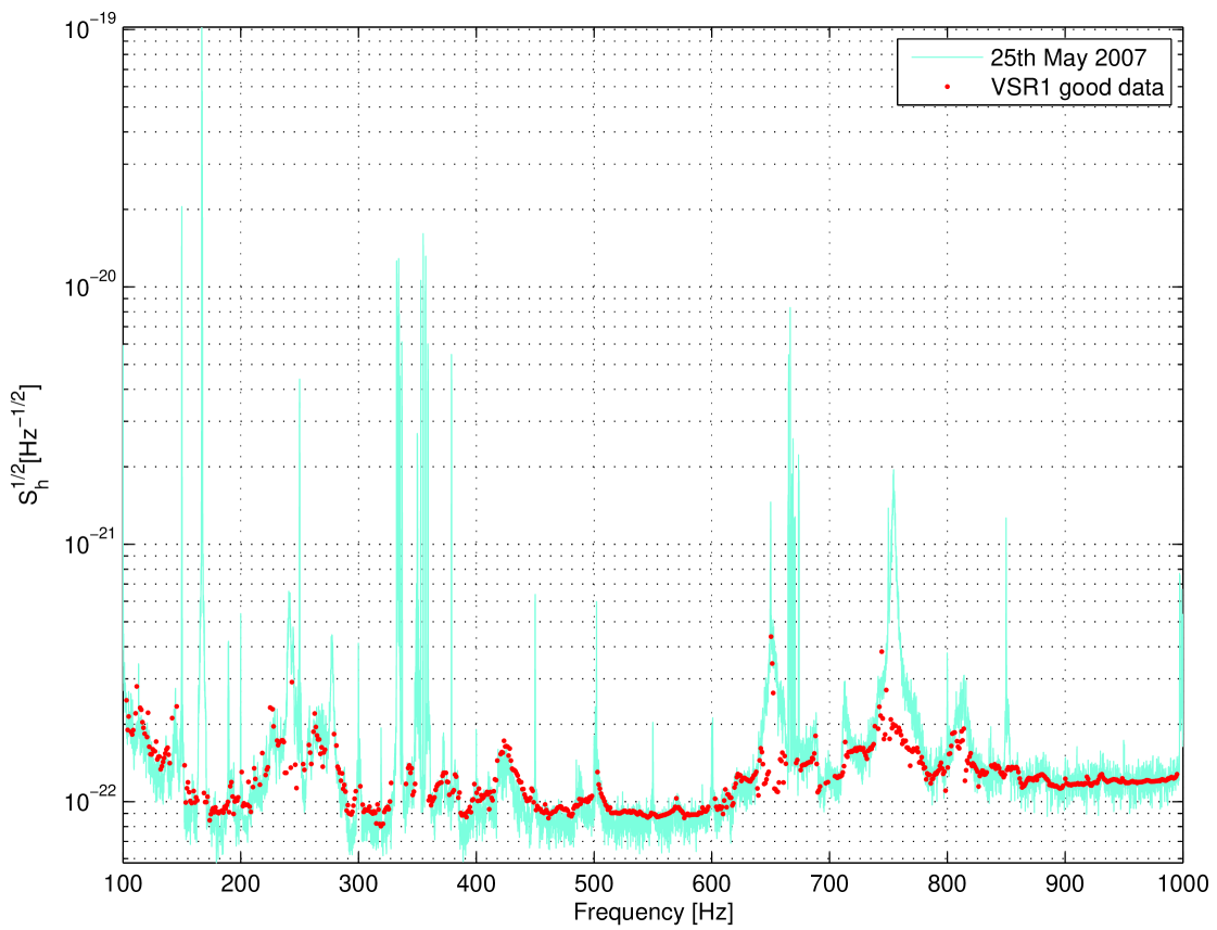
The VSR1 science run spanned more than four months of data acquisition. This run started on May 18, 2007 at 21:00 UTC and ended on October 1, 2007 at 05:00 UTC. The detector was running close to its design sensitivity with a duty cycle of 81.0% [23]. The data were calibrated, and the time series of the gravitational wave strain was reconstructed. In the range of frequencies from 10Hz to 10kHz the systematic error in amplitude was 6% and the phase error was 70 mrad below the frequency of 1.9 kHz [24]. A snapshot of the amplitude spectral density of VSR1 data in the Virgo detector band is presented in Figure 1.
3 Data selection
The analysis input consists of narrow-band time-domain data segments. In order to obtain these sequences from VSR1 data, we have used the software described in [25], and extracted the segments from the Short Fourier Transform Database (SFDB). The time domain data sequences were extracted with a certain sampling time , time duration and offset frequency . Thus each time domain sequence has the band , where . We choose the segment duration to be exactly two sidereal days and the sampling time equal to s, i.e., the bandwidth Hz. As a result each narrow band time segment contains data points. We have considered 67 two-day time frames for the analysis. The starting time of the analysis (the time of the first sample of the data in the first time frame) was May 19, 2007 at 00:00 UTC. The data in each time frame were divided into narrow band sequences of 1Hz band each. The bands overlap by Hz resulting in 929 bands numbered from 0 to 928. The relation between the band number and the offset frequency is thus given by
| (1) |
Consequently, we have 62 243 narrow band data segments. From this set we selected good data using the following conditions. Let be the number of zeros in a given data segment (data point set to zero means that at that time there was no science data). Let be the band of a given data segment. Let and be the minimum and the maximum of the amplitude spectral density in the interval . Spectral density was estimated by dividing the data of a given segment into short stretches and averaging spectra of all the short stretches. We consider the data segment as good data and use it in this analysis, if the following two criteria are met:
-
1.
,
-
2.
.
20 419 data segments met the above two criteria. Figure 2 shows a time-frequency distribution of the good data segments.
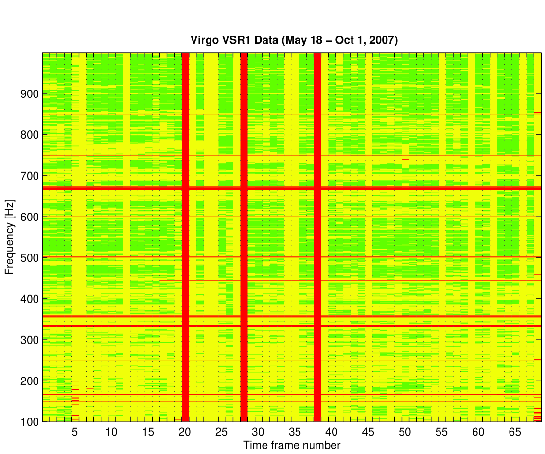
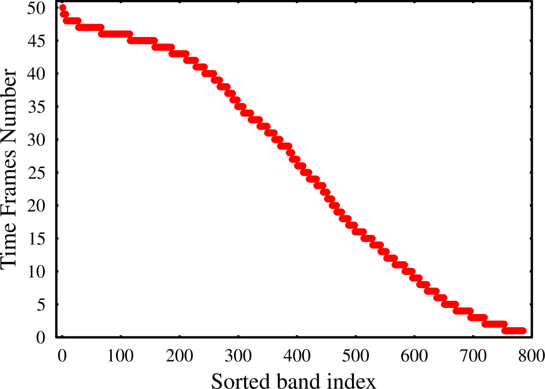
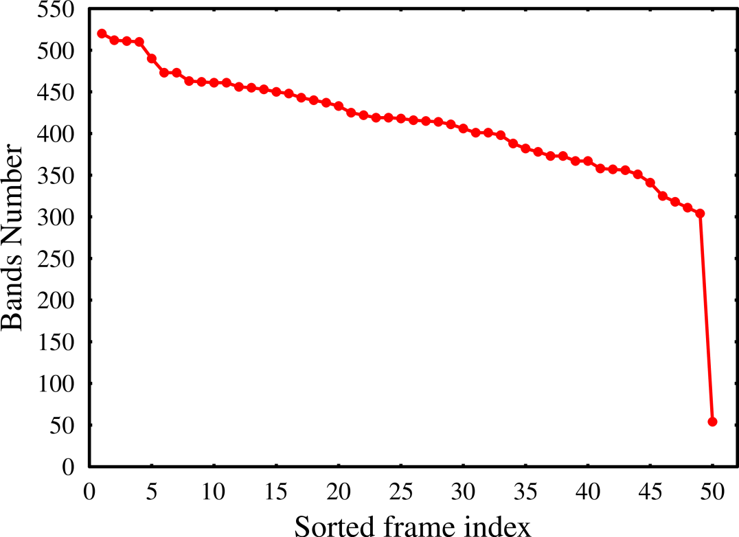
The good data appeared in 50 out of 67 two-day time frames and in 785 out of 929 bands. The distribution of good data segments in time frames and in bands is given in Figure 3.
In Figure 4 we plot a snapshot spectral density of VSR1 data presented in Figure 1 and an estimate of the spectral density of the data that was used in the analysis. We estimate the spectral density in each band by a harmonic mean of the spectral densities of each of the two-day time segments chosen for the analysis in the band. As the data spectrum in each band is approximately white, we estimate the spectral density in each time segment by , where is the variance of the data in a segment and is the s sampling time. We plot the band from 100Hz to 1 kHz which we have chosen for this search.
4 The response of the detector
The dimensionless noise-free response of a gravitational-wave detector to a weak plane gravitational wave in the long wavelength approximation, i.e., when the characteristic size of the detector is much smaller than the reduced wavelength of the wave, can be written as the linear combination of the two independent wave polarizations and ,
| (2) |
where and are the detector’s beam-pattern functions,
| (3) | |||
| (4) |
The beam-patterns and are linear combinations of and , where is the polarization angle of the wave. The functions and are the amplitude modulation functions, that depend on the location and orientation of the detector on the Earth and on the position of the gravitational-wave source in the sky, described in the equatorial coordinate system by the right ascension and the declination angles. They are periodic functions of time with the period of one and two sidereal days. The analytic form of the functions and for the case of interferometric detectors is given by Eqs. (12) and (13) of [18]. For a rotating nonaxisymmetric neutron star, the wave polarization functions are of the form
| (5) |
where and are constant amplitudes of the two polarizations and is the phase of the wave, being the initial phase of the waveform. The amplitudes and depend on the physical mechanism responsible for the gravitational radiation, e.g., if a neutron star is a triaxial ellipsoid rotating around a principal axis with frequency , then these amplitudes are
| (6) |
where is the angle between the star’s angular momentum vector and the direction from the star to the Earth, and the amplitude is given by
| (7) |
Here is the star’s moment of inertia with respect to the rotation axis, is the distance to the star, and is the star’s ellipticity defined by , where and are moments of inertia with respect to the principal axes orthogonal to the rotation axis. We assume that the gravitational waveform given by Eqs. (2)–(5) is almost monochromatic around some angular frequency , which we define as instantaneous angular frequency evaluated at the solar system barycenter (SSB) at , and we assume that the frequency evolution is accurately described by one spindown parameter . Then the phase is given by
| (8) |
where, neglecting the relativistic effects, is the vector that joins the SSB with the detector, and is the unit vector pointing from SSB to the source. In equatorial coordinates , we have .
5 The - statistic
A method to search for gravitational wave signals from a rotating neutron star in a detector data uses the -statistic, described in [18]. The -statistic is obtained by maximizing the likelihood function with respect to the four unknown parameters - , , , and . This leaves a function of only the remaining four parameters - , , , and . Thus the dimension of the parameter space that we need to search decreases from 8 to 4. In this analysis we shall use an observation time equal to the integer multiple of sidereal days. Since the bandwidth of the signal over our coherent observation time of two days is very small, we can assume that over this band the spectral density of the noise is white (constant). Under these assumptions the -statistic is given by [26, 27]
| (9) |
where is the variance of the data, and
| (10) | |||
| (11) |
6 Description of the search
The search consists of two parts; the first part is a coherent search of two-day data segments, where we search a 4-parameter space defined by angular frequency , angular frequency derivative , declination , and right ascension . The search is performed on a 4-dimensional grid in the parameter space described in Section 6.2. We set a fixed threshold of 20 for the -statistic for each data segment. This corresponds to a threshold of 6 for the signal-to-noise ratio. All the threshold crossings are recorded together with corresponding 4 parameters of the grid point and the signal-to-noise ratio . The signal-to-noise is calculated from the value of the -statistic at the threshold crossing as
| (12) |
In this way for each narrow band segment we obtain a set of candidates. The candidates are then subject to the vetoing procedure described in Section 7. The second part of the search is the post-processing stage involving search for coincidences among the candidates. The coincidence procedure is described in Section 8.
6.1 Choice of the parameter space
We have searched the frequency band from 100 Hz to 1 kHz over the entire sky. We have followed [13] to constrain the maximum value of the parameter for a given frequency by , where is the minimum spindown age111The factor of two in this formula appears here because the spindown parameter used in [13] is twice the spindown parameter used in this work.. We have chosen yr for the whole frequency band searched. Also, in this search we have considered only the negative values for the parameter , thus assuming that the rotating neutron star is spinning down. This gives the frequency-dependent range of the spindown parameter where :
| (13) |
We have considered only one frequency derivative. Estimates taking into account parameter correlations (see [13] Figure 6 and Eqs. (6.2) - (6.6)) show that even for the minimum spindown age of yr and for two days coherent observation time that we consider here, it is sufficient to include just one spindown parameter.
In Figure 5 we have compared the parameter space searched in this analysis in the plane with that of other recently published all-sky searches: Einstein@Home early S5 search [21], Einstein@Home full S5 [22], PowerFlux early S5 [28], PowerFlux full S5 [17].
6.2 Efficient calculation of the -statistic on the grid in the parameter space
Calculation of the -statistic (Eq. (9)) involves two sums given by Eqs. (10). By introducing a new time variable called the barycentric time ([29, 18, 27])
| (14) |
we can write these sums as discrete Fourier transforms in the following way
| (15) | |||
where
| (16) |
Written in this form, the two sums can be evaluated using the Fast Fourier Transform (FFT) algorithm thus speeding up their computation dramatically. The time transformation described by equation (14) is called resampling. In addition to the use of the FFT algorithm we apply an interpolation of the FFT using the interbinning procedure (see [27] Section VB). This results in the -statistic sampled twice as fine with respect to the standard FFT. This procedure is much faster than the interpolation of the FFT obtained by padding the data with zeroes and calculating a FFT that is twice as long. With the approximations described above for each value of the parameters , , and , we calculate the -statistic efficiently for all the frequency bins in the data segment of bandwidth 1Hz.
In order to search the 4-dimensional parameter space, we need to construct a 4-dimensional grid. To minimize the computational cost we construct a grid that has the smallest number of points for a certain assumed minimal match [30]. This problem is equivalent to the covering problem [31, 32] and it has the optimal solution in 4-dimensions in the case of a lattice i.e., a uniformly spaced grid. In order that our parameter space is a lattice, the signals’ reduced Fisher matrix must have components that are independent of the values of the parameters. This is not the case for the signal given by Eqs. (2) - (8); it can be realized however for an approximate signal called the linear model described in Section IIIB of [27]. The linear model consists of neglecting amplitude modulation of the signal and discarding the component of the vector joining the detector and the solar system barycenter that is perpendicular to the ecliptic. This approximation is justified because the amplitude modulation is very slow compared to the phase modulation and the discarded component in the phase is small compared to the others. As a result the linear model signal has a constant amplitude , and one can find parameters such that the phases are linear functions of them. We explicitly have (see Section IIIB of [27] for details):
| (17) |
where
| (18) |
The parameters and are defined by
| (19) | |||
| (20) |
where is the obliquity of the ecliptic, and and are known functions of the detector ephemeris.
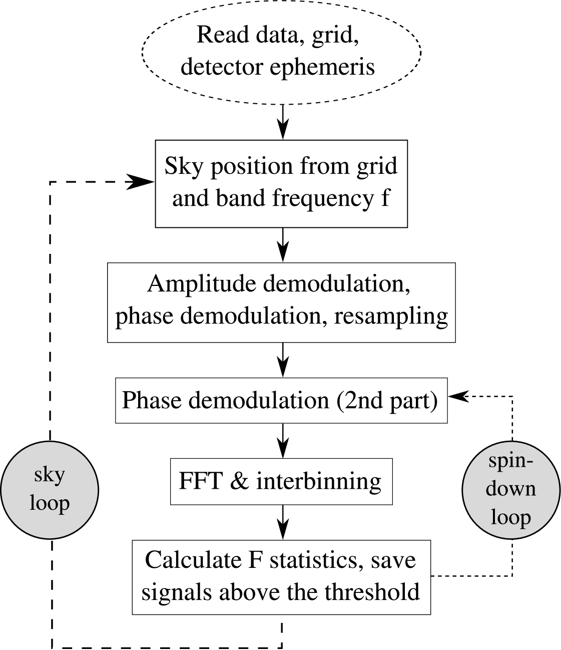
In order that the grid is compatible with application of the FFT, its points should be constrained to coincide with Fourier frequencies at which the FFT is calculated. Moreover, we observed that a numerically accurate implementation of the interpolation to the barycentric time (see Eq. (14)) is so computationally demanding that it may offset the advantage of the FFT. Therefore we introduced another constraint in the grid such that the resampling is needed only once per sky position for all the spindown values. Construction of the constrained grid is described in detail in Section IV of [27]. In this search we have chosen the value of the minimal match . The workflow of the coherent part of the search procedure is presented in Figure 6.
7 Vetoing procedure
We apply three vetoing criteria to the candidates obtained in the coherent part of the search - line width veto, stationary line veto and polar caps veto. Data from the detector always contain some periodic interferences (lines) that are detector artifacts. An important part of our vetoing procedure was to identify the lines in the data. We have therefore performed a Fourier search with frequency resolution of 1/(2 days) Hz for periodic signals of each of the two-day data segments. We compared the frequencies of the significant periodic signals identified by our analysis with the line frequencies obtained by the Virgo LineMonitor and we found that all the lines from the LineMonitor were detected by our Fourier search.
7.1 Line width veto
We veto all the candidates with frequency around every known line frequency according to the following criterion
| (21) |
where the width is estimated as
| (22) |
where is the maximum value of the velocity of the detector with respect to the SSB during the observation time, is the maximum distance to the SSB during the coherent observation time , and is the maximum of the absolute value of the frequency derivative. Eq. (22) determines the maximum smearing of the frequency on each side of the line due to frequency modulation induced by the filters applied in the -statistic.
7.2 Stationary line veto
Let us consider the instantaneous frequency of the signal, i.e., the time derivative of the phase:
| (23) |
where . The frequency derivative of the instantaneous frequency is given by
| (24) |
where . Eq. (24) is the rate of change of detector response frequency for a source whose SSB frequency and spindown are and . An instrumental line has a constant detector frequency and mimics a source for which the r.h.s of Eq. (24) vanishes. In practice, we veto candidates with
| (25) |
for some . In the search we choose , where is the observation time. The above stationary line veto was introduced in reference [14] and refined in [33]; it was used in the first two E@H searches [20, 21].
7.3 Polar caps veto
We observe that many of the detected lines cluster around the poles where declination is close to . An interference originating from a detector will correlate well with our templates if the frequency modulation in Eq. (23) is minimized. Assuming that and that the diurnal motion of the Earth averages to 0 over two days observation time, this happens when the quantity is minimized. We find that this quantity is close to minimum independently of the value of when . Thus we veto candidates that are too close to the poles; we discard all candidates with the declination angle within three grid cells from the poles.
8 Coincidences
In order to find coincidences among the candidates, we applied a method similar to the one used in the first two E@H searches [20, 21]. For each band we have searched for coincidences among candidates in different time frames. We are able to search for coincidences only in those bands where there were two or more time frames with data selected for the analysis. If we search for a real gravitational wave signal, we must take into account frequency evolution due to spindown of the rotating neutron star. Thus the first step in the coincidence analysis was to transform all frequencies of the candidates to a common fiducial reference time . We have chosen the fiducial time to be the time of the first sample of the latest time frame that we analyzed i.e., the 67th time frame. We have
| (26) |
where is the time of the first sample of the th time frame. The next step was to divide the parameter space into cells. This construction of the coincidence cell was different from that in the E@H analysis. To construct the cells in the parameter space we have used the reduced Fisher matrix for the linear signal model defined by Eqs. (17) and (18). The reduced Fisher matrix is the projected Fisher matrix on the 4-dimensional space spanned by parameters . We define the cell in the parameter space by the condition:
| (27) |
Because the ephemeris of the detector is different in each of the time frames, the reduced Fisher matrix is different in each time frame. To have a common coincidence grid we have chosen the grid defined by the latest frame i.e., the frame no. 67 as the coincidence grid. After the transformation of the candidate frequencies to a reference time and construction of the coincidence grid, the coincidence algorithm for each of the bands proceeded in the following steps:
-
1.
Transform angles and to and coordinates (see Eq.(19))
-
2.
Transform candidate parameters to coordinates defined by
(28) where are eigenvectors of the matrix , and are its eigenvalues. In these coordinates the Fisher matrix is proportional to the unit matrix.
-
3.
Coordinates are rounded to the nearest integer. In this way we sort candidates efficiently into adjacent 4-dimensional hypercubes. If there are more than one candidates from a given data segment in a hypercube we select the candidate that has the highest SNR. We do sorting for each time frame in the band. If there is more than one candidate in a given hypercube we register a coincidence.
-
4.
We shift cubes by 1/2 of their size in all possible directions, and for each shift we search for coincidences.
This last step of the algorithm takes into account cases for which the candidate events are located on opposite sides of cell borders, edges, and corners and consequently coincidences that could not be found just by packing candidates into adjacent cells.
The most significant coincidence in each band is the one which has the highest multiplicity. For each most significant coincidence we have calculated the false alarm probability i.e., the probability that such a coincidence can occur purely by chance. The false alarm probability is calculated using the formula explained in A and given by Eq. (35). This general formula applies to a variable number of candidates in various time slots and also takes into account the shifts of the cells in the parameter space.
9 The search
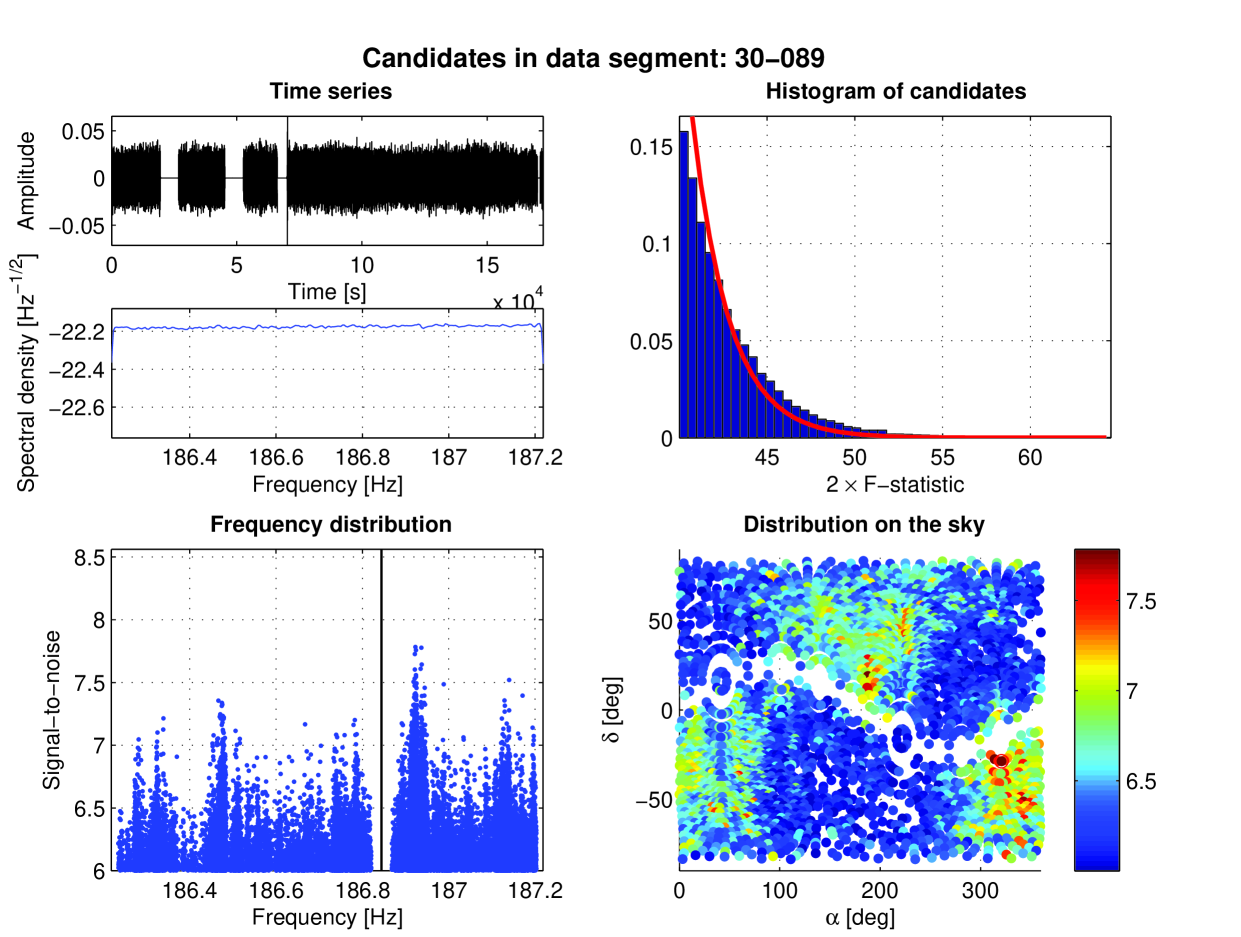
In this analysis we have searched coherently 20 419 two-day time segments of data narrowbanded to Hz. In the coherent part of the search described in Section 6 we have used templates which is the number of -statistic values computed. This resulted in 20 419 candidate files containing candidates. The candidates were subject to the vetoing using the three veto criteria: line veto, polar caps veto, and stationary line veto described in Section 7. As a result of vetoing around 24% of the candidates were discarded leaving candidates. Nearly all candidates were vetoed by the line veto, whereas 0.20% were vetoed by the stationary line criterion and only % by the polar caps veto. In Figure 7 we present an example of the candidate distribution obtained from the coherent search of one narrow band data segment and after the vetoing procedure.
In the next step we have searched for the significant coincidences among the candidates. We have searched for coincidences in all the frequency bands where there were two or more data segments analyzed. In Figure 8 we have plotted the highest coincidence multiplicity for each of the bands. The highest multiplicity was 6, and it occurred in 10 bands. The multiplicity tends to grow with the frequency, because the size of the parameter space grows as .
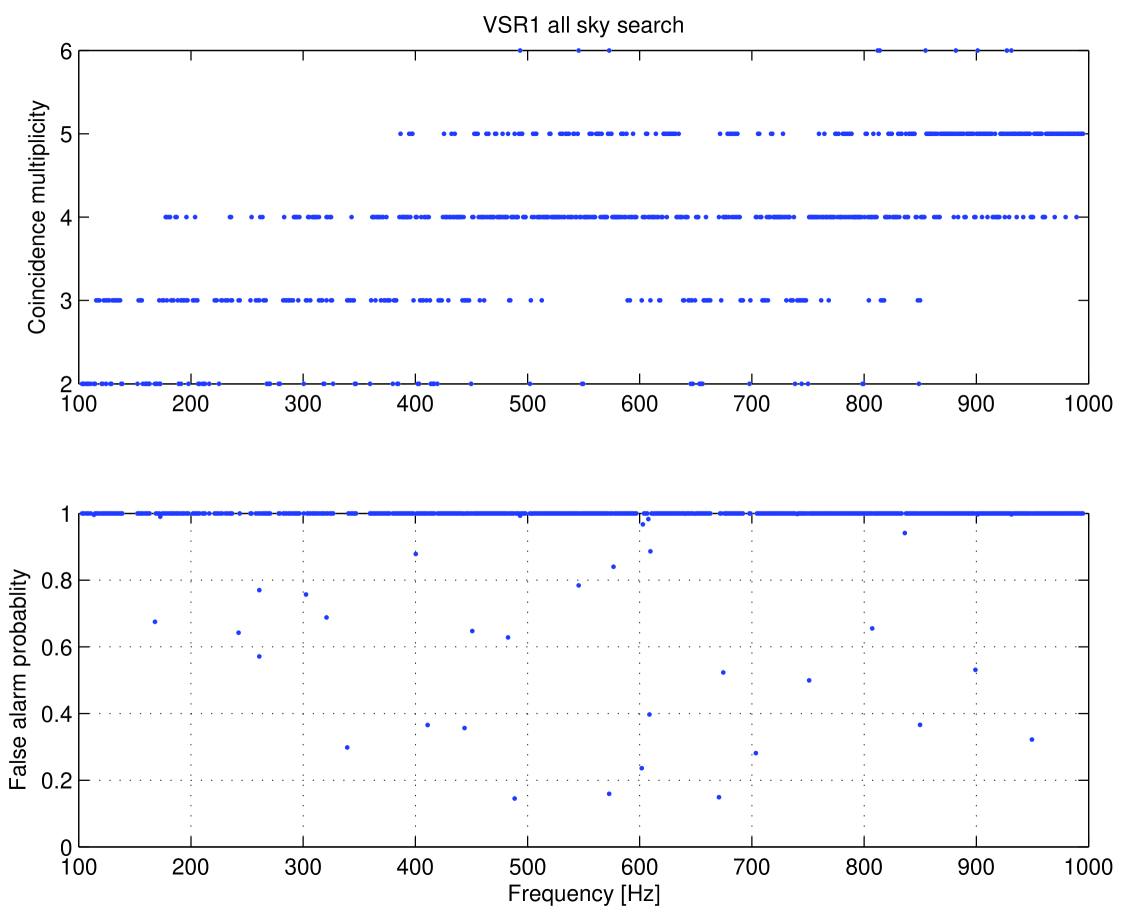
For each band we have calculated the false alarm probability corresponding to the most significant coincidence using Eq. (35). The most significant coincidence occurred in band no. 401, corresponding to the frequency range of Hz. It was a coincidence of multiplicity = 5, and its false alarm probability was 14.5%. Note that a coincidence with the highest multiplicity is not the most significant. This is because the significance depends on the number of time frames with candidates in a given band and also on the number of candidates in the time frames. By adopting a criterion used by E@H searches that the background coincidences correspond to false alarm probability of 0.1% or greater, we conclude that we have found no significant coincidence and thus no viable gravitational wave candidate. Considering the significance of the coincidences, we could adopt even a 10% false alarm probability as a background. Consequently, we proceed to the final stage of our analysis - estimation of sensitivity of the search.
10 Sensitivity of the search
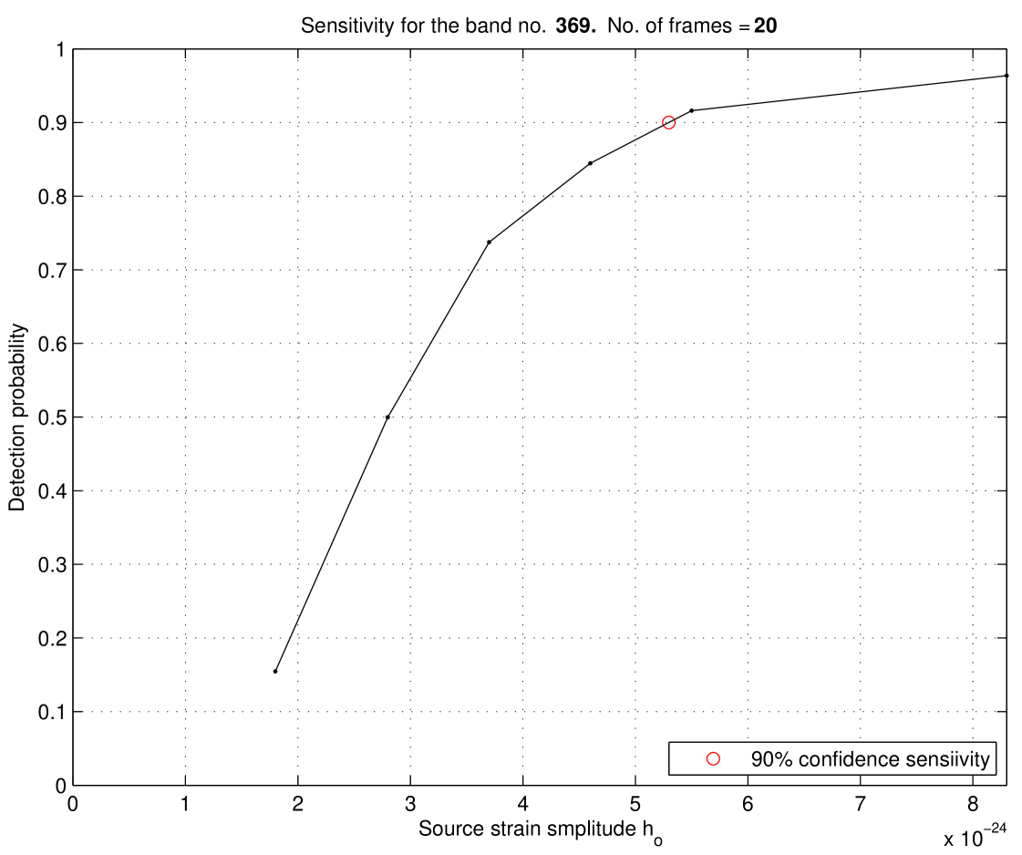
The sensitivity of the search is taken to be the amplitude of the gravitational wave signal that can be confidently detected. To estimate the sensitivity we use a procedure developed in [20]. We determine the sensitivity of the search in each of the 785 frequency bands that we have searched. To determine the sensitivity, we perform Monte Carlo simulations in which, for a given amplitude , we randomly select the other seven parameters of the signal: and . We choose frequency and spindown parameters uniformly over their range, and source positions uniformly over the sky. We choose angles and uniformly over the interval and we choose uniformly over the interval . For each band we add the signal to all the data segments chosen for the analysis in that band. Then we process the data through our pipeline. First, we perform a coherent -statistic search of each of the data segments where the signal was added, and store all the candidates above our -statistic threshold of 20. In this coherent analysis, to make the computation manageable, we search over only parameter space consisting of 2 grid points around the nearest grid point where the signal was added. Then we apply our vetoing procedure to the candidates obtained as explained in Section 7. Finally, we perform coincidence analysis of the candidates that survive vetoing which is described in Section 8. We define a detectable signal if it is coincident in more than 70% of the time frames in a given band. This condition is similar to the condition used in the two E@H searches, where a coincidence method was used [20, 21]. For bands with only one frame available the coherent search over one -day data segment was performed. In this case the injected signal is declared detected if its signal-to-noise ratio obtained in the coherent search is larger than the signal-to-noise ratio of the loudest signal in that data segment without an injection. For each band we inject signals with 5 different amplitude values, and perform 100 randomized injections for each amplitude. For each amplitude we calculate how many signals were detected, and by interpolation we determine the amplitude corresponding to 90% of signals detected. This amplitude was defined as the 90% confidence sensitivity. Sometimes even for the highest amplitude we have not reached the detection probability. In this case we performed injections for higher amplitudes until the desired level of detectability was achieved. In Figure 9, as an example, we present an estimation of the sensitivity in the band corresponding to the frequency range of Hz. The errors in the sensitivity estimates originate from calibration errors in the amplitude and errors due to a finite number of Monte Carlo injections. We use 100 injections; hence from a binomial statistic, one is equivalent to 3% fluctuation. Thus the estimated amplitude sensitivity corresponds to confidence in the range from 87% to 93%. To estimate how this uncertainty in confidence translates into uncertainty in the amplitude we have performed an additional set of injections for a range of amplitudes close to the estimated sensitivity and from the slope of the confidence vs. amplitude we determined the uncertainty in the amplitude. To increase the accuracy of the error estimate, we have performed 1000 injections for each amplitude. The uncertainty in the amplitude was not more than 5%. The calibration errors in VSR1 data are 6% (see Section 2). Adding these two types of errors in quadrature results in the total error in sensitivity estimate to be around 7%.
The sensitivity of this search obtained through Monte Carlo simulations for the whole band searched is presented in Figure 10.
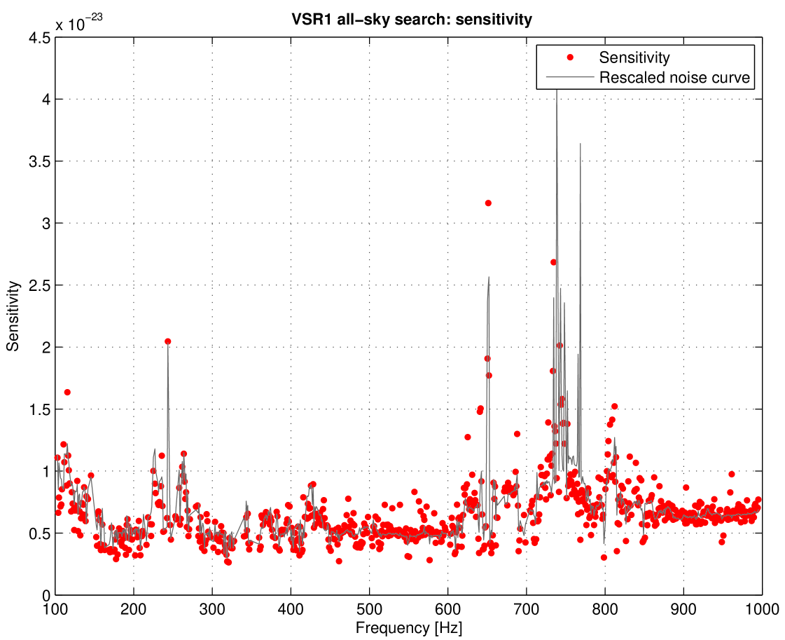
We see from Figure 10 that the sensitivity essentially reflects the instrumental noise curve given in Figure 4. We have made a fit of the sensitivity to the one-sided spectral density of detector noise described by the following relation:
| (29) |
We find that the prefactor is in the range from 15.6 to 22.4 and it depends on the frequency band and the number of the data segments in the band.
11 Conclusions
The sensitivity of this search was 50% to 2 times better, depending on the bandwidth, than that of the LIGO S4 search [20] and comparable to the sensitivities obtained in the early LIGO S5 data [21], but to times worse than the upper limits in the E@H full LIGO S5 data search [22]. This was due to the lower noise and longer observation time for the LIGO S5 data w.r.t the Virgo VSR1 data. However, for the first time in an all-sky search we have estimated the sensitivity in the frequency band from 400Hz to 1kHz and the frequency spindown range from Hz/s to Hz/s, which is a previously unexplored region in the parameter space.
The next step is to test the search method described in this paper in the Mock Data Challenge (MDC) designed by the LIGO and Virgo projects to validate and compare pipelines that are proposed to be used in the analysis of the forthcoming data from the advanced detectors. It is also planned to further test the pipeline presented here with other data sets collected by the LIGO and Virgo detectors.
References
References
- [1] T Accadia et al 2012 JINST 7 P03012
- [2] B Abbott et al 2007 Phys. Rev. D76 082001
- [3] A Mastrano, P D Lasky and A Melatos 2013 (Preprint 1306.4503)
- [4] B J Owen 2010 Phys. Rev. D 82 104002
- [5] D J Jones and N Andersson 2001 Mon. Not. R. Astron. Soc. 331 203
- [6] L Bildsten 1998 Astrophys. J. 501 L89
- [7] G Ushomirsky, C Cutler and L Bildsten 2000 Mon. Not. R. Astron. Soc. 319 902
- [8] C Cutler 2002 Phys. Rev. D 66 084025
- [9] A Melatos and D J B Payne 2005 Astrophys. J. 623 1044
- [10] B J Owen 2005 Phys. Rev. Lett. 95 211101
- [11] N K Johnson-McDaniel and B J Owen 2013 Phys. Rev. D 88 044004
- [12] C J Horowitz and K Kadau 2009 Phys. Rev. Lett. 102 191102
- [13] P R Brady, T Creighton, C Cutler and B F Schutz 1998 Phys. Rev. D 57 2101
- [14] B Abbott et al 2008 Phys. Rev. D77 022001
- [15] B Abbott et al 2005 Phys. Rev. D 72 102004
- [16] B Abbott et al 2009 Phys. Rev. Lett. 102 111102
- [17] J Abadie et al 2012 Phys. Rev. D85 022001
- [18] P Jaranowski, A Królak and B Schutz 1998 Phys. Rev. D 58 063001
- [19] http://einstein.phys.uwm.edu
- [20] B Abbott et al 2009 Phys. Rev. D79 022001
- [21] B Abbott et al 2009 Phys. Rev. D80 042003
- [22] J Aasi et al 2013 Phys. Rev. D87 042001
- [23] F Acernese et al 2008 Class. Quant. Grav. 25 184001
- [24] T Accadia et al 2010 Journal of Physics: Conference Series 228 012015
- [25] P Astone et al 2002 Phys. Rev. D 65 022001
- [26] P Astone, K M Borkowski, P Jaranowski and A Królak 2002 Phys. Rev. D 65 042003
- [27] P Astone, K M Borkowski, P Jaranowski, M Pietka and A Królak 2010 Phys. Rev. D 82 022005
- [28] B Abbott et al 2009 Phys. Rev. Lett. 102 111102
- [29] B F Schutz The Detection of Gravitational Waves ed Blair D (Cambridge University Press)
- [30] B Owen 1996 Phys. Rev. D 53 6749
- [31] J H Conway and N J A Slone 1999 Sphere packings, lattices and groups (New York: Springer)
- [32] Prix R 2007 Phys. Rev. D 75 023004
- [33] H J Pletsch 2008 Phys. Rev. D 78 102005
Appendix A False alarm coincidence probability
Let us assume that for a given frequency band we analyze non-overlapping time segments. Suppose that the search of the th segment produces candidates. Let us assume that the size of the parameter space for each time segment is the same, and it can be divided into the number of independent cells. We would like to test the null hypothesis that coincidences among candidates from segments are accidental. The probability for a candidate event to fall into any given coincidence cell is equal to . Thus probability that a given coincidence cell is populated with one or more candidate events is given by
| (30) |
We may also consider independent candidates only, i.e., such that there is no more than one candidate within one cell. If we obtain more than one candidate within a given cell we choose the one which has the highest signal-to-noise ratio. In this case
| (31) |
The probability that any given coincidence cell out of the total of cells contains candidate events from or more distinct data segments is given by a generalized binomial distribution
| (32) | |||||
where is the sum over all the permutations of the data sequences. Finally the probability that there is or more coincidences in one or more of the cells is
| (33) |
The above formula for the false alarm coincidence probability does not take into account the case when candidate events are located on opposite sides of cell borders, edges, and corners. In order to find these coincidences the entire cell coincidence grid is shifted by half a cell width in all possible combinations of the four parameter-space dimensions, and coincidences are searched in all the 16 coincidence grids. This leads to a higher number of accidental coincidences, and consequently Eq. 33 underestimates the false alarm probability. Let us consider the simplest one-dimensional case. In this case we have possible shifts (the original coincidence grid and the one shifted by half). This increases probability by a factor of if the two cell coincidence grids were independent. However the cells overlap by half and some coincidences would be counted twice. To account for this we divide the cells in the coincidence grid by half resulting in cells and define the false alarm probability that any given half of the coincidence cell out of the total of half cells contains candidate events from or more distinct data segments. These are coincidences that were already counted, and consequently the false alarm probability with the cell shift is . This results in the false alarm probability
| (34) |
To generalize the above formula to higher dimensions we need to consider further shifts and divisions of the cells. In the four dimension case this leads to the formula for the probability that there are or more independent coincidences in one or more of the cells in all 16 grid shifts given by
| (35) | |||
By choosing a certain false alarm probability , we can calculate the threshold number of coincidences. If we obtain more than coincidences in our search we reject the null hypothesis that coincidences are accidental only at the significance level of .