Implementing arbitrary quantum operations via quantum walks on a cycle graph
Abstract
The quantum circuit model is the most commonly used model for implementing quantum computers and quantum neural networks whose essential tasks are to realize certain unitary operations. The circuit model usually implements a desired unitary operation by a sequence of single-qubit and two-qubit unitary gates from a universal set. Although this certainly facilitates the experimentalists as they only need to prepare several different kinds of universal gates, the number of gates required to implement an arbitrary desired unitary operation is usually large. Hence the efficiency in terms of the circuit depth or running time is not guaranteed. Here we propose an alternative approach; we use a simple discrete-time quantum walk (DTQW) on a cycle graph to model an arbitrary unitary operation without the need to decompose it into a sequence of gates of smaller sizes. Our model is essentially a quantum neural network based on DTQW. Firstly, it is universal as we show that any unitary operation can be realized via an appropriate choice of coin operators. Secondly, our DTQW-based neural network can be updated efficiently via a learning algorithm, i.e., a modified stochastic gradient descent algorithm adapted to our network. By training this network, one can promisingly find approximations to arbitrary desired unitary operations. With an additional measurement on the output, the DTQW-based neural network can also implement general measurements described by positive-operator-valued measures (POVMs). We show its capacity in implementing arbitrary 2-outcome POVM measurements via numeric simulation. We further demonstrate that the network can be simplified and can overcome device noises during the training so that it becomes more friendly for laboratory implementations. Our work shows the capability of the DTQW-based neural network in quantum computation and its potential in laboratory implementations.
I introduction
Quantum walk Aharonov , the quantum counterpart of classical random walk, has been widely applied in achieving various quantum information processing tasks Portugal . Because of its quadratic enhancement of variances, the quantum walk plays a vital role in many quantum search algorithms and provides possible exponential speedups due to the quantum interference during the walk Kempe . Moreover, various experimental implementations of quantum walks prove its feasibility in real-life circumstances of quantum information processing Kia .
On the other hand, machine learning is a core technology in the age of artificial intelligence. Since machine learning faces the challenge of the lack of computational power and quantum computing has a vast computational potential, the possibility of combining quantum computing and machine learning has been considered. Quantum neural networks (QNNs), a newer class of models in the field of quantum machine learning, operate on quantum computers and perform calculations using quantum effects like superposition, entanglement, and interference. Investigations on QNNs farhi2018classification ; zhao2019building ; mitarai2018quantum ; dallaire2018quantum ; amin2018quantum ; CZoufal ; VDunjko ; MSchuld have revealed their potential advantages, such as training and processing speedups. Despite significant developments in the growing field of quantum machine learning, the trade-offs between quantum and classical models have not been systematically studied. In particular, the question of whether quantum neural networks are more powerful than classical neural networks is still open SAaronson2015nph .
A gate-model QNN is a QNN constructed on a gate-model quantum computer using a sequence of unitaries with associated gate parameters farhi2018classification . Recent developments, such as quantum generative adversarial networks and quantum circuit learning, have more general and diverse QNN structures dallaire2018quantum ; mitarai2018quantum ; gyongyosi2019training . Researchers have already proved that typical quantum walks are universal for quantum computation childs2009universal ; lovett2010universal ; kurzynski2013quantum ; bian2015realization ; zhao2015experimental . However, these works mainly focus on state processing, and many auxiliary systems should be employed in general. In contrast, what we are attempting to achieve in this work is a universal control of the quantum system to implement arbitrary quantum operations, without any auxiliary system. For this purpose, we shall introduce a QNN based on discrete-time quantum walks (DTQW) on a cycle graph with specifically parameterized coin operators. We choose the graph to be a cycle because it is simple for laboratory implementations. We will prove that the DTQW-based QNN is indeed capable of realizing arbitrary unitary evolution of the closed system.
Determining the parameters of the DTQW-based QNN analytically is possible. However, any further adjustments on the network, such as a reduction in the number of circuit depth, will pose extraordinary difficulties for analytical methods. In contrast, we will show that such adjustments can be effectively made with gradient descent, a well-known optimization algorithm frequently employed to train machine learning models, including both classical and quantum neural networks darken1992learning ; bengio2013advances . Another significant advantage of using gradient descent is that explicitly decomposing the desired operator into a sequence of gates from a universal set is no longer necessary. Furthermore, we shall simplify the network in various ways to facilitate laboratory implementations. For example, we shall use only rotations along the x-axis as the gates involved in the DTQW. We can still find decent approximations of the desired quantum operations in this situation using our DTQW-based QNN.
Our work is organized as follows. We first introduce our DTQW-based neural network in Sec. II and then prove its universality for quantum control in Sec. III. We further modify gradient descent and apply it to our DTQW-based QNN in Sec. IV. Finally, we simplify the QNN in Sec. V to facilitate the laboratory implementations.
II Quantum neural network based on discrete time quantum walk
The quantum neural network based on quantum gates, the gate-model QNN, was first introduced due to its high experimental feasibility farhi2018classification . The gate-model QNNs utilize a series of unitary operations in a certain order to process the quantum state. The unitary operations involve adjustable parameters. By optimizing these parameters and encoding information to the input and output states, the gate-model QNNs are sufficient to solve various learning tasks. In this section, we introduce the DTQW on a cycle graph. We choose the graph to be a cycle because it is simple for laboratory implementation. We will show that such DTQW also involves a series of adjustable unitary gates and is sufficient to learn quantum operations. Thus the DTQW on a cycle graph can be treated as a special type of the gate-model QNN.
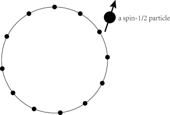
The DTQW on a cycle graph involves two Hilbert spaces, namely the coin space and the position space , which are spanned by orthonormal basis and respectively, where is the number of sites in the cycle. The walker state is then in the space . A schematic representation of the DTQW on a cycle graph is shown in Fig. 1. The process of the DTQW is an iteration of applying coin operators and shift operators
| (1) |
to the walker state, i.e.,
| (2) |
where denotes the ordinal of iterations, integer represents how far the walker is shifted if its coin is in the state . For simplicity, we choose throughout this letter. To make sure that the DTQW is flexible enough to implement various quantum operations, the coin operator need to be site-dependent, i.e.,
| (3) |
where flips the coin of the walker during the -th iteration if the walker is at the site . Since the operators are applied to the coin only if the walker is at certain sites , they are called single-site coin operators.
Since the operations during every iteration are unitary, the total effect of a -step DTQW
| (4) |
is also unitary, where denotes the time-ordered product. We define so that it is the time evolution operator, i.e., . One can notice that our version of the DTQW on a cycle graph is a straightforward generalization of the conventional Hadamard walk of which and .
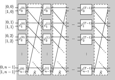
Every step of DTQW is unitary and is parameterized by . These operators can be treated as the adjustable gates in a gate-model quantum neural network. By adjusting these gates , we can use the DTQW to implement various quantum operations. Therefore the DTQW can be seen as a special type of gate-model quantum neural network. A schematic representations of the quantum neural network based on the DTQW on a cycle graph is shown in Fig. 2. The circuit depth of this network is the number of walking steps of the DTQW. In this work, we will denote the quantum neural network based on the DTQW on a cycle graph simply as the DTQW-QNN. We call the system of the quantum walker the underlying system of the DTQW-QNN.
III Universality and complexity of DTQW-based neural network
The implementation of quantum operations via the DTQW on a cycle graph is one of the primary motivations of our work. The universality of DTQW for quantum computation has been shown in general childs2009universal ; lovett2010universal . While the previous work mainly focuses on the mapping from the initial state to the final state in a certain small subspace of the total system, in this work we take the overall effect on the total system into account. In this section, we investigate the capacity and universality of the DTQW on a cycle graph in implementing quantum operations, and show that it is universal for unitary operations, which is the main theorem of this section.
By saying that the DTQW on a cycle graph is universal, we mean that any unitary operation on the overall Hilbert space can be realized by a DTQW. Hence it is not only universal for computation but also universal for controlling the whole quantum system. To be more formal and specific, the following theorem is provided.
Theorem 1.
For any unitary operator , there exists a positive integer and a family of single-site coin operators indexed by the set such that the total effect of the -step DTQW is , i.e., , as long as and .
We prove the universality of the DTQW on a cycle by decomposing arbitrary unitary operators into a product of two-level unitary operators and construct a DTQW to implement every for . A detailed proof is provided in Appendix A.
As a demonstration of Theorem 1, we first implement the controlled NOT (CNOT) gate with a DTQW on a cycle with two sites. We can find that according to Eq. (1), the shift operator
| (5) |
is just the CNOT gate we need. Hence a simple one-step DTQW is equivalent to the CNOT gate if we choose all the single-site coin operators to be the identity operator.
Next, let us consider a more complicated two-level unitary operator, a unitary controlled by two qubits
| (6) |
where are four matrix elements of . Comparing this operator with the general form of two-level operators in Eq. (17), we can find that , and . By substituting in Eqs.(26) and (27) with their respective values, we get
| (7) |
where is the Pauli matrix. By choosing the single-site coin operators according to Eq.(7), we can realize the unitary operator with an eight-step DTQW on a cycle with four sites.
For the most general two-level unitary operators , the calculation is essentially the same as the above example, i.e., find the values of by comparing with Eq. (17) and then substitute them in Eqs. (18) and (19) if or Eqs. (26) and (27) if otherwise. For unitary operators which are not two-level, we decompose them into a product of two-level unitary operators Nielsen2007Quantum . By combining the DTQWs for one after one, we can realize with the final combined DTQW. As an example, the calculation to implement the Fourier transformation is provided in Appendix B.
Implementing a unitary operation with the construction in the proof of Theorem 1 as above involves numerous steps of the walk. To reduce the number of steps, we provide in Appendix C a further optimized scheme for implementations. With this scheme, no more than steps of walk is needed for the DTQW-QNN to be universal, where is the number of sites in the cycle.
IV finding approximations via gradient descent
It is sometimes cumbersome to find exact realizations of desired quantum operations in analytical ways. However, fair approximations to desired operations are often acceptable for practical purposes. In this section, we introduce an algorithm in a machine learning fashion to find the approximations by applying gradient descent to the DTQW-QNN. With this algorithm, the required number of depth can be further reduced when approximations are allowed.
In order to apply gradient descent to the DTQW-QNN, we have to do the following three things in advance.
-
1.
Parameterize the single-site coin operators with a four dimensional real vector :
(8) in which is the th Pauli matrix, .
-
2.
Introduce a state-wise loss function :
(9) where and are the final state and the desired final state respectively.
-
3.
Derive the partial derivative:
(10) where and are the forward-propagation and back-propagation states respectively, , , and , , , equals
respectively.
Gradient descent iteratively moves the parameters in the opposite direction of the gradient, i.e.,
| (11) |
where is a positive real number called learning rate. Hence, the loss gradually drops during the iteration and the approximation to by becomes better and better.
The details of the algorithm to find the parameters of the DTQW-QNN to approximate a desired unitary operator are as the following.
-
1.
Set the total number of depth and the learning rate to be an appropriate positive integer and real respectively.
-
2.
Randomly initialize all the parameters .
-
3.
Randomly sample a state from the total Hilbert space .
-
4.
Calculate the partial derivatives for all , , according to Eq. (10).
-
5.
Update all the parameters according to Eq. (11).
- 6.
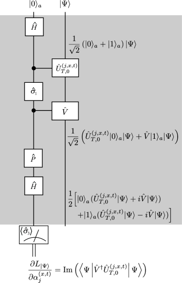
One can notice that our choice of the loss function leads to a friendly form of gradients Eq. (10) for numerical calculation. The states and can be calculated by a forward-propagation and a back-propagation efficiently. Moreover, the gradients can be calculated by implementing a circuit with the help of an ancillary qubit as shown in Fig. 3. At the last of the circuit, the average value of the ancillary qubit is measured. The result can be used to update the parameters of the DTQW-QNN since always coincides with the partial derivative in Eq. (10). This might enable us to implement simultaneous tomography and cloning of an unknown unitary operation.
Besides, the position space is commonly much larger than the coin space . Theorem 1 thus indicates that one can indirectly control a large system by controlling a small two-level coin system via DTQW on a cycle graph. For example, unitary operations and general two-outcome measurements described by positive-operator-valued measures (POVMs) can be applied to the position space in this way straightforwardly according to Theorem 1. If we are only interested in the unitary operators that act on the position space , we only need one arbitrary site to be allowed to assign nonidentity coin operators. The detailed content is provided in Appendix D.
Numerical results
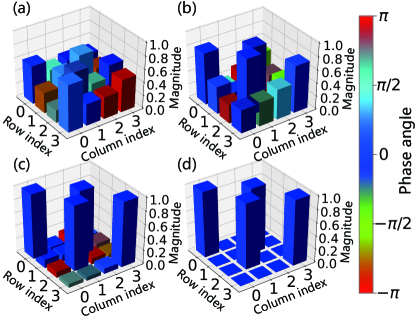
We first test our algorithm with a DTQW-QNN to learn the gate. Because all matrix elements of are either or , it would be visually clear whether a unitary operator is close to after the operator is visualized. The change of the DTQW unitary operator during the training is visualized in Fig. 4. As the DTQW-QNN is trained, becomes closer and closer to the desired gate . And the DTQW-QNN realizes the after the training is finished.
To measure how well the DTQW approximates the desired unitary , we introduce the distance
| (12) |
between the operators and . The smaller this distance is, the better the DTQW approximates the desired operator.
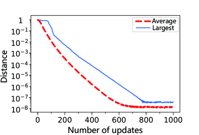
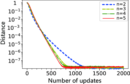
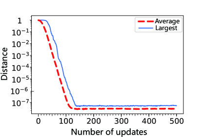
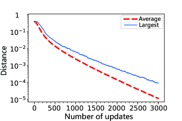
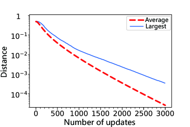
In order to show that the DTQW-QNN can actually approximate arbitrary unitary operator, we sample 200 desired operators from according to the Haar measure and train 200 DTQW-QNNs in parallel to approximate these operators respectively. The evolution of the distance during the training is plotted in Fig. 5. After the training, the final distance between the DTQW-QNN and the desired operator is smaller than even for the worst case of the 200 samples. For DTQW-QNNs with different number of sites on the cycle, Fig. 6 shows that the average distance is also always smaller than . From Fig. 6, we can also notice that with more sites on the cycle, the training of the DTQW-QNNs is faster, i.e., less updates are needed.
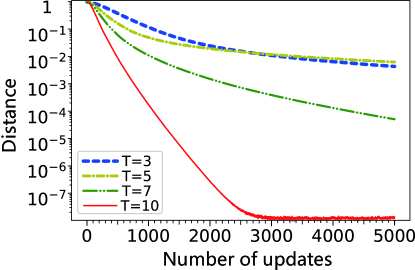
Training the DTQW-QNN exhibits some similar phenomena as training classical machine learning models. For example, the implicit acceleration by overparameterization arora2018on also emerges in the training of the DTQW-QNN. The implicit acceleration by overparameterization is a phenomenon where the neural network training becomes faster if more layers are added to the network. For DTQW-QNNs, more layers mean more steps of walk, i.e., a larger depth . As shown in Fig. 7, when the number of depth is larger, the distance drops faster during the training.
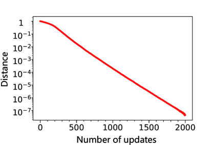
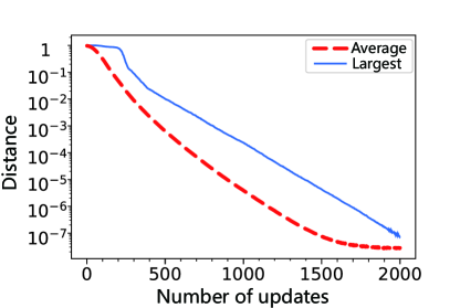
To show that the algorithm also works for larger quantum systems, we apply it to a DTQW on a cycle graph with sites as a demonstration to realize the quantum Fourier transformation. As shown in Fig. 8, this DTQW-QNN with a -dimensional underlying quantum system can still be trained to implement the operator we want. For the meta parameters used to generate the numerical results throughout this work, see Appendix E.
V Making the DTQW-based neural network more friendly for implementations
In all previous parts of this work, we have assumed that the single-site coin operators can take values from arbitrarily. This means the single-site coin operator can have arbitrary phase and arbitrary rotational axis. However, it would be much easier to implement rotations along a fixed axis with fixed phases in laboratories. Hence, in this section, we simplify the DTQW so that it becomes easier to implement. Also, there are always noises when DTQW-QNNs are implemented in laboratories. We test it under the situation where noises are presented in the single-site coin operators . Throughout this section, the numerical demonstrations are all based on DTQWs on a cycle with two sites.
V.1 Random fixed phases
Firstly, it can be observed that the phases in Eq. (8) of single-site coin operators are relative phases when are summed in Eq. (3). They are not merely a contribution to the global phase of the DTQW . Hence, any change in one of the phases may cause a nontrivial change in . This seemingly requires an annoying tuning of all the phase factors of single-site coin operators at different times and at different sites when the DTQW is implemented.
Fortunately, we find that these phase factors actually need no adjustment. As shown in Fig. 9a, the DTQW-QNN can still approximate an arbitrary operator via gradient descent even if all the phase factors signed to different sites are random and fixed during the training, i.e.,
| (13) |
where phases are independent real random variables. This releases us from the cumbersome tuning of the phases of single-site coin operators.
V.2 Simple rotations along x-axis only
The formalism of the single-site coin operators in Eq. (8) involves three consecutive rotations, namely, , each along a different axis. To make it easier for laboratory implementations, we simplify the single-site coin operators to be simple rotations only along the -axis, i.e.,
| (14) |
where now is merely a real parameter. In this situation the DTQW-QNN can still realize arbitrary operators via gradient descent, as indicated by Fig. 9b.
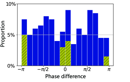
By comparing Figs. 9a and 9b, we can notice that the DTQW-QNN in this section needs much more time to train compared with the DTQW-QNN in Sec. V.1. To reveal the cause, we have trained 200 DTQW-QNNs to approximate 200 randomly sampled operators , respectively. We choose a threshold to be and mark the DTQW-QNNs of which the distance after 200 iterations of training is still larger than the threshold. We find that the phase differences of these marked DTQW-QNNs are all near or as shown in Fig. 10. Hence, we conclude that these specific differences in phases cause the DTQW-QNN to be slow to train. This result also corroborates that the phases of single-site coin operators contribute to the DTQW total effect non-trivially as we have stated in Sec. V.1. Now knowing the cause, we can easily avoid these specific phase differences when implementing DTQW-QNNs.
V.3 Noise on rotation axes
When the DTQW-QNN is implemented in laboratories, it is impossible to have all the rotation axes of be perfectly along the direction. There are always noises on the rotational axis, i.e.,
| (15) |
where
| (16) |
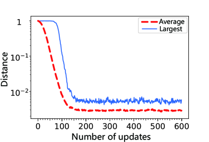
where and are independent real random variables. In this situation, approximations to desired operators still can be found via gradient descent, as shown in Fig. 11.
VI Conclusion
In conclusion, we have proposed a quantum neural network based on a simple DTQW on a cycle graph, and used the network to implement arbitrary quantum computation tasks, i.e., unitary operations on an arbitrary -dimensional Hilbert space.
In order to implement an arbitrary unitary operation via a circuit model, one needs to decompose the unitary into a sequence of smaller unitary operators. However, via our DTQW-QNN, we only need to update the parameters by a learning algorithm. In other words, our model is adaptive to new tasks. With a new computational task given, our network can simply evolve according to the learning algorithm, and there is no need to decompose the desired operation into a sequence of smaller gates.
Regarding the universality of our model, we presented a specific construction of realizing arbitrary two-level unitary operations on the computational basis, and proved that the DTQW-QNN is universal for all unitary operations on the overall Hilbert space of the involved quantum systems. The DTQW-QNN is not only universal for quantum computation but also universal for controlling the whole quantum system. We also provided an optimization so that the circuit depth of the DTQW-QNN does not need to exceed to realize an arbitrary unitary operator on a -dimensional Hilbert space. However, this is only a theoretical limit of the network size in the worst case for the purpose of analytical proof. The appropriate number of nodes for each task may vary, and it is an open question to find this number for a given task.
Our network evolves according to a learning algorithm based on gradient descent, with the loss function carefully chosen so that the parameter updates can be efficiently calculated in a back-propagation fashion and can be, in principle, directly read out from a measurement. The algorithm performs well in updating the parameters of the neural network. We have shown good approximations of unitary operations on a Hilbert space up to dimensions, as well as arbitrary two-outcome POVMs. Finally, we have also simplified the DTQW-QNN in various aspects. For example, the rotation gates involved in the DTQW are all limited to be along the -axis. Such simplifications make the DTQW-QNN more friendly for laboratory implementations while its capability of implementing desired operations is maintained.
We have shown the capability of the DTQW-QNNs in both analytical and numerical ways. Further studies might reveal their total capacity in completing various quantum computation tasks as well as solving machine learning problems, and further experimental implementations would make them more practically useful and closer to real-life applications.
Acknowledgements.
This work is supported by the Innovation Program for Quantum Science and Technology (Grant No. 2021ZD0301701) and the National Natural Science Foundation of China (Grant No. 12175104). Part of the numerical simulations in this work involves the use of QuTiP johansson2013qutip .References
- (1) Y. Aharonov, L. Davidovich, and N. Zagury. Phys. Rev. A 48, 1687 (1993).
- (2) R. Portugal, Quantum Walks and Search Algorithms (Springer, New York, 2013).
- (3) J. Kempe, Contemp. Phys. 44, 307 (2003).
- (4) K. Manouchehri and J. Wang, Physical Implementation of Quantum Walks (Springer Berlin, Heidelberg, 2014).
- (5) E. Farhi and H. Neven, arXiv:1802.06002 (2018).
- (6) J. Zhao, Y.-H. Zhang, C.-P. Shao, Y.-C. Wu, G.-C. Guo, and G.-P. Guo, Phys. Rev. A 100, 012334 (2019).
- (7) K. Mitarai, M. Negoro, M. Kitagawa, and K. Fujii, Phys. Rev. A 98, 032309 (2018).
- (8) P.-L. Dallaire-Demers and N. Killoran, Phys. Rev. A 98, 012324 (2018).
- (9) M. H. Amin, E. Andriyash, J. Rolfe, B. Kulchytskyy, and R. Melko, Phys. Rev. X 8, 021050 (2018).
- (10) C. Zoufal, A. Lucchi, and S. Woerner. npj Quantum Information 5, 103 (2019).
- (11) V. Dunjko and H. J. Briegel. Rep. Prog. Phys. 81, 074001 (2018).
- (12) M. Schuld, I. Sinayskiy, and F. Petruccione. Quantum Information Processing 13, 2567 (2014).
- (13) S. Aaronson. Nature Physics 11, 291 (2015).
- (14) L. Gyongyosi and S. Imre, Sci. Rep.9 (2019).
- (15) A. M. Childs, Phys. Rev. Lett. 102, 180501 (2009).
- (16) N. B. Lovett, S. Cooper, M. Everitt, M. Trevers, and V. Kendon, Phys. Rev. A 81, 042330 (2010).
- (17) P. Kurzynski and A. Wojcik, Phys. Rev. Lett. 110, 200404 (2013).
- (18) Z. Bian, J. Li, H. Qin, X. Zhan, R. Zhang, B. C. Sanders, and P. Xue, Phys. Rev. Lett. 114, 203602 (2015).
- (19) Y.-Y. Zhao, N.-K. Yu, P. Kurzynski, G.-Y. Xiang, C.-F. Li, and G.-C. Guo, Phys. Rev. A 91, 042101 (2015).
- (20) C. Darken, J. Chang, and J. Moody, in Neural Networks for Signal Processing II Proceedings of the 1992 IEEE Workshop, Vol. 2 (1992) pp. 3-12.
- (21) Y. Bengio, N. Boulanger-Lewandowski, and R. Pascanu, in 2013 IEEE International Conference on Acoustics, Speech and Signal Processing (IEEE, New York, 2013) pp. 8624–8628.
- (22) M. A. Nielsen and I. L. Chuang, Quantum computation and quantum information (Cambridge University Press, New York, 2010) Chap. 4, Sec. 5, p. 189.
- (23) S. Arora, N. Cohen, and E. Hazan, in Proceedings of the 35th International Conference on Machine Learning, Proceedings of Machine Learning Research, Vol. 80 (PMLR, Stockholm, 2018), pp. 244-253.
- (24) J. R. Johansson, P. D. Nation, and F. Nori, Comput Phys Commun 184, 1234 (2013).
Appendix A Proof of Theorem 1
Proof of Theorem 1.
Since every unitary operator can be decomposed into a product of two-level unitary operators Nielsen2007Quantum , we only need to show that Theorem 1 stands for of the form
| (17) |
We prove this by constructing the family of single-site coin operators explicitly.
If , let be the solution to the integer in
| (18) |
and be . The solution exists and is unique since and . Choose and
| (19) |
We can verify that this -step quantum walk realizes the two-level unitary operator by the following calculation
| (20) | ||||
| (21) | ||||
| (22) | ||||
| (23) | ||||
| (24) | ||||
| (25) |
, where stands for and , stands for and respectively.
If , let be the unique solution to the integer in
| (26) |
where and . Denote as . Choose and
| (27) |
It is easy to verify that this is a realization of the two-level unitary operator . ∎
Appendix B Implementing the Fourier transformation
In this section, we demonstrate the calculation to implement the four-by-four Fourier transformation. Firstly, we decompose the Fourier transformation Nielsen2007Quantum , where
| (28) |
| (29) |
| (30) |
| (31) |
| (32) |
| (33) |
All these are two-level unitary operators. By comparing with Eq. (17) we can find for each . Then we substitute with their value in Eqs. (18) and (19) if or Eqs. (26) and (27) if to find out the DTQW for implementing each . The DTQW for each is combined one after another in the temporal order of to form a large DTQW. In other words, the walker first walks according to the DTQW for implementing . After the DTQW for implementing is finished, the walker continues to walk according to the DTQW for implementing , then , , etc. The single-site coin operators of the final combined DTQW for implementing the quantum Fourier transformation are shown in the following table, where X stands for the Pauli matrix and I stands for the identity matrix.
| 0 | 1 | 2 | 3 | 4 | 5 | 6 | 7 | 8 | 9 | |
| 0 | I | I | I | I | I | I | I | I | I | I |
| 1 | X | X | I | I | X | X | I | |||
| 10 | 11 | 12 | 13 | 14 | 15 | 16 | 17 | 18 | 19 | |
| 0 | I | I | I | I | I | I | I | I | I | |
| 1 | X | I | X | I | I | X | X | I |
Appendix C Optimization of depth required
We show in this section that any unitary operator can be realized with a DTQW-based neural network of depth by constructing the implementation.
Before the actual construction, we first introduce the follow lemma so that the total effect of our DTQW-based neural networks becomes more distinct.
Lemma 1.
For any , it is realizable by a -step DTQW on an -cycle if and only if
| (34) |
for a family of two-level unitary operators indexed by the set , where is a two-level unitary acting on the subspace spanned by , and .
This lemma is proved by the following calculation:
| (35) | |||||
| (36) | |||||
| (37) |
| (38) | |||||
| (39) |
Notice that if ,
| (40) |
Hence, is a two-level unitary, and the possible nonidentity effect subspace is spanned by . Thus
| (41) | |||||
where . By moving all shift operators in Eq. (4) to the far left, this lemma is proved.
With this lemma, we can finally start our construction of the implementation for arbitrary unitary operators . Let us denote
| (42) |
if and :
| (43) |
if and :
| (44) |
if and :
| (45) |
if and :
| (46) |
where , , and is any two-level unitary subject to . One can easily verify that such always exists as long as or .
For induction on , let , With , , , we have
| (47) |
Appendix D Controlling large systems via DTQW-based neural network
In Sec. IV, we mentioned the possibility of controlling a large system via the DTQW indirectly by controlling the -level coin system. As shown in Fig. 12, this is actually feasible, indicated by the numerical results, when the desired operation on the position system is unitary.
Not only unitary operations can be realized in this indirect controlling fashion, but more general quantum operations such as POVM measurements can also be realized, as shown in Fig. 13. To apply gradient descent in this situation, the loss is defined as
| (48) |
where , and . This loss is well-selected by us so that the form of partial derivatives in Eq. (10) needs no modification, i.e.,
| (49) |
where , , and . The distance between two measurements and in Fig. 13 is measured by
| (50) |
Appendix E Meta parameters used in numerical simulation
For all numerical simulations, the and for the shift operator are set to be and respectively. And all the real initial parameters in the coin operators before the training are randomly sampled from uniformly and independently. The training sets are always the Haar-measured pure states from the appropriate Hilbert space. For the desired operator , the number of depth , the number of sites in the cycle , the learning rate , the number of samples of DTQW-QNN trained in parallel and other randomness involved, see the table below [where and are equipped with corresponding Haar measures].
| Figure | Other randomness | ||||||||
|---|---|---|---|---|---|---|---|---|---|
| Fig. 4 | 5 | 2 | 0.1 | / | / | ||||
| Fig. 5 | / | 2 | 0.05 | 200 for each T | / | ||||
| Fig. 6 | / | 0.05 |
|
/ | |||||
| Fig. 7 | / | 2 | 0.01 | 200 for each T | / | ||||
| Fig. 8 | 500 | 20 | 0.05 | 10 | / | ||||
| Fig. 9a | 20 | 2 | 0.05 | 200 | uniformly sampled from | ||||
| Fig. 9b | 20 | 2 | 0.05 | 200 | uniformly sampled from and shared by all samples | ||||
| Fig. 10 | 20 | 2 | 0.05 | 200 | uniformly sampled from and independent for all samples | ||||
| Fig. 11 | 20 | 2 | 0.1 | 100 |
|
||||
| Fig. 12 | 20 | 4 | 0.01 | 150 | / | ||||
| Fig. 13 | 20 | 4 | 0.01 | 150 | / |