Implications from the optical to UV flux ratio of FeII emission in quasars
Abstract
We investigate Fe II emission in Broad Line Region (BLR) of AGNs by analyzing the Fe II(UV), Fe II(4570) and Mg II emission lines in 884 quasars in the Sloan Digital Sky Survey (SDSS) Quasar catalog in a redshift range of . Fe II(4570)/Fe II(UV) is used to infer the column density of Fe II-emitting clouds and explore the excitation mechanism of Fe II emission lines. As suggested before in various works, the classical photoionization models fail to account for Fe II(4570)/Fe II(UV) by a factor of 10, which may suggest anisotropy of UV Fe II emission; otherwise, an alternative heating mechanism like shock is working. The column density distribution derived from Fe II(4570)/Fe II(UV) indicates that radiation pressure plays an important role in BLR gas dynamics. We find a positive correlation between Fe II(4570)/Fe II(UV) and the Eddington ratio. We also find that almost all Fe II-emitting clouds are to be under super-Eddington conditions unless ionizing photon fraction is much smaller than that previously suggested. Finally we propose a physical interpretation of a striking set of correlations between various emission-line properties, known as “Eigenvector 1”.
keywords:
galaxies: active – galaxies: nuclei – quasars: emission lines – line: formation – atomic processes – radiation mechanisms: general1 Introduction
According to the models of nucleosynthesis, much of Fe comes from Type Ia supernovae (SNe Ia), while elements such as O and Mg come from Type II supernovae (SNe II). Because of the difference in lifetime of the progenitors, Fe-enrichment delays relative to elements. Hence the abundance ratio of Fe to elements [Fe/] should have a sudden break at 1–2 Gyr after the initial burst of star formation (Hamann & Ferland 1993; Yoshii, Tsujimoto & Nomoto 1996; Yoshii, Tsujimoto & Kawara 1998, but see also recent studies, such as Matteucci et al. 2006 and Totani et al. 2008, indicating a significant number of SNe Ia on relatively short timescales). Under the assumption that the Fe II/Mg II flux ratio reflects [Fe/Mg], various groups have measured Fe II/Mg II in high-redshift quasars hoping to discover such a break (e.g., Elston, Thompson & Hill 1994; Kawara et al. 1996; Dietrich et al. 2002, 2003; Iwamuro et al. 2002, 2004; Freudling, Corbin & Korista 2003; Maiolino et al. 2003; Kurk et al. 2007; Sameshima et al. 2009). However, these efforts have ended up with finding a large scatter of Fe II/Mg II showing little evolution.
A doubt is, thus, cast on the assumption that Fe II/Mg II reflects [Fe/Mg]. For examples, Verner et al. (2003) suggested that Fe II/Mg II depends not only on the abundance but also on the microturbulence of Fe II-emitting clouds. Tsuzuki et al. (2006) showed that Fe II/Mg II correlates with the X-ray photon index, the full width at half maximum (FWHM) of Mg II, the black hole mass, etc. For these reasons, prior to deriving the abundance from Fe II/Mg II, we must first clarify these non-abundance effects on the Fe II emission as well as the source of the Fe II excitation.
Column densities of clouds, which are considered to be one of the non-abundance factors largely affecting the Fe II emission, have lately attracted attention for their significances in determining whether or not the radiation pressure plays an important role in BLR gas dynamics. Marconi et al. (2008) considered the effect of radiation pressure from ionizing photons on estimating of the black hole mass, which is based on the application of the virial theorem to broad emission lines in AGN spectra, and suggested that the black hole mass can be severely underestimated if the effect of radiation pressure is ignored. Netzer (2009) then used the relation for a test of this suggestion, where is the black hole mass and is the velocity dispersion of host galaxies, concluding radiation pressure effect is unimportant, while Marconi et al. (2009) found the importance of radiation pressure by taking into account the intrinsic dispersion associated with the related parameters, in particular, column densities of BLR clouds. However, there are no reliable column density estimates from observations up to date.
In this paper, we will estimate column densities of quasars selected from the SDSS using Fe II, for investigating the excitation mechanism of Fe II emission and the BLR gas dynamics. In section 2, we perform numerical calculations of Fe II emission lines to establish a method for estimating column densities. In section 3, Fe II emission lines in the UV and optical as well as Mg II emission lines are measured in the SDSS quasars. The results and discussion about Fe II emission mechanism, radiation pressure, and the variety of quasar spectra called as “Eigenvector 1” are given in section 4. Throughout this paper, we assume a cosmology with , and .
2 Methodology
In the following, we use Fe II(UV) to denote the UV Fe II emission lines in Å, Fe II(4570) to the optical Fe II emission lines in Å, and Mg II to the Mg II emission line.
2.1 Fe II(4570)/Fe II(UV) to measure column densities

Figure 1 shows a simplified Fe II Grotrian diagram. As can be seen, Level 3Level 2 transitions give rise to optical Fe II emission lines such as the Fe II(4570) bump. Branching ratio of Level 3Level 1 UV resonance transitions is significantly higher than that of Level 3Level 2 optical transitions. Hence strong optical Fe II emission requires a large optical depth between Level 1 and Level 3 such as in order to transform UV Fe II lines to optical Fe II lines through a large number of scatterings (cf. Collin & Joly 2000). Thus Fe II(4570)/Fe II(UV) flux ratio must strongly depend on and , which are the optical depths for photons emitted through Level 3Level 1 and Level 3Level 2 transitions, respectively. If so, the Fe II(4570)/Fe II(UV) can be an indicator of the column density.
Here we use a quite simple model to indicate the dependence of Fe II(4570)/Fe II(UV) on the column density. First, we ignore the Level 4 in Figure 1 and consider the Fe II as three-level system. Second, we assume thermal equilibrium population between Level 1 and Level 2. Third, we assume an expression of the local escape probability given by Netzer & Wills (1983) as . Although the model adopting these assumptions is obviously too oversimplified, it is useful to qualitatively understand how the line ratio depends on the physical parameters. The flux ratio is then written as
| (1) | |||||
| (2) |
where is the population of level 3, and is the spontaneous emission rate from the level to the level . Following the fact that , the ratio can be roughly reduced to Fe II(4570)/Fe II(UV) . Since is proportional to the column density, the ratio is an increasing function of the column density. We will discuss further on this matter in the following.
2.2 Photoionization models in the LOC scenario
Here we will show more sophisticated model calculations of Fe II(4570)/Fe II(UV). We performed photoionization model calculations with version C06.02 of the spectral simulation code Cloudy, last described by Ferland et al. (1998), combined with a 371 level Fe+ model (up to 11.6 eV, Verner et al. 1999). The incident continuum is defined as
| (3) |
The first term in the right-hand side of the equation (3) expresses an accretion disk component, which is usually called Big Bump. The and the indicate the higher and the lower cut off energies, respectively. The second term expresses a power-law X-ray component, which is set to zero below 1.36 eV, while to fall off as above 100 keV. The coefficient is set to produce the optical to X-ray spectral index 111The optical to X-ray spectral index is defined as keVÅ. We set these parameters to , which are adopted in Tsuzuki et al. (2006). This incident continuum illuminates a single cloud with hydrogen density , ionization parameter (, where is the ionizing photon flux, is the velocity of light), column density and solar abundance. We calculated the models in a range of and .
In locally optimally emitting clouds (LOCs; Baldwin et al. 1995), each line is emitted from clouds with a wide range of gas hydrogen density and distance from the central continuum source, and the observed spectra is reproduced by integrating these clouds with an appropriate covering fraction distribution. The observed emission line flux is, then, expressed as:
| (4) |
where is the emission line flux of a single cloud at a distance from the central continuum source and with , is a cloud covering fraction with distance , and is a fraction of clouds with . Matsuoka et al. (2007) showed that O I and Ca II emission lines in quasars, which are likely to emerge from the same gas as the Fe II emission lines, are well reproduced by a LOC model with and , hence we have adopted these covering distributions. Baldwin et al. (1995) suggested that since clouds at large distances from the continuum source will form graphite grains which heavily suppress the line emissivity, clouds with must be excluded from integration. Thus we have calculated equation (4) for clouds which correspond .
Figure 2 illustrates Fe II(4570)/Fe II(UV) as a function of the column density for photoionized clouds. Fe II(4570)/Fe II(UV) increases as the column density increases. It also shows that Fe II(4570)/Fe II(UV) decreases as the microturbulent velocity increases, consistent with Verner et al. (2003), and that Fe II(4570)/Fe II(UV) is maximum when no microturbulence is assumed to exist. This is explained as follows. Increasing microturbulent velocities broadens the line absorption profile, resulting in enhancement of the continuum photoexcitation. This effect is relatively large for high energy levels where the collisional excitation is inefficient for their high excitation potential. Thus large microturbulent velocities relatively enhances the continuum photoexcitation to the Level 4 in Figure 1, leading to emit more fluxes in the UV Fe II emission lines, thus decreasing Fe II(4570)/Fe II(UV). For photoionized clouds, Fe II(4570)/Fe II(UV) can be used as a column density indicator unless microturbulent velocities vary much from cloud to cloud.
It is noted that calculations adopting the other shapes of the incident continuum222Two types of SED given by Nagao, Murayama & Taniguchi (2001) are adopted. One is set to reproduce the ordinary SED of broad-line Seyfert 1 galaxies, and the other is set to reproduce that of narrow-line Seyfert 1 galaxies. show little changes for Fe II(4570)/Fe II(UV), indicating little dependence on the spectral energy distribution (SED) of ionizing continuum.

2.3 Collisionally ionized models
As an alternative to photoionization models, we consider models in which a cloud is assumed to be in collisional equilibrium at a given electron temperature , and call them collisionally ionized models. In these models, the specific heating mechanism is not accounted and arbitrary electron temperatures are given. It is noted that Fe II is collisionally excited in either mechanically heated clouds such as through shocks or photoionized clouds. In the latter case, the heating mechanism is specified to be the eating of the incident UV and X-ray photons.
Joly (1987) offers collisionally ionized model calculations. In her models, Fe II is approximated by a 14-level (up to 5.7 eV), and the emission region is assumed to be a homogeneous slab with constant hydrogen density , column density , electron temperature , and not to receive any external radiation. The electron temperature ranges from 6,000 K to 15,000 K, the density from to and the column density from to .
Figure 3 shows Fe II(4570)/Fe II(UV) as a function of the column density, taken from Joly (1987). As expected from equation (2), it can be seen that Fe II(4570)/Fe II(UV) increases with the column density while decreases with temperature. However, Figure 3 shows that Fe II(4570)/Fe II(UV) does not so much depend on the temperature in K. It is noted that Collin et al. (1980) and Joly (1987) showed emission line ratios including Fe II in quasars are well accounted by cold clouds with K. Thus it is reasonable to assume that Fe II-emitting clouds have the temperatures in a range of K, and the Fe II(4570)/Fe II(UV) depends little on the temperature while strongly varies with the column density. We fit the data of K models by a 4th-order polynomial, and find
| (5) |
where Fe II(4570)/Fe II(UV) and . We will use this relation to estimate the column density of quasars.

3 Analysis of quasar spectra
3.1 Sample selection
We have analyzed quasar spectra selected from the fourth edition of the SDSS Quasar catalog (Schneider et al. 2007). SDSS uses a dedicated 2.5 m telescope at the Apache Point Observatory equipped with a CCD camera to image the sky in five optical bands, and two digital spectrographs, one covering a wavelength range of 3800Å to 6150Å and the other from 5800Å to 9200Å. The spectral resolution ranges from 1850 to 2200. The fourth edition of the SDSS Quasar catalog consists of the objects in the Fifth Data Release, and contains 77,429 quasars.
In order to measure the Fe II(UV) and Fe II(4570) emission lines simultaneously, we have selected spectra which cover the wavelength range of 2200 to 5100 Å in the rest frame, corresponding to the redshift range from 0.727 to 0.804. 2,189 objects meet this requirement. Then we have checked the signal to noise ratio (S/N) per pixel for each spectrum which fulfills median S/N 10 per pixel at their continuum levels for accurate flux measurements. 946 objects meet this requirement. All the spectra were inspected by eyes and 62 spectra were rejected because of wavelength discontinuity, terrible contamination by host galaxy star light, etc. Our final sample thus consists of 884 spectra.
Prior to the measurements, the quasar spectra were dereddened for the Galactic extinction according to the dust map by Schlegel, Finkbeiner & Davis (1998) using the Milky Way extinction curve by Pei (1992).
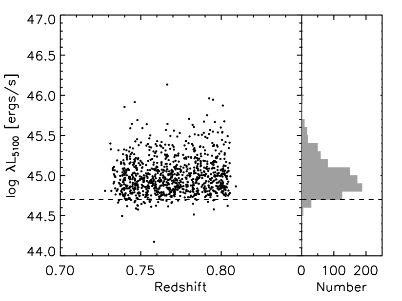
Since SDSS quasars are flux-limited in the survey, low luminosity quasars are lost in the SDSS sample. Figure 4 shows luminosity versus redshift for our sample. Because of the narrow redshift coverage for our sample, the minimum luminosity is almost constant and roughly estimated to be ergs/s.
3.2 Continuum and line fitting
In the UV to optical, the quasar continuum is composed of (i) the power-law continuum , (ii) the Balmer continuum and (iii) the Fe II pseudo-continuum . Thus we assumed a following formula as a model continuum :
| (6) |
3.2.1 Power-Law continuum
The power-law continuum is simply written as follows:
| (7) |
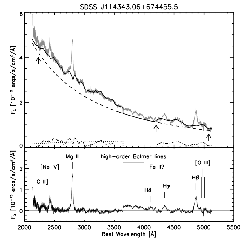
The free parameters of this model are a scaling factor and a power-law index . We chose three fitting ranges, 2200-2230 Å, 4180-4220 Å and 5050-5100 Å, as continuum windows, since these area have little emission lines (see Figure 5). There are, however, the Balmer continuum and the Fe II pseudo-continuum underneath these regions, requiring some corrections.
Tsuzuki et al. (2006) gives 14 quasar spectra covering a wide wavelength range and measured accurately their continuum levels. We fitted power-law continuum models to their spectra in the continuum windows, and compared the continuum levels with those given by Tsuzuki et al. (2006). We found that our method systematically overestimates the continuum levels, 10.1% at 2200-2230 Å, 5.7% at 4180-4220 Å and 3.4% at 5050-5100 Å. According to these results, we first reduced the flux densities of the object by these amount at each continuum window, then fitted the power-law continuum. An example of the fitted power-law continuum is indicated as the dashed line in Figure 5. The measurement error of the continuum levels is estimated to be less than 10%.
3.2.2 Balmer continuum
Grandi (1982) gives a formula describing the Balmer continuum produced by a uniform temperature, partially optically thick cloud:
| (8) |
where is the Planck function at the electron temperature , and is the optical depth at the Balmer edge at Å. Kurk et al. (2007) assumed gas clouds of uniform temperature ( K) and the optical depth fixed to , and fit equation (8) to their sample quasar spectra to estimate the strength of the Balmer continuum (see also Dietrich et al. 2003). We followed their method and assumed K, . The only one parameter, namely the scale factor , is set free and is decided by fitting equation (8) to the power-law subtracted spectrum at 36003645 Å. An example of the fitted Balmer continuum is indicated as the dotted line in Figure 5.
3.2.3 Fe II pseudo-continuum
Since Fe II has enormous energy levels, neighboring emission lines contaminate heavily with each other, which makes it difficult to measure the Fe II emission lines. One approach to measure the Fe II emission lines is to use Fe II templates. So far, several Fe II templates are derived from the narrow-line Seyfert 1 galaxy, I Zw 1.
In the UV, Vestergaard & Wilkes (2001) and Tsuzuki et al. (2006) give their Fe II templates. The template given by Vestergaard & Wilkes (2001) do not cover around Mg II line. Tsuzuki et al. (2006) used a synthetic spectrum calculated with the Cloudy photoionization code in order to separate the Fe II emission from the Mg II line, and derived semiempirically the Fe II template which covers around the Mg II line. Since we want to measure the Mg II emission line, we decided to use the UV Fe II template given by Tsuzuki et al. (2006).
In the optical, Véron-Cetty, Joly & Véron (2004) and Tsuzuki et al. (2006) open their Fe II templates to the public. Véron-Cetty et al. (2004) carefully analyzed the Fe II emission lines in I Zw 1, finding that the Fe II lines are emitted from both BLR and Narrow Line Region (NLR). They succeeded to separate them and called the broad line system L1 and the narrow line system N3, respectively. Tsuzuki et al. (2006) also analyzed the spectrum of I Zw 1 and derived the optical Fe II template, which was however not separated into the BLR and the NLR components. We applied both the broad line system L1 template given by Véron-Cetty et al. (2004) and the optical Fe II template given by Tsuzuki et al. (2006) to all of our samples, finding that the latter has a slightly smaller average value (median for Tsuzuki et al. 2006, while median for Véron-Cetty et al. 2004). Here we adopt to use the optical Fe II template given by Tsuzuki et al. (2006).
Prior to applying the Fe II template to each quasar, broadening of the template spectrum is needed. Thus we modeled the Fe II flux density as follows:
| (9) | |||||
where , is the velocity of light and represents the FWHM of the convolved Gauss function. We first calculated the equation (9) for km/s stepped by 100 km/s, thus prepared 51 Fe II emission line models. Then we flux-scaled each model to fit the continuum subtracted spectrum (i.e., the spectrum after subtracting the power-law and the Balmer continuum), and adopted the model which gives the smallest value. We decided mask regions as follows; 2280-2380Å for C II] 2326; 2400-2480Å for [Ne IV] 2423 and Fe III; 2750-2850Å for Mg II; 3647-4000Å for high-order Balmer lines; 4050-4150Å for H; 4300-4400Å for H; 4600-5050Å for He II 4686, H and [O III] 4959,5009. An example of the fitted Fe II pseudo-continuum is indicated as the dot-dashed line in Figure 5.
3.2.4 Mg II lines
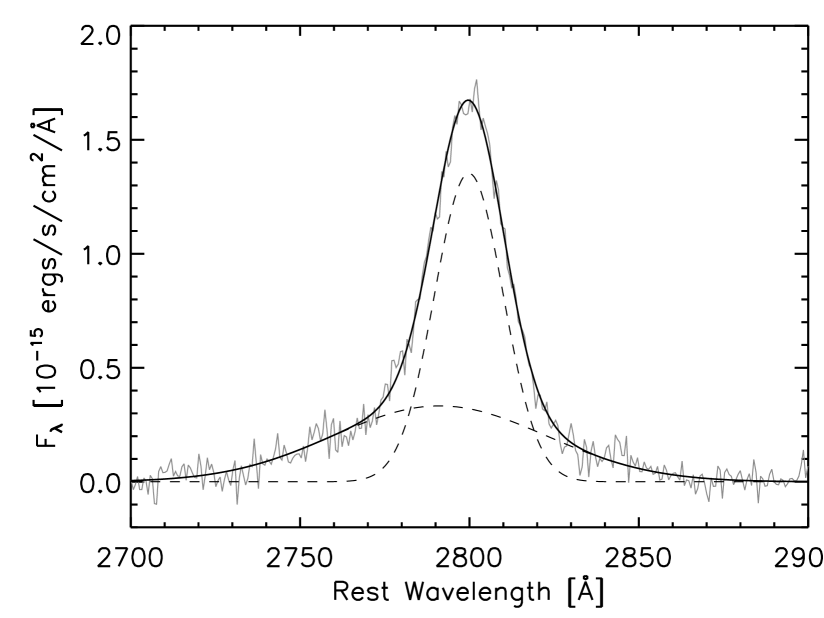
After subtracting the continuum components, we have measured the Mg II emission line for estimating the black hole mass from its FWHM. We have fitted the Mg II emission line profile by two gaussian components. Figure 6 shows an example of the Mg II emission line fitting.
3.3 Black hole mass and Eddington luminosity
For the classical black hole mass estimate in which the radiation pressure effect is neglected, we use the following formula given by McLure & Jarvis (2002):
| (10) |
The classical Eddington luminosity is given as follows:
| (11) |
where is the velocity of light, is the proton mass, and is the Thomson cross-section.
On the other hand, Marconi et al. (2008) suggested that the force of the radiation pressure should be corrected to derive the black hole mass. They give the radiation pressure corrected black hole mass and Eddington luminosity as follows:
| (12) |
| (13) |
| (14) |
where is the bolometric luminosity, is the total luminosity of the ionizing continuum (i.e., 13.6 eV), and is the ionizing photon fraction. The second term in the right hand side of equation (12) represents the correction term of the radiation pressure. We here adopt a bolometric correction given by Kaspi et al. (2000).
3.4 Error estimate
We performed a Monte-Carlo simulation similar to those done in Hu et al. (2008) for estimating the measurement errors. The detail of the procedure is as follows.
(i) Generating a composite spectrum. Following Vanden Berk et al. (2001), we generated a composite spectrum using all of our samples. This composite spectrum represents a typical quasar spectrum for our samples. (ii) Obtaining typical emission line profiles. We applied the measurement methods written in §3.2 to the composite spectrum, and obtained typical emission line profiles for Fe II(UV), Fe II(4570) and Mg II. (iii) Making artificial spectra. We combined these line profiles with the power-low continuum and the Balmer continuum. Thus the simulated spectrum is written as follows.
| (15) | |||||
Note that, for simplicity, we ignored the broadening of the pseudo-Fe II continuum. Values of input parameters, which are given in the parentheses in equation (15), are randomly sampled from probability distributions that are made to reflect the observations. Thus, we generated 1,000 simulated spectra. (iv) Generating a noise template. Using all the noise spectra produced by the SDSS pipeline for our samples, we generated a composite spectrum following Vanden Berk et al. (2001) and named it a noise template. This noise template is scaled so that the resulting median S/N to be 10 per pixel at the continuum level for each simulated spectrum, and is treated as its noise.
Now we have the 1,000 simulated spectra with their noise. The measurement methods written in §3.2 are applied to these simulated spectra. We calculate the value for each simulated spectrum where represents the input parameters (i.e., the values given in the parentheses in equation (15)) and represents the corresponding measured values for the simulated spectra. We regard , a standard deviation of , as error of the measurement. Thus we evaluate the measurement errors to be 16.4% for EW of Fe II(UV), 22.9% for EW of Fe II(4570) and 7.9% for FWHM(Mg II). The simulation implies the measurement error to be 2.9% for the luminosity, which is less than 10% estimated in the power-law fitting. Therefore we decided to evaluate the measurement error to be 10% for and .
4 Results and Discussion
4.1 On the excitation mechanism of Fe II emission
Figure 7 shows the observed Fe II(4570)/Fe II(UV) distribution. As can be seen from the comparison between this and Figure 2, our photoionization models underpredict the Fe II(4570)/Fe II(UV) by a factor of 10, failing to account for the observations. This result is consistent with the preceding study by Baldwin et al. (2004). Additional microturbulence to the photoionized clouds gets the situation even worse. Thus, Figure 7 seems to challenge classical photoionized pictures of Fe II-emitting clouds. On the other hand, in the case of the collisionally ionized models shown in Figure 3, the observed Fe II(4570)/Fe II(UV) flux ratios are well reproduced with and with K.
These results give two remarks: (1) the Fe II-emitting clouds in quasars are heated to K; (2) the UV and the X-ray photons, which are the heating source in our photoionization models, fail to heat the gas to such temperatures (probably heat the gas too hot!). One possible interpretation is that the Fe II-emitting clouds are heated by an alternative mechanism such as through shocks. Here we note that there is a reverberation mapping study implying shock heating for Fe II emission. Kuehn et al. (2008) analyzed optical Fe II emission bands in the Ark 120, finding that they do not respond to the continuum variation. Thus the optical Fe II-emitting region may be heated by other mechanism than photoionization. These results favor the shock heating for the optical Fe II-emitting region, but there are also difficulties. First, the amount of shock-processed matter would probably be too large. Second, as Kuehn et al. (2008) showed, collisionally ionized models failed to match the shape of the optical Fe II-emission band. Third, the fact that there is no response to the continuum variation for optical Fe II emission bands can also be interpreted as that the emitting region is too large to vary optical Fe II emission in observable timescales. Unless shocks are a viable solution, the failure of the photoionization model simply indicates that it is not predicting the correct heating rate, or that the radiative transport calculations are not correct.
One possible cause disturbing classical photoionization models to reproduce the observations may be the assumption that the Fe II emission is isotropic. Ferland et al. (2009) recently suggested that UV Fe II lines are beamed toward a central source while optical Fe II lines are emitted isotropically. Then photoionization models can reproduce the observed UV to optical Fe II flux ratio if the Fe II-emitting clouds are distributed asymmetrically so that we mainly observe their shielded faces. However, this needs special geometrical distributions like Type II AGNs; a thick Fe II-emitting gas surrounding the central source with a substantial covering factor, and intervening between the central region and our eyes. At the present time, it is not clear whether or not photoionization models can reproduce the emission line strengths other than Fe II under such the situation. Much broader exploration of photoionization model calculations is certainly needed.

4.2 Column density distribution inferred from Fe II(4570)/Fe II(UV)
Now we can roughly estimate column densities from the observed Fe II(4570)/Fe II(UV) by using equation (5). The estimated column density distribution is shown in Figure 8. An average and a standard deviation of the distribution are found to be . Marconi et al. (2009) has suggested that radiation pressure does play an important role in BLR gas dynamics if column densities of BLR clouds have intrinsic dispersion such as . Our results support that the assumption adopted in Marconi et al. (2009) is appropriate and that the radiation pressure plays an important role in BLR clouds.

4.3 Correlation between Eddington ratio and Fe II(4570)/Fe II(UV)
Figure 9 shows the relation between Fe II(4570)/Fe II(UV) and the Eddington ratio. A positive correlation is seen. Linear regression analysis, using an IDL procedure “FITEXY.pro” (cf. Press et al. 1992), gives the relation as:
| (16) |
The Spearman’s rank correlation coefficient333Spearman’s rank correlation coefficient is non-parametric measure of correlation, that is, which assesses how well an arbitrary monotonic function could describe the relationship between two variables without making any other assumptions for assessing the nonlinear correlation is . This means the probability of the null hypothesis that there is no correlation is less than . Thus the correlation between Fe II(4570)/Fe II(UV) and the Eddington ratio is real. This implies that the column density increases with the Eddington ratio, because Fe II(4570)/Fe II(UV) increases with the column density.
As was recently suggested by Dong et al. (2009), under the condition where the BLR clouds are subject to the radiation pressure, low-column-density clouds would be blown away by relatively large radiation pressure at large , so that only high-column-density clouds would be able to be gravitationally bound. Figure 9 is a supportive evidence for their suggestion.

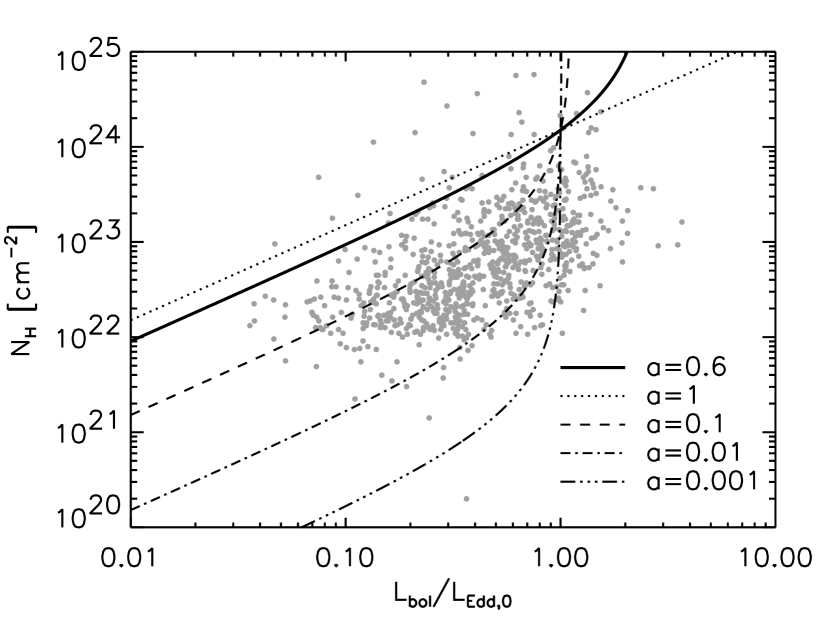
4.4 Super-Eddington problem
Figure 10 plots our samples on plane. Each line represents , so that the lower region of the line corresponds super-Eddington area. If we adopt ionizing photon fraction (i.e., thick solid line in Figure 10), which is an average value for AGNs calculated by Marconi et al. (2008), almost all of our samples become super-Eddington. This result can be interpreted in two ways: (i) the conversion from Fe II(4570)/Fe II(UV) to column densities (i.e, equation (5)) is wrong, or (ii) the adopted value of is inappropriate.
In the case (i), since Fe II(4570)/Fe II(UV) is a function of the column density and the temperature, the false in the conversion is attributed to the assumed temperature. If we assume hot clouds such as K, the corresponding column densities would become large, resulting in the solution for this super-Eddington problem. However, as already discussed, the previous studies favor cold clouds such as K for Fe II emission (cf. Collin et al. 1980, Joly 1987). Thus this interpretation seems to be inappropriate.
In the case (ii), as can be seen from Figure 10, if we adopt small values for such as 0.01, the majority of our samples becomes gravitationally bound. This means that the fraction of ionizing photons irradiating on Fe II-emitting clouds is much less than those on usual BLR clouds. Then it seems quite natural to conclude that the Fe II emission does not originate in the region where usual emission lines such as H originate, but originate in outer parts of BLR where the incident ionizing photon fraction becomes as low as . It is worth noting that from the studies of O I and Ca II emission lines, Matsuoka et al. (2008) also suggests that Fe II emission originates in outer parts of BLR.
4.5 Eigenvector 1 in terms of the column density
Boroson & Green (1992) applied a principal component analysis to low-redshift quasars and found that the principal component 1 (which is called “Eigenvector 1”) links the strength of optical Fe II emission and the weakness of [O III] emission. After a while, Boroson (2002) showed that Eigenvector 1 is driven predominantly by an Eddington ratio. However, the physical causes making up the Eigenvector 1 has been left unknown.
Here we propose a physical interpretation of Eigenvector 1 in terms of the column density. As discussed in the previous section, small-column-density clouds would be driven away from the line-emitting region by the radiation pressure at large Eddington ratio, and only large-column-density clouds can be gravitationally bound. Radiative transfer effects make the optical Fe II emission become large in such large-column-density clouds. On the other hand, ionizing photons emitted from the central object are intervened by these large-column-density clouds and thus have less probabilities of ionizing photons reaching to NLR clouds, resulting in weak [O III] emission. In fact, Figure 10(t) in Tsuzuki et al. (2006) shows a negative correlation between the [O III]/H and Fe II(O1)/Fe II(U1), which is almost the same as our Fe II(4570)/Fe II(UV), for 14 quasars.
5 Summary
-
1.
Analysis of the Fe II(UV), Fe II(4570) and Mg II emission lines is performed for 884 SDSS quasars in a redshift range of .
-
2.
We suggest that Fe II(4570)/Fe II(UV) can be an indicator of the column density of Fe II-emitting clouds regardless of the excitation mechanism, i.e., photoionized or collisionally ionized clouds. From model calculations, we have confirmed this suggestion.
-
3.
Our photoionization models underpredict Fe II(4570)/Fe II(UV) by a factor of 10, consistent with the preceding studies. Unless shocks are a viable heating mechanism, the failure of the photoionization model simply indicates that it is not predicting the correct heating rate, or that the radiative transport calculations are not correct. Ignoring anisotropy of UV Fe II emission may be one of the causes.
-
4.
The column density distribution estimated from Fe II(4570)/Fe II(UV) is almost the same as the one suggested by Marconi et al. (2009), supporting that the radiation pressure does work on Fe II-emitting clouds.
-
5.
We also find a positive correlation between Fe II(4570)/Fe II(UV) and the Eddington ratio, implying the links between the column density and the Eddington ratio.
-
6.
We find that under the assumption of the ionization fraction , almost all of our samples become super-Eddington. This problem can be cleared if the Fe II emission originates in outer parts of BLR where the ionizing photon fraction becomes as low as .
-
7.
We propose physical interpretation of ’Eigenvector 1’ in terms of the column density. In the interpretation, the strength of the optical Fe II emission results in the radiative transfer effects, while the weakness of the [O III] emission results in the reduction of ionizing photons in NLR caused by intervening large column density BLR clouds.
Acknowledgments
We thank the anonymous referee for providing us with very helpful comments. This work was supported in part by Grant-in-Aid for JSPS Fellows, Scientific research (20001003), Specially Promoted Research on Innovative Areas (22111503), Research Activity Start-up (21840027), and Young Scientists (22684005).
References
- Baldwin et al. (2004) Baldwin J.A., Ferland G.J., Korista K.T., Hamann F., LaCluyzé A., 2004, ApJ, 615, 610
- Baldwin et al. (1995) Baldwin J., Ferland G., Korista K., Verner D., 1995, ApJ, 455, L119
- Boroson (2002) Boroson T.A., 2002, ApJ, 565, 78
- Boroson & Green (1992) Boroson T.A., Green R.F., 1992, ApJS, 80, 109
- Collin & Joly (2000) Collin S., Joly M., 2000, New Astron. Rev., 44, 531
- Collin et al. (1980) Collin-Souffrin S., Joly M., Dumont S., Heidmann N., 1980, A&A, 83, 190
- Dietrich et al. (2002) Dietrich M., Appenzeller I., Vestergaard M., Wagner S.J., 2002, ApJ, 564, 581
- Dietrich et al. (2003) Dietrich M., Hamann F., Appenzeller I., Vestergaard M., 2003, ApJ, 596, 817
- Dong et al. (2009) Dong X., Wang J., Wang T., Wang H., Fan X., Zhou H., Yuan W., 2009a, arXiv, 0903, 5020
- Elston et al. (1994) Elston R., Thompson K.L., Hill G.J., 1994, Nat., 367, 250
- Ferland et al. (2009) Ferland G.J., Hu C., Wang J.M., Baldwin J.A., Porter R.L., van Hoof P.A.M., Williams R.J.R., 2009, arXiv, 0911, 1173
- Ferland et al. (1998) Ferland G.J., Korista K.T., Verner D.A., Ferguson J.W., Kingdon J.B., Verner E.M., 1998, PASP, 110, 761
- Freudling et al. (2003) Freudling W., Corbin M.R., Korista K.T., 2003, ApJ, 587, L67
- Grandi (1982) Grandi S.A., 1982, ApJ, 255, 25
- Hamann & Ferland (1993) Hamann F., Ferland G., 1993, ApJ, 418, 11
- Hu et al. (2008) Hu C., Wang J.M., Ho L.C., Chen Y.M., Zhang H.T., Bian W.H., Xue S.J., 2008, ApJ, 687, 78
- Iwamuro et al. (2002) Iwamuro F., Motohara K., Maihara T., Kimura M., Yoshii Y., Doi M., 2002, ApJ, 565, 631
- Iwamuro et al. (2004) Iwamuro F., Kimura M., Eto S., Maihara T., Motohara K., Yoshii Y., Doi M., 2004, ApJ, 614, 691
- Joly (1987) Joly M., 1987, A&A, 184, 33
- Kaspi et al. (2000) Kaspi S., Smith P.S., Netzer H., Maoz D., Jannuzi B.T., Giveon U., 2000, ApJ, 533, 631
- Kawara et al. (1996) Kawara K., Murayama T., Taniguchi Y., Arimoto N., 1996, ApJ, 470, 85
- Kuehn et al. (2008) Kuehn C.A., Baldwin J.A., Peterson B.M., Korista K.T., 2008, ApJ, 673, 69
- Kurk et al. (2007) Kurk J.D. et al., 2007, ApJ, 669, 32
- Maiolino et al. (2003) Maiolino R., Juarez Y., Mujica R., Nagar N.M., Oliva E., 2003, ApJ, 596, L155
- Maoz et al. (1993) Maoz D. et al., 1993, ApJ, 404, 576
- Marconi et al. (2009) Marconi A. et al., 2009, ApJ, 698, 103
- Marconi et al. (2008) Marconi A. et al., 2008, ApJ, 678, 693
- Matsuoka et al. (2008) Matsuoka Y., Kawara K., Oyabu S., 2008, ApJ, 673, 62
- Matsuoka et al. (2007) Matsuoka Y., Oyabu S., Tsuzuki Y., Kawara K., 2007, ApJ, 663, 781
- Matteucci et al. (2006) Matteucci F., Panagia N., Pipino A., Mannucci F., Recchi S., Della Valle M., 2006, MNRAS, 372, 265
- McLure & Jarvis (2002) McLure R.J., Jarvis M.J., 2002, MNRAS, 337, 109
- Nagao et al. (2001) Nagao T., Murayama T., Taniguchi Y., 2001, ApJ, 546, 744
- Netzer (2009) Netzer H., 2009, ApJ, 695, 793
- Netzer & Wills (1983) Netzer H., Wills B.J., 1983, ApJ, 275, 445
- Pei (1992) Pei Y.C., 1992, ApJ, 395, 130
- Phillips (1978) Philips M.M., 1978, ApJ, 226, 736
- Press et al. (1992) Press W.H., Teukolsky S.A., Vetterling W.T., Flannery B.P., 1992, Numerical Recipes. Cambridge Univ. Press, Cambridge
- Sameshima et al. (2009) Sameshima H. et al., 2009, MNRAS, 395, 1087
- Schlegel et al. (1998) Schlegel D.J., Finkbeiner D.P., Davis M., 1998, ApJ, 500, 525
- Schneider et al. (2007) Schneider D.P. et al., 2007, AJ, 134, 102
- Totani et al. (2008) Totani T., Morokuma T., Oda T., Doi M., Yasuda N., 2008, PASJ, 60, 1327
- Tsuzuki et al. (2006) Tsuzuki Y., Kawara K., Yoshii Y., Oyabu S., Tanabé T., Matsuoka Y., 2006, ApJ, 650, 57
- Vanden Berk et al. (2001) Vanden Berk D.E. et al., 2001, AJ, 122, 549
- Verner et al. (2003) Verner E., Bruhweiler F., Verner D., Johansson S., Gull T., 2003, ApJ, 592, L59
- Verner et al. (1999) Verner E.M., Verner D.A., Korista K.T., Ferguson J.W., Hamann F., Ferland G.J., 1999, ApJS, 120, 101
- Véron-Cetty et al. (2004) Véron-Cetty M.P., Joly M., Véron P., 2004, A&A, 417, 515
- Vestergaard & Wilkes (2001) Vestergaard M., Wilkes B.J., 2001, ApJS, 134, 1
- Yoshii et al. (1996) Yoshii Y., Tsujimoto T., Nomoto K., 1996, ApJ, 462, 266
- Yoshii et al. (1998) Yoshii Y., Tsujimoto T., Kawara K., 1998, ApJ, 507, 113