Implicit Neural Representations and the
Algebra of Complex Wavelets
Abstract
Implicit neural representations (INRs) have arisen as useful methods for representing signals on Euclidean domains. By parameterizing an image as a multilayer perceptron (MLP) on Euclidean space, INRs effectively represent signals in a way that couples spatial and spectral features of the signal that is not obvious in the usual discrete representation, paving the way for continuous signal processing and machine learning approaches that were not previously possible. Although INRs using sinusoidal activation functions have been studied in terms of Fourier theory, recent works have shown the advantage of using wavelets instead of sinusoids as activation functions, due to their ability to simultaneously localize in both frequency and space. In this work, we approach such INRs and demonstrate how they resolve high-frequency features of signals from coarse approximations done in the first layer of the MLP. This leads to multiple prescriptions for the design of INR architectures, including the use of complex wavelets, decoupling of low and band-pass approximations, and initialization schemes based on the singularities of the desired signal.
1 Introduction
Implicit neural representations (INRs) have emerged as a set of neural architectures for representing and processing signals on low-dimensional spaces. By learning a continuous interpolant of a set of sampled points, INRs have enabled and advanced state-of-the-art methods in signal processing (Xu et al., 2022) and computer vision (Mildenhall et al., 2020).
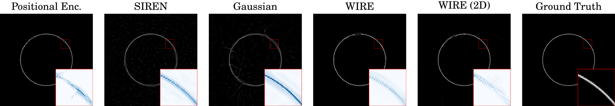
Typical INRs are specially designed multilayer perceptrons (MLPs), where the activation functions are chosen in such a way to yield a desirable signal representation; some of these methods are demonstrated on a simple test image in Fig. 1.
Although these INRs can be easily understood at the first layer due to the simplicity of plotting the function associated to each neuron based on its weights and biases, the behavior of the network in the second layer and beyond is more opaque, apart from some theoretical developments in the particular case of a sinusoidal first layer (Yüce et al., 2022).
This work develops a broader theoretical understanding of INR architectures with a wider class of activation functions, followed by practical prescriptions rooted in time-frequency analysis. In particular, we
-
1.
Characterize the function class of INRs in terms of Fourier convolutions of the neurons in the first layer (Theorem 1)
-
2.
Demonstrate how INRs that use complex wavelet functions preserve useful properties of the wavelet, even after the application of the nonlinearities (Corollary 4)
-
3.
Suggest a split architecture for approximating signals, decoupling the smooth and nonsmooth parts into linear and nonlinear INRs, respectively (Section 4.3)
-
4.
Leverage connections with wavelet theory to propose efficient initialization schemes for wavelet INRs based on the wavelet modulus maxima for capturing singularities in the target functions (Section 5).
Following a brief survey of INR methods, the class of architectures we study is defined in Section 2. The main result bounding the function class represented by these architectures is stated in Section 3, which is then related to the algebra of complex wavelets in Section 4. The use of the wavelet modulus maxima for initialization of wavelet INRs is described and demonstrated in Section 5, before concluding in Section 6.
2 Implicit Neural Representations
Wavelets as activation functions in MLPs have been shown to yield good function approximators (Zhang & Benveniste, 1992; Marar et al., 1996). These works have leveraged the sparse representation of functions by wavelet dictionaries in order to construct simple neural architectures and training algorithms for effective signal representation. Indeed, an approximation of a signal by a finite linear combination of ridgelets (Candès, 1998) can be viewed as one such MLP using wavelet activation functions.
Recently, sinusoidal activation functions in the first layer (Tancik et al., 2020) and beyond (Sitzmann et al., 2020; Fathony et al., 2020) have been shown to yield good function approximators, coupled with a harmonic analysis-type bound on the function class represented by these networks (Yüce et al., 2022). Other methods have used activation functions that, unlike sinusoids, are localized in space, such as gaussians (Ramasinghe & Lucey, 2021) or Gabor wavelets (Saragadam et al., 2023).
Following the formulation of (Yüce et al., 2022), we define an INR to be a map defined in terms of a function , followed by an MLP with analytic111That is, entire on . activation functions for layers :
| (1) | ||||
where denotes the set of parameters dictating the tensor , matrices and , and vectors for , with fixed integers satisfying . We will henceforth refer to as the template function of the INR. Owing to the use of Gabor wavelets by Saragadam et al. (2023), we will refer to functions of the form (1) as WIRE INRs, although (1) also captures architectures that do not use wavelets, such as SIREN (Sitzmann et al., 2020).
3 Main Results
For the application of INRs to practical problems, it is important to understand the function class that an INR architecture can represent. We will demonstrate how the function parameterized by an INR can be understood via time-frequency analysis, ultimately motivating the use of wavelets as template functions.
3.1 Expressivity of INRs
Noting that polynomials of sinusoids generate linear combinations of integer harmonics of said sinusoids, Yüce et al. (2022) bounded the expressivity of SIREN (Sitzmann et al., 2020) and related architectures (Fathony et al., 2020). These results essentially followed from identities relating products of trigonometric functions. For template functions that are not sinusoids, such as wavelets (Saragadam et al., 2023), these identities do not hold. The following result offers a bound on the class of functions represented by an INR.
Theorem 1.
Let be a WIRE INR. Assume that each of the activation functions is a polynomial of degree at most , and that the Fourier transform of the template function exists.222It may exist only in the sense of tempered distributions. Let for each having full rank, and also let for . For , denote by the set of ordered -tuples of nonnegative integers such that .
Let a point be given. Then, there exists an open neighborhood such that for all
| (2) |
for coefficients independent of , where denotes -fold convolution333-fold convolution is defined by convention to yield the Dirac delta. of the argument with itself with respect to . Furthermore, the coefficients are only nonzero when each such that also satisfies .
The proof is left to Appendix A. Theorem 1 illustrates two things. First, the output of an INR has a Fourier transform determined by convolutions of the Fourier transforms of the atoms in the first layer with themselves, serving to generate “integer harmonics” of the initial atoms determined by scaled, shifted copies of the template function . Notably, this recovers (Yüce et al., 2022, Theorem 1). Second, the support of these scaled and shifted atoms is preserved, so that the output at a given coordinate is dependent only upon the atoms in the first layer whose support contains .
Remark 2.
The assumptions behind Theorem 1 can be relaxed to capture a broader class of architectures. By imposing continuity conditions on the template function , the activation functions can be reasonably extended to analytic functions. These extensions are discussed in Appendix B.
3.2 Effective Time-Frequency Support of INRs
As noted before, Theorem 1 describes the output of an INR at a point by self-convolutions of sums of the Fourier transforms of the atoms in the first layer whose support contains that point. So, for the remainder of this section, we can assume that is fixed, and that we only consider indices such that .
Assume that the template function has compact support, which precludes from having compact support. However, if we make the further assumption that is smooth, then is rapidly decreasing. We will then say, informally, that has a compact effective support, denoted by the set . Making the approximation , we have that .
As a first approximation, then, we can estimate the frequency support “locally” around the point , in the sense of the Fourier transform following multiplication with a suitable cutoff function. Examining the summands in (2), the support of the self-convolutions in the Fourier domain are bounded by
where the subset relationship is understood to be in the informal sense of effective support, and the sum on the RHS is understood as the Minkowski sum of the summands . So, the frequency support described by Theorem 1 is effectively bounded by the set
4 The Algebra of Complex Wavelets
Of the INR architectures surveyed in Section 2, the only one to use a complex wavelet template function is WIRE (Saragadam et al., 2023), where a Gabor wavelet is used. Gabor wavelets are essentially asymmetric (in the Fourier domain) band-pass filters, which are necessarily complex-valued due to the lack of conjugate symmetry in the Fourier domain. We now consider the advantages of using complex wavelets, or more precisely progressive wavelets, as template functions for INRs by examining their structure as an algebra of functions.
4.1 Progressive Template Functions
For the sake of discussion, suppose that , so that the INR represents a 1D function. The template function is said to be progressive444More commonly known as an analytic signal, we use this terminology to avoid confusion with the analytic activation functions used in the INR. if it has no negative frequency components, i.e., for , we have (Mallat, 1999). If is integrable, its Fourier transform is uniformly continuous, which implies that for integrable progressive functions we have . Without embarking upon a long review of progressive wavelets (Mallat, 1999), we discuss some of the basic properties of progressive functions that are relevant to the discussion at hand. It is obvious that progressive functions remain progressive under scalar multiplication, shifts, and positive scaling. That is, for arbitrary , if is progressive, then the function is also progressive. Moreover, progressive functions are closed under multiplication, so that if and are progressive, then is also progressive,555This is a simple consequence of the convolution theorem. i.e., progressive functions constitute an algebra over .
Example 1 (Complex Sinusoid).
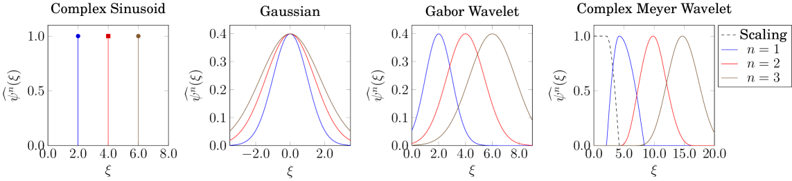
For any , the complex sinusoid is a progressive function, as its Fourier transform is a Dirac delta centered at . As pictured in Fig. 2 (Left), the exponents are themselves complex sinusoids, where .
Example 2 (Gaussian).
The gaussian function, defined for some as , is not a progressive function, as its Fourier transform is symmetric and centered about zero. Moreover, as pictured in Fig. 2 (Center-Left), the exponents are also gaussian functions , which also have Fourier transform centered at zero. Unlike the complex sinusoid, the powers of the gaussian are all low-pass, but with increasingly wide passband.
Example 3 (Gabor Wavelet).
For any , the Gabor wavelet defined as is not a progressive function, as its Fourier transform is a gaussian centered at with standard deviation . However, the Fourier transform of the exponents for integers are gaussians centered at with standard deviation , as pictured in Fig. 2 (Center-Right). So, as grows sufficiently large, the effective support of will be contained in the positive reals, so that the Gabor wavelet can be considered as a progressive function for the purposes of studying INRs.
A progressive function on has Fourier support contained in the nonnegative real numbers. Of course, there is not an obvious notion of nonnegativity that generalizes to for . Noting that the nonnegative reals form a convex conic subset of , we define the notion of a progressive function with respect to some conic subset of :
Definition 3.
Let be a convex conic set, i.e., for all and , we have that .666We henceforth refer to such sets as simply “conic.” A function is said to be -progressive if . The function is said to be locally -progressive at if there exists some -progressive function so that for all smooth functions with support in a sufficiently small neighborhood of , we have
| (3) |
Curvelets (Candès & Donoho, 2004), for instance, are typically defined in a way to make them -progressive for some conic set that indicates the oscillatory direction of a curvelet atom. Observe that if is a conic set, then for any matrix , the set is also conic. Thus, for a function that is -progressive, the function is -progressive.
Observe further that for two -progressive functions , their product is also -progressive. The closure of progressive functions under multiplication implies that an analytic function applied pointwise to a progressive function is progressive. For INRs as defined in (1), this yields the following corollary to Theorem 1.
Corollary 4.
Let be conic, and let be given, with Fourier support denoted . Let for each having full rank. Assume that for each , we have . Then, the WIRE INR defined by (1) is a -progressive function.
Moreover, if we fix some , and if the assumption holds for the indices such that , then is locally -progressive at .
The proof is left to Appendix C. Corollary 4 shows that INRs preserve the Fourier support of the transformed template functions in the first layer up to conic combinations, so that any advantages/limitations of approximating functions using such -progressive functions are maintained.
Remark 5.
One may notice that a -progressive function will always incur a large error when approximating a real-valued function, as real-valued functions have conjugate symmetric Fourier transforms (apart from the case ). For fitting real-valued functions, it is effective to simply fit the real part of the INR output to the function, as taking the real part of a function is equivalent to taking half of the sum of that function and its conjugate mirror in the Fourier domain. In the particular case of , fitting the real part of a progressive INR to a function is equivalent to fitting the INR to that function’s Hilbert transform.
4.2 Band-pass Progressive Wavelets
Corollary 4 holds for conic sets , but is also true for a larger class of sets. If some set is conic, it is by definition closed under all sums with nonnegative coefficients. Alternatively, consider the following weaker property:
Definition 6.
Let . is said to be weakly conic if for all and , we have that , and that . A function is said to be -progressive if . The function is said to be locally -progressive at if there exists some -progressive function so that for all smooth functions with support in a sufficiently small777Again, not necessarily compact. neighborhood of , we have
| (4) |
The notion of a weakly conic set is illustrated in Fig. 3 (Left). Just as in the case of progressive functions for a conic set, the set of -progressive functions for a weakly conic set constitutes an algebra over . One can check, then, that Corollary 4 holds for weakly conic sets as well. Putting this into context, consider a template function such that vanishes in some neighborhood of the origin. Assume furthermore that is contained in some weakly conic set .
Example 4 (Complex Meyer Wavelet).
The complex Meyer wavelet is most easily defined in terms of its Fourier transform. Define
The complex Meyer wavelet and its exponents are pictured in Fig. 2 (Right). Observe that these functions are not only progressive, but are also -progressive for the weakly conic set . The Meyer scaling function, pictured by the dashed line in Fig. 2 (Right), has Fourier support that only overlaps that of the complex Meyer wavelet, but none of its powers.
Applying this extension of Corollary 4, we see that if the atoms in the first layer of an INR using such a function have vanishing Fourier transform in some neighborhood of the origin, then the output of the INR has Fourier support that also vanishes in that neighborhood.
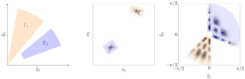
We illustrate this in using a template function where is the tensor product of a gaussian and a complex Meyer wavelet. Using this template function, we construct an INR with in the first layer, and a single polynomial activation function. The modulus of the sum of the template functions before applying the activation function is shown in Fig. 3 (Center). We then plot the modulus of the Fourier transform of in Fig. 3 (Right). First, observe that since the effective supports of the transformed template functions are supported by two disjoint sets, the Fourier transform of can be separated into two cones, each corresponding to a region in . Second, since the complex Meyer wavelet vanishes in a neighborhood of the origin, these cones are weakly conic, so that the Fourier transform of vanishes in a neighborhood of the origin as well, by Corollary 4 applied to weakly conic sets.
Remark 7.
The weakly conic sets pictured in Fig. 3 (Right) are only approximation bounds of the true Fourier support of the constituent atoms. We see that Corollary 4 still holds in an approximate sense, as the bulk of the Fourier support of the atoms is contained in each of the pictured cones.
4.3 A Split Architecture for INRs
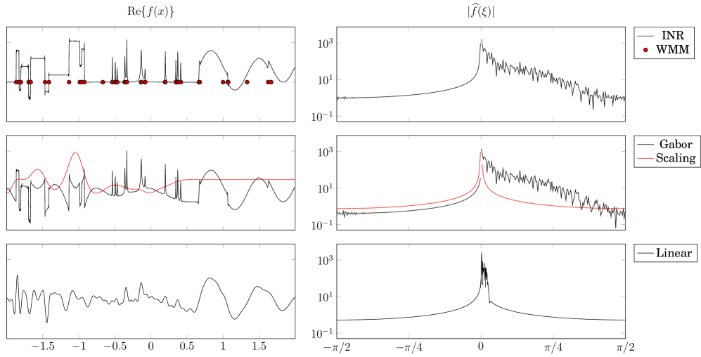
Based on this property of INRs preserving the band-pass properties of progressive template functions, it is well-motivated to approximate functions using a sum of two INRs: one to handle the low-pass components using a scaling function, and the other to handle the high-pass components using a wavelet. We illustrate this in Fig. 4, where we fit two INRs to a test signal on (Donoho & Johnstone, 1994).
The first INR uses a gaussian template function with , and the constraint that the weights are all equal to one, i.e., the template atoms only vary in their abscissa. Such a network is essentially a single-layer perceptron (Zhang & Benveniste, 1992) for representing smooth signals. We refer to this network as the “scaling INR.”
The second INR uses a Gabor template function with , where we initialize the weights in the first layer to be positive, thus satisfying the condition of in Corollary 4 for . Although is not progressive, its Fourier transform has fast decay, so we consider it to be essentially progressive, and thus approximately fulfilling the conditions of Corollary 4. We refer to this network as the “Gabor INR,” as it is the WIRE architecture (Saragadam et al., 2023) for signals on .
The reason for modeling a signal as the sum of a linear scaling INR and a nonlinear INR with a Gabor wavelet is apparent in Fig. 2 (Right), where the scaling function and powers of a complex Meyer wavelet are pictured. Observe that the portions of the Fourier spectrum covered by the scaling function and the high powers of the Gabor wavelet (as in an INR, by Theorem 1) are essentially disjoint. The idea behind this architecture is to use a simple network to approximate the smooth parts of the target signal, and then a more complicated nonlinear network to approximate the nonsmooth parts of the signal.
We plot the real part of the sum of the scaling INR and Gabor INR in Fig. 4 (Top) along with the individual network outputs in Fig. 4 (Center). One can clearly see how the scaling INR captures the low-pass components of the signal, while the Gabor INR captures the transient behavior.
To see the role of the nonlinearities in the Gabor INR, we freeze the weights and biases in the first layer of the Gabor INR, and take an optimal linear combination of the resulting template atoms to fit the signal, thus yielding an INR with no nonlinearities beyond the template functions (Zhang & Benveniste, 1992). The real part of the resulting function is plotted in Fig. 4 (Bottom), where the singularities from the Gabor INR are severely smoothed. This reflects how the activation functions resolve high-frequency features from low-frequency approximations, as illustrated initially in Fig. 3.
5 Resolution of Singularities
A useful model for studying sparse representations of images is the cartoon-like image, which is a smooth function on apart from singularities along a twice-differentiable curve (Candès & Donoho, 2004; Wakin et al., 2006).
The smooth part of an image can be handled by the scaling function associated to a wavelet transform, while the singular parts are best captured by the wavelet function. In the context of the proposed split INR architecture, the scaling INR yields a smooth approximation to the signal, and the Gabor INR resolves the remaining singularities.
5.1 Initialization With the Wavelet Modulus Maxima
As demonstrated by Theorem 1, the function in the first layer of an INR determines the expressivity of the network. Many such networks satisfy a universal approximation property (Zhang & Benveniste, 1992), but their value in practice comes from their implicit bias (Yüce et al., 2022; Saragadam et al., 2023) in representing a particular class of functions. For instance, using a wavelet in the first layer results in sharp resolution of edges with spatially compact error (Saragadam et al., 2023). In the remainder of this section, we demonstrate how an understanding of singular points in terms of the wavelet transform can be used to bolster INR architectures and initialization schemes.
Roughly speaking, isolated singularities in a signal are points where the signal is nonsmooth, but is smooth in a punctured neighborhood around that point. Such singularities generate “wavelet modulus maxima” (WMM) curves in the continuous wavelet transform (Mallat, 1999), which have slow decay in the Fourier domain. With Theorem 1 in mind, we see that INRs can use a collection of low-frequency template atoms and generate a collection of coupled high-frequency atoms, while also preserving the spatial locality of the template atoms.
The combination of these insights suggests a method for the initialization of INRs. In particular, for a given number of template atoms in an INR, the network weights and abscissa should be initialized in a way that facilitates effective training of the INR via optimization methods.
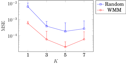
We empirically demonstrate the difference in performance for INRs initialized at random and INRs initialized in accordance with the singularities in the target signal. Once again, we fit the sum of a scaling INR and a Gabor INR to the target signal in Fig. 4. In Fig. 5, we plot the mean squared error (MSE) for this setting after training steps for both randomly initialized and strategically initialized INRs, for , where and is the number of WMM points as determined by an estimate of the continuous wavelet transform of the target signal. The randomly initialized INRs have abscissa distributed uniformly at random over the domain of the signal. The strategically initialized INRs place template atoms at each WMM point (so, a deterministic set of abscissa points). Both initialization schemes randomly distribute the scale weights uniformly in the interval . We observe that for all , the MSE of the strategically initialized INR is approximately an order of magnitude less than that of the randomly initialized INR.
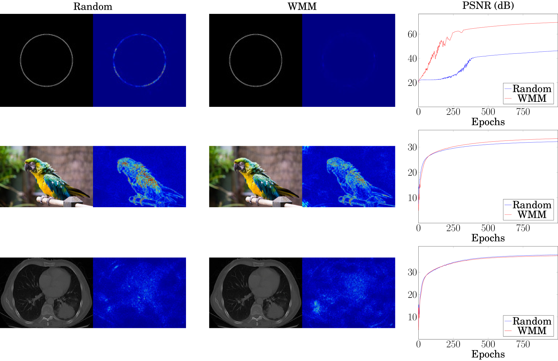
When , e.g., images, the WMM can be approximated by the gradients of the target signal to obtain an initial set of weights and biases for the Gabor INR. We evaluate this empirically on a set of images shown in Fig. 6. For each example, we approximate the target image using the proposed split INR architecture. For the WMM-based initialization, we apply a Canny edge detector (Canny, 1986) to encode the positions and directions of the edges. Further details can be found in Appendix D. We then used a subset of edge locations for biases of the first layer of the Gabor INR. For simplicty, we initialized the weights such that each neuron generates a radially symmetric Gabor filter. For images consisting of isolated singularities, such as the circular edge example in the first row in Fig. 6, we observe that a WMM-based initialization results in nearly dB higher PSNR, along with faster convergence rates than its uninitialized counterpart. A similar but less significant advantage can be seen for other images, such as the parrot with a blurred background (second row in Fig. 6). WMM-based initialization, has limited advantages when the image has dense texture, such as the chest X-ray scan (third row in Fig. 6). Overall, we observe that WMM-based initialization has similar advantages for signals on both and .
6 Conclusions
We have offered a time-frequency analysis of INRs, leveraging polynomial approximations of the behavior of MLPs beyond the first layer. By noting that progressive functions form an algebra over the complex numbers, we demonstrated that this analysis yields insights into the behavior of INRs using complex wavelets, such as WIRE (Saragadam et al., 2023). This naturally leads to a split architecture for approximating signals, which decouples the low-pass and high-pass parts of a signal using two INRs, roughly corresponding to the scaling and wavelet functions of a wavelet transform. Furthermore, the connection with the theory of wavelets yields a natural initialization scheme for the weights of an INR based on the wavelet modulus maxima of a signal.
INR architectures built using wavelet activation functions offer useful advantages for function approximation that balance locality in space and frequency. The structure of complex wavelets as an algebra of functions with conic Fourier support, combined with the application of INRs for interpolating sampled functions, suggests a connection with microlocal and semiclassical analysis (Monard & Stefanov, 2023). As future work, we aim to extend the results of this paper to synthesize true singularities at arbitrarily fine scales, despite the continuous and non-singular structure of INR approximations of a sampled signal. We also foresee the decoupling of the smooth and singular parts of a signal by the split INR architecture having useful properties for solving inverse problems and partial differential equations.
Acknowledgements
This work was supported by NSF grants CCF-1911094, IIS-1838177, and IIS-1730574; ONR grants N00014-18-1-2571, N00014-20-1-2534, and MURI N00014-20-1-2787; AFOSR grant FA9550-22-1-0060; and a Vannevar Bush Faculty Fellowship, ONR grant N00014-18-1-2047. Maarten de Hoop gratefully acknowledges support from the Department of Energy under grant DE-SC0020345, the Simons Foundation under the MATH+X program, and the corporate members of the Geo-Mathematical Imaging Group at Rice University.
References
- Candès (1998) Emmanuel Jean Candès. Ridgelets: theory and applications. PhD thesis, Stanford University, 1998.
- Candès & Donoho (2004) Emmanuel Jean Candès and David Leigh Donoho. New tight frames of curvelets and optimal representations of objects with piecewise singularities. Communications on Pure and Applied Mathematics, 57(2):219–266, 2004.
- Canny (1986) John Canny. A computational approach to edge detection. IEEE Transactions on Pattern Analysis and Machine Intelligence, (6):679–698, 1986.
- Donoho & Johnstone (1994) David Leigh Donoho and Iain M Johnstone. Ideal spatial adaptation by wavelet shrinkage. Biometrika, 81(3):425–455, 1994.
- Fathony et al. (2020) Rizal Fathony, Anit Kumar Sahu, Devin Willmott, and J Zico Kolter. Multiplicative filter networks. In International Conference on Learning Representations, 2020.
- Mallat (1999) Stéphane Mallat. A wavelet tour of signal processing. Elsevier, 1999.
- Marar et al. (1996) Joao Fernando Marar, Edson CB Carvalho Filho, and Germano C Vasconcelos. Function approximation by polynomial wavelets generated from powers of sigmoids. In Wavelet Applications III, volume 2762, pp. 365–374. SPIE, 1996.
- Mildenhall et al. (2020) Ben Mildenhall, Pratul P Srinivasan, Matthew Tancik, Jonathan T Barron, Ravi Ramamoorthi, and Ren Ng. NeRF: Representing scenes as neural radiance fields for view synthesis. In IEEE European Conference on Computer Vision, 2020.
- Monard & Stefanov (2023) François Monard and Plamen Stefanov. Sampling the X-ray transform on simple surfaces. SIAM Journal on Mathematical Analysis, 55(3):1707–1736, 2023.
- Ramasinghe & Lucey (2021) Sameera Ramasinghe and Simon Lucey. Beyond periodicity: Towards a unifying framework for activations in coordinate-MLPs. In IEEE European Conference on Computer Vision, 2021.
- Saragadam et al. (2023) Vishwanath Saragadam, Daniel LeJeune, Jasper Tan, Guha Balakrishnan, Ashok Veeraraghavan, and Richard G Baraniuk. WIRE: Wavelet implicit neural representations. In IEEE/CVF Computer Vision and Pattern Recognition Conference, pp. 18507–18516, 2023.
- Sitzmann et al. (2020) Vincent Sitzmann, Julien Martel, Alexander Bergman, David Lindell, and Gordon Wetzstein. Implicit neural representations with periodic activation functions. Advances in Neural Information Processing Systems, 2020.
- Tancik et al. (2020) Matthew Tancik, Pratul P. Srinivasan, Ben Mildenhall, Sara Fridovich-Keil, Nithin Raghavan, Utkarsh Singhal, Ravi Ramamoorthi, Jonathan T. Barron, and Ren Ng. Fourier features let networks learn high frequency functions in low dimensional domains. Advances in Neural Information Processing Systems, 2020.
- Wakin et al. (2006) Michael B Wakin, Justin K Romberg, Hyeokho Choi, and Richard G Baraniuk. Wavelet-domain approximation and compression of piecewise smooth images. IEEE Transactions on Signal Processing, 15(5):1071–1087, 2006.
- Xu et al. (2022) Dejia Xu, Peihao Wang, Yifan Jiang, Zhiwen Fan, and Zhangyang Wang. Signal processing for implicit neural representations. Advances in Neural Information Processing Systems, 35, 2022.
- Yüce et al. (2022) Gizem Yüce, Guillermo Ortiz-Jiménez, Beril Besbinar, and Pascal Frossard. A structured dictionary perspective on implicit neural representations. In IEEE/CVF Computer Vision and Pattern Recognition Conference, 2022.
- Zhang & Benveniste (1992) Qinghua Zhang and Albert Benveniste. Wavelet networks. IEEE Transactions on Neural Networks, 3(6):889–898, 1992.
Appendix A Proof of Theorem 1
Let be given, and let be the set of indices such that . Then, there exists an open neighborhood such that for all , for any . Thus, for any , the assumptions on the activation functions imply that is expressible as a complex multivariate polynomial of with degree at most , i.e.,
for some set of complex coefficients . The desired result follows immediately from the convolution theorem.
Appendix B Relaxed Conditions on the INR Architecture
Theorem 1 assumes that the template function has a Fourier transform that exists in the sense of tempered distributions, and that the activation functions are polynomials, which is a stronger condition than merely assuming they are complex analytic. Here, we discuss ways in which this can be relaxed to include more general activation functions, as well as how template functions on Euclidean spaces other than can be used.
B.1 Relaxing the Class of Activation Functions
In Theorem 1, two assumptions are made. The first is that the template function has a Fourier transform that exists, possibly in the sense of tempered distributions. The second is that the activation functions are polynomials of finite degree. However, given that Theorem 1 is a local result, mild assumptions on the template function allow for reasonable extension of this result to analytic activation functions.
Indeed, if is assumed to be continuous, then one can take to be a compact subset of the neighborhood guaranteed by Theorem 1. It follows, then, that the functions are bounded over . Then, if the activation functions are merely assumed to be analytic, then the INR can be approximated uniformly well over by finite polynomials. Without repeating the details of the proof, this yields an “infinite-degree” version of Theorem 1, where for any , we have
This condition is not strong enough to handle general continuous activation functions, since the Stone-Weierstrass theorem for approximating complex continuous functions on a compact Hausdorff space requires polynomials terms to include conjugates of the arguments. One could conceivably extend Theorem 1 in this way, but this would not be compatible with the algebra of -progressive functions, since -progressive functions are not generally closed under complex conjugation.
B.2 Template Functions From Another Dimension
It is possible to consider cases where is defined as a map from a space of different dimension, say . If , then one can construct a map so that . This, for instance, is the case with SIREN (Sitzmann et al., 2020) and the 1D variant of WIRE (Saragadam et al., 2023), where is used for functions on higher-dimensional spaces. In this case, the Fourier transform of only exists in the sense of distributions. If , then one can apply the results in this paper by treating the INR as a map from followed by a restriction that “zeroes out” the excess coordinates by restricting the domain of to the subspace of points such that .
Appendix C Proof of Corollary 4
We will show that the property of being locally -progressive at a point holds, as the result for being “globally” -progressive follows.
Let be given, and let be the set of indices such that . By Theorem 1, there exists an open neighborhood such that for all , takes the form of a complex multivariate polynomial of . Denoting this polynomial by , we have that for any ,
Under the given assumptions, each of the terms is a -progressive function. Since -progressive functions constitute an algebra over , any polynomial of them will yield a -progressive function. Letting be the “sufficiently small neighborhood of ,” this implies that is locally -progressive at , as desired.
Noting that -progressive functions also constitute an algebra over when is weakly conic, this result also applies in that case.
Appendix D Wavelet Modulus Maximus Initialization in Two Dimensions
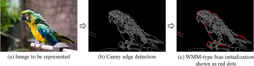
For 2D images, we approximate WMM location as edges of the image. Fig. 7 shows the flowchart for WMM-type initialization. We first start with the image to be represented and perform Canny edge dectection on it. We then use the binary edge map as a proxy for WMM locations. We then use the edge locations as bias values for each neuron in the Gabor INR.