Improved Forecasts of Global Extreme Marine Heatwaves Through a Physics-guided Data-driven Approach

In this study, we utilize two sets of reanalysis datasets of the ocean surface variables: the daily 1/4° eddy-permitting dataset and the 1/12° eddy-resolving dataset [Lellouche \BOthers. (\APACyear2018)]. The former is used to generate global eddy-permitting forecast, while the latter is for regional eddy-resolving forecast. Based on the different SST datasets, we conduct two experiments: one is the global 1/4° eddy-permitting MHW forecast, and the other is the North Pacific regional 1/12° eddy-resolving MHW forecast.

We utilize the \citeAhobday2016seasonal definition of MHW categories here. More precisely, any interval in which the SST anomalies surpass the 90th percentile for a minimum of five days in a row is classified as an MHW event. Subsequently, the MHWs are divided into three severity categories: moderate, strong, and severe/extreme. These categories are determined by the 90th, 92.5th, and 95th percentiles of the SSTA, respectively [Hobday \BOthers. (\APACyear2016)].

The atmospheric variables are obtained from ECWMF Reanalysis v5 (ERA5) [Hersbach \BOthers. (\APACyear2020)]. Based on the physical process, we select three variables: 10m wind components ($U_{{\rm 10}}$, $V_{{\rm 10}}$), 2m temperature ($T_{{\rm 2m}}$), and four surface heat flux variables (latent and sensible heat flux $Q_{{\rm lat}},Q_{{\rm sens}}$, shortwave and longwave radiation $Q_{{\rm SW}},Q_{{\rm LW}}$). The detailed description of the data can be found in Table 1:

Additionally, we are going to demonstrate the competitiveness of our forecasting framework against conventional numerical forecasting using GOFS 3.1 global ocean variable forecasting data, which is one of the leading numerical forecasts based on a 1/12° HYCOM model and NCODA system [Helber \BOthers. (\APACyear2013), Cummings (\APACyear2005), Cummings \BBA Smedstad (\APACyear2013)]. To facilitate comparison, we downsample the 1/12° resolution of the original data to 1/4°. In this study, we use data from 1993-2021 for a total of 29 years, with 1993-2017 as the training/validation set and 2018-2021 as the test set. All input variables mentioned above are normalized before they are fed into our model:

where the mean value and standard derivation are calculated over the training set.

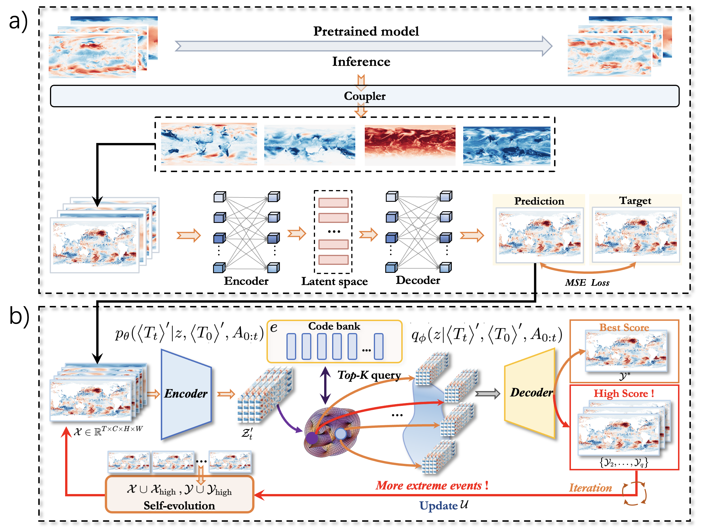
As shown in Figure 1, our model can be separated into two modules: the deterministic forecast module (Figure 1a) and the probabilistic data argumentation module (Figure 1b). The problem of marine heatwave forecast is essentially predicting the future state of mixed layer SSTA $\big{\langle}T_{t}\big{\rangle}^{\prime}$ based on the current state $\big{\langle}T_{0}\big{\rangle}^{\prime}$, here the brackets denote the average over the mixed layer and the prime is the deviation from the climatology mean. To be specific, we seek to approximate the evolution operator $\phi$:

In all, our goal is to use a neural network $\phi_{\theta}$ to approximate $\phi$ based on the existing data. The governing equation of $\big{\langle}T\big{\rangle}^{\prime}$ can be written as [Bian \BOthers. (\APACyear2023)]:

where u represents the horizontal velocity, and $Q_{{\rm SW}},Q_{{\rm LW}},Q_{{\rm sens}},Q_{{\rm lat}}$ is the shortwave radiation, longwave thermal radiation, sensible heat flux, and latent heat flux respectively. Integrate (3) we get

Guided by this physical nature of SSTA, we first use train a neural network (called a ‘coupler’) to approximate heat flux $Q^{\prime}=\phi_{\theta}^{(1)}(A_{0:t},\big{\langle}T_{0}\big{\rangle}^{\prime})$. Other effects, including advection and mixing effects, are approximated by another neural network $\big{\langle}T_{t}\big{\rangle}^{\prime}=\phi_{\theta}^{(2)}(Q^{\prime},\big{\langle}T_{0}\big{\rangle}^{\prime})$. In all, our framework can be expressed as:

In the training phase, the future atmosphere condition $A_{0:t}$ is the ground truth data from ERA5 while in the operational forecast, it’s replaced by the Pangu-weather’s forecast initialized by ERA ‘$t=0$’ analysis field [Bi \BOthers. (\APACyear2022)]. Furthermore, the AI-based Pangu-weather model only requires atmospheric variables as inputs, ensuring our framework’s self-consistency.

The specific structure of $\phi_{\theta}^{(1)}$ and $\phi_{\theta}^{(2)}$ is flexible and can be replaced with a variety of neural networks such as U-Net, SimVP, ConvLSTM, PastNet [Ronneberger \BOthers. (\APACyear2015), Gao \BOthers. (\APACyear2022), X. Shi \BOthers. (\APACyear2015), Wu \BOthers. (\APACyear2023)]. During the training and inference phase, the input variables is arrange into a 4-dimensional tensor $\mathcal{X}\in{\mathbb{R}}^{T*C*H*W}$, where $T=10$ is the forecast lead time, $C$ is the number of input variables, $(H,W)=(1440,720)$ (for eddy-permitting experiments) $(1200,300)$ (for eddy-resolving experiments) represents the horizontal resolution.

As pointed out in previous sections, overly smoothed forecast results will forbid AI-based model’s forecast ability on the most extreme MHW events. A key factor is that samples on extreme heatwaves are actually very scarce (less than $10\%$ by the definition of MHWs). Therefore, we need to generate more training samples with more extreme MHWs that conform to physical laws based on existing datasets, so as to improve the forecast ability of AI models in extreme events (i.e., data argumentation).

In numerical models, more forecast results can be obtained by ensemble forecasts. To be specific, under more realistic circumstances, small perturbations will be added to the initial value $\big{\langle}T_{0}\big{\rangle}^{\prime}$ and boundary condition $A_{0:t}$ due to the uncertainty in observation and subgrid scale signals. Thus, in actuality, $\big{\langle}T_{t}\big{\rangle}^{\prime}$ follows a particular probabilistic distribution $\big{\langle}T_{t}\big{\rangle}^{\prime}\sim p(\big{\langle}T_{t}\big{\rangle}^{\prime}|\big{\langle}T_{0}\big{\rangle}^{\prime},A_{0:t})$. In traditional numerical ensemble forecast, by adding perturbations that conform to certain patterns (for example, random noise or singular vectors), one can sample from this conditional distribution and boost the forecast ability.

Nevertheless, due to the fact that current AI-based models lack the chaotic effect [Selz \BBA Craig (\APACyear2023), L. Chen \BOthers. (\APACyear2024)], deep learning-based techniques cannot simply adopt the paradigm of adding initial perturbation. As a result, inspired by \citeAwu2024beamvq, rather than simply sample from the conditional distribution $p$, we utilized a vector quantised-variational autoencoder (VQVAE) to learn this distribution directly based on Bayesian theory [Van Den Oord \BOthers. (\APACyear2017)]. Specifically, our probabilistic approach consists of the following steps:

Step 1 : Pretrain the Deterministic Model. First, following section 2.2, we train a deterministic forecast model $\phi_{\theta}=\phi_{\theta}^{(1)}\circ\phi_{\theta}^{(2)}$ based on the existing training dataset $\{\mathcal{X}_{i}\}_{i=1}^{N}$ and model output $\{\mathcal{T}_{i}=\phi_{\theta}(\mathcal{X}_{i})\}_{i=1}^{N}$. However, as shown in Figure 4, those output is always overly smoothed due to the intrinsic deficiency of AI-based methods.

Step 2 : Learning the Conditional Distribution. Second, we use VQVAE to learn conditional distribution $p(\big{\langle}T_{t}\big{\rangle}^{\prime}|\big{\langle}T_{0}\big{\rangle}^{\prime},A_{0:t})$ (i.e., the distribution of SSTA $\big{\langle}T_{t}\big{\rangle}^{\prime}$ in the next 10 days, given the initial and boundary conditions). VQVAE model (abbreviated as $\Psi$) consists of two nerual networks: an encoder $q_{\phi}$ and a decoder $p_{\theta}$ (i.e., $\Psi=p_{\theta}\circ q_{\phi}$). In encoder, we want to transform the input $\big{\langle}T_{t}\big{\rangle}^{\prime}$ into a discrete latent space $\mathcal{Z}$. The latent representation is then fed to the decoder to reconstruct $\big{\langle}T_{t}\big{\rangle}^{\prime}$. As a result, Once the VQVAE is trained, we can simply sample in the $z\in\mathcal{Z}$ and use the decoder to acquire the conditional distribution $p$: $q_{\phi}(z)\sim p(\big{\langle}T_{t}\big{\rangle}^{\prime}|\big{\langle}T_{0}\big{\rangle}^{\prime},A_{0:t})$.

Mathematically, the role of encoder and decoder can be written as conditional distributions $q_{\phi}(z|\big{\langle}T_{t}\big{\rangle}^{\prime},\big{\langle}T_{0}\big{\rangle}^{\prime},A_{0:t})$ and $p_{\theta}(\big{\langle}T_{t}\big{\rangle}^{\prime}|z,\big{\langle}T_{0}\big{\rangle}^{\prime},A_{0:t})$. The goal of our model is to learn the distribution of $p$, that is, to minimize the ’distance’ between $q_{\phi}$ , $p_{\theta}$ and $p$. The former can be realized through minimizing the Kullback-Leibler Divergence (K-L Divergence, here we denote $X=(\big{\langle}T_{t}\big{\rangle}^{\prime},\big{\langle}T_{0}\big{\rangle}^{\prime},A_{0:t})$ for simplicity)

while the latter is equivalent to the maximize the maximum likelihood estimation ${\rm log}p_{\theta}$. As a result, the model is optimized through evidence lower bound (ELBO) $\mathcal{L}(q_{\phi},p_{\theta})$ of $p_{\theta}$ and $q_{\phi}$ to ensure the distribution of the output of $\Psi$ is as close as $p(\big{\langle}T_{t}\big{\rangle}^{\prime}|\big{\langle}T_{0}\big{\rangle}^{\prime},A_{0:t})$:

Where $D_{KL}$ is the K-L Divergence and $\mathbb{E}_{q_{\phi}}[{\rm log}p_{\theta}(\big{\langle}T_{t}\big{\rangle}^{\prime}|z,\big{\langle}T_{0}\big{\rangle}^{\prime},A_{0:t})]$ is the expectation of ${\rm log}p_{\theta}(\big{\langle}T_{t}\big{\rangle}^{\prime}|z,\big{\langle}T_{0}\big{\rangle}^{\prime},A_{0:t})$ under distribution $q_{\phi}$. Since $q_{\phi}(z|\big{\langle}T_{t}\big{\rangle}^{\prime},\big{\langle}T_{0}\big{\rangle}^{\prime},A_{0:t})$ in fact follows a discrete distribution, direct derivation shows that $\mathcal{L}$ is equivalent to the mean square error (MSE) loss (the K-L divergence term vanishes while the $\mathbb{E}_{z\sim q_{\phi}(z|X)}[{\rm log}p_{\theta}(\big{\langle}T_{t}\big{\rangle}^{\prime}|z,\big{\langle}T_{0}\big{\rangle}^{\prime},A_{0:t})]$ is equivalent to MSE loss):

In summary, based on the MSE loss, we can train the model to learn a more realistic distribution of $p$.

Step 3 : Data Augmentation Based on Forecast Ensembles. In this step, we are going to generate forecast ensembles from the learned distribution $p(\big{\langle}T_{t}\big{\rangle}^{\prime}|\big{\langle}T_{0}\big{\rangle}^{\prime},A_{0:t})$. To be specific, given the trained VQVAE model $\Psi=p_{\theta}\circ q_{\phi}$, $\{\phi_{\theta}(\mathcal{X}_{i})\}_{i=1}^{N}$ in step 1 with a Gaussian noise $z$ is input into encoder $q_{\phi}$ in order to generate latent representation $\{z_{i}\}_{i=1}^{N}$. Then, we perturb these latent representations by finding the top-$k$ closest for each input sample (in this study, we choose $k=10$):

where $||\bullet||$ is the Euclidean distance in the latent space. Those latent vectors is then fed into the decoder $p_{\theta}$ to generate the forecast ensembles $\mathcal{T}_{1}^{i},\mathcal{T}_{2}^{i},\ldots,\mathcal{T}_{k}^{i}$:

Since during the second step the trained decoder $p_{\theta}$ can already transform the latent representation $z\in\mathcal{Z}$ into the conditional distribution, those output forecast ensembles also follows the distribution $p(\big{\langle}T_{t}\big{\rangle}^{\prime}|\big{\langle}T_{0}\big{\rangle}^{\prime},A_{0:t})$ (i.e., more realistic SSTA fields under the initial and boundary conditions). In other words, by perturbing the latent representations, we acquire the forecast ensembles based on the deterministic forecast results.

Step 4 : Iterative Training Based on Data argumentation. Building upon the previous steps, in this step, we enhance the deterministic forecast model $\phi_{\theta}$ by incorporating high-quality samples generated from the learned conditional distribution $p$. Specifically, from the forecast ensembles ${\mathcal{T}_{1}^{i},\mathcal{T}_{2}^{i},\ldots,\mathcal{T}_{k}^{i}}$ generated in Step 3 for each input $\mathcal{X}_{i}$, we select a subset of $m$ high-quality samples ${\hat{\mathcal{T}}_{1}^{i},\hat{\mathcal{T}}_{2}^{i},\ldots,\hat{\mathcal{T}}_{m}^{i}}$ based on their proximity to the ground truth $\mathcal{T}_{i}^{\text{true}}$. The selection criterion is defined using the $L^{2}$ norm between the generated samples and the ground truth:

The formula above is calculated for all grid points where MHW events occur. These selected high-quality samples are then combined with the original dataset to form an augmented training set:

We then retrain the deterministic model $\phi_{\theta}$ on the augmented dataset $\mathcal{D}_{\text{aug}}$ to improve its forecasting performance. The loss function for retraining is defined as:

This retraining process leverages both the original ground truth and the high-quality generated samples to refine the model. By incorporating the selected samples that closely resemble the ground truth, the model learns to better capture the variability and extremes present in the data.

In summary, this approach not only enhances the deterministic model’s performance but also mitigates the over-smoothing issue observed in AI-based forecasting methods.

In this study, to evaluate the performance of our model, we use three metrics: Root Mean Square Error (RMSE), Critical Success Index (CSI) and Symmetric Extremal Dependence Index (SEDI). RMSE represents the overall performance of our SST anomaly forecast, which is calculated as:

Where $T_{i,j}(t)$ and $\tilde{T}_{i,j}(t)$ is the ground-truth and prediction of SST anomaly at lead time $t$. The subscript $(i,j)$ indicates the data at grid point $(i,j)$ while H and W follows the same definition in section 2.1. CSI and SEDI are the metrics that evaluate the forecast ability of extreme events and can be expressed as:

and

Where TP (True Positive) denotes the number of cases that a MHWs event is accurately predicted. FP (False Positive), FN (False Negative), and TN (True Positive) follow a similar definition. $F=\frac{FP}{FP+TP}$ is the false alarm rate while $H=\frac{TP}{TP+FN}$ is the hit rate.

In this study, we also utilize explainable AI (XAI) method to evalute the relative importance of each input of our model $\phi_{\theta}$. To be specific, by removing the $i^{\rm{th}}$ variables from our input, we can quantitatively measure the (unsigned) contribution of each variable on the heat flux (called ‘contribution map’) at grid point $(m,n)$, which is calculated as:

The signed contribution can be calculate as:

Where $\{\mathcal{X}_{i}\}_{i=1}^{N}$ is the full input variables while $\{\mathcal{X}_{i}^{j}\}_{i=1}^{N}$ is the modified input with the $j^{\rm{th}}$ element replaced with zero. $Y$ represents the all MHW events and $|Y|$ is the number of MHW events. Similar approaches can be found at [Shin \BOthers. (\APACyear2022), Shin \BOthers. (\APACyear2024), Lyu \BOthers. (\APACyear2023)].

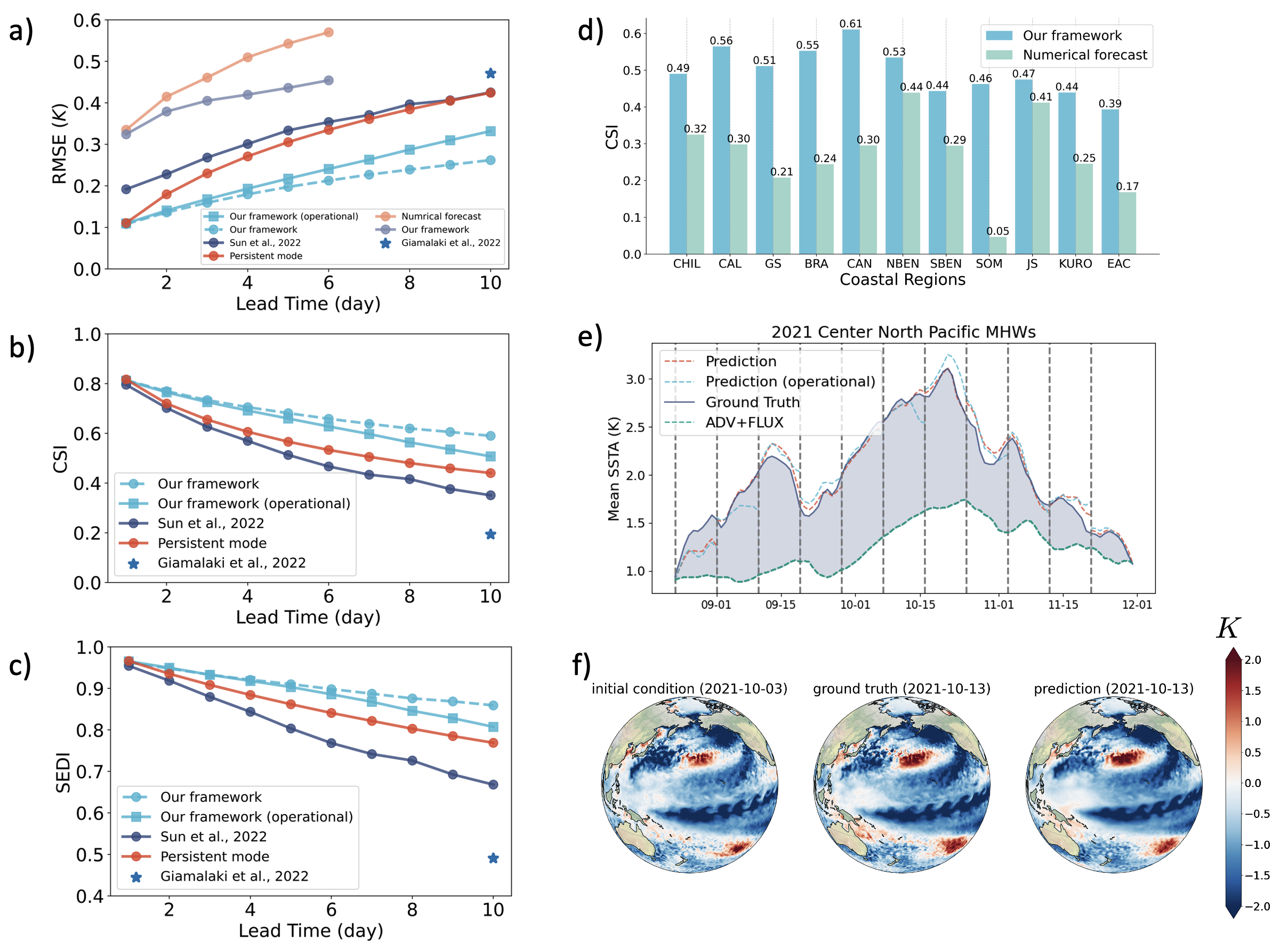
Figure 2 illustrates the performance of our framework in the global 1/4° dataset. Overall, our framework’s forecasting ability for $\big{\langle}T\big{\rangle}^{\prime}$ exceeds existing data-driven models [Giamalaki \BOthers. (\APACyear2022), W. Sun \BOthers. (\APACyear2023)], and the mean RMSE of 10-day forecast can be reduced by $30\%$ to $40\%$. In addition, our framework has shown to be quite competitive compared to numerical models. Since there is a certain deviation of SST in different sources of observation or analysis data, in this study, we use GOFS’s analysis field as the input initial condition of the model to ensure the fairness of the comparison. However, despite the unfavorable conditions for our framework, our model’s 6-day forecast RMSE is still $20\%$ to $30\%$ lower than that of the numerical model. What’s more, as shown in Figure 2a, the boundary condition $A_{0:t}$ plays an important role in the forecasting of $\big{\langle}T\big{\rangle}^{\prime}$. Under a realistic operational forecast condition, the $A_{0:t}$ is replaced by the predicition of Pangu-weather, which will impair the forecast ability of $\big{\langle}T\big{\rangle}^{\prime}$ (with the RMSE increasing about $20\%$, see the solid and dash blue line in Figure 2a). In other words, as the lead time marches on, the accuracy of the estimation of the atmospheric condition $A_{0:t}$ has an increasing impact on our framework.

What’s more, when it comes to the extreme SSTA events (i.e., marine heatwaves), our model has also shown good forecasting capabilities. Figure 2b-2c shows the global average for CSI and SEDI indicators. Comparing to the existing data-driven methods, our model also significantly improves the ability to capture such MHWs. Coastal ecosystems are the richest and most complex in the ocean [Costello \BBA Chaudhary (\APACyear2017), Halpern \BOthers. (\APACyear2008)]. In this study, we also evaluate the forecast skills of coastal MHWs against the numerical model over 11 coastal regions following \citeAmarin2021slower (Figure 2d). There is a $20\%$ to $50\%$ improvement in CSI of each region, especially along the coastline of Somalia (SOM) where numerical model can only capture a small portion of MHW events. This provided a potential application of our model to coastal MHWs forecast.

We also evaluate our framework’s forecast ability in well-known, long-persisting extreme MHWs events. For example, within the Central North Pacific region, strong MHWs are frequently observed during 2019-2021 summer (Abbreviated as CNP-MHW in the following paragraphs). Here we take 2021 CNP-MHW as an example, as shown in Figure 2e-2f. More examples can be found in Figure S2. Based on the heat budget equations (3), the ‘surface effects’, including the advection (ADV) and heat flux (FLUX) term, can only explain about $30\%$ of the total changes of SSTA during the intensifying and decaying phase of CNP-MHW as in Figure 2e. In fact, based on Argo profiling data, \citeAnishihira2024record found that during 2021 Summer, the Central Mode Water (CMW) decreased extremely, leading to less cooling heat flux associated with the entrainment of subsurface waters into mixed layer, which contributed to form the CNP-MHW. This means that after receiving the FLUX term from coupler $\phi_{\theta}^{(1)}$, our main model $\phi_{\theta}^{(2)}$ can parameterize the subsurface mixed layer entrainment process based on the surface data. Overall, our approach has the potential capacity to replicate the subsurface process from surface data, demonstrating our model’s robustness under more complex MHW patterns.

In addition to the high accuracy of MHWs forecasting, our framework also significantly improves the efficiency. To be specific, our model only takes 0.2 seconds to complete a 10-day global MHW forecast on a single A100 GPU, which is several orders of magnitude faster than numerical forecast systems [Bi \BOthers. (\APACyear2022), Wang \BOthers. (\APACyear2024)].

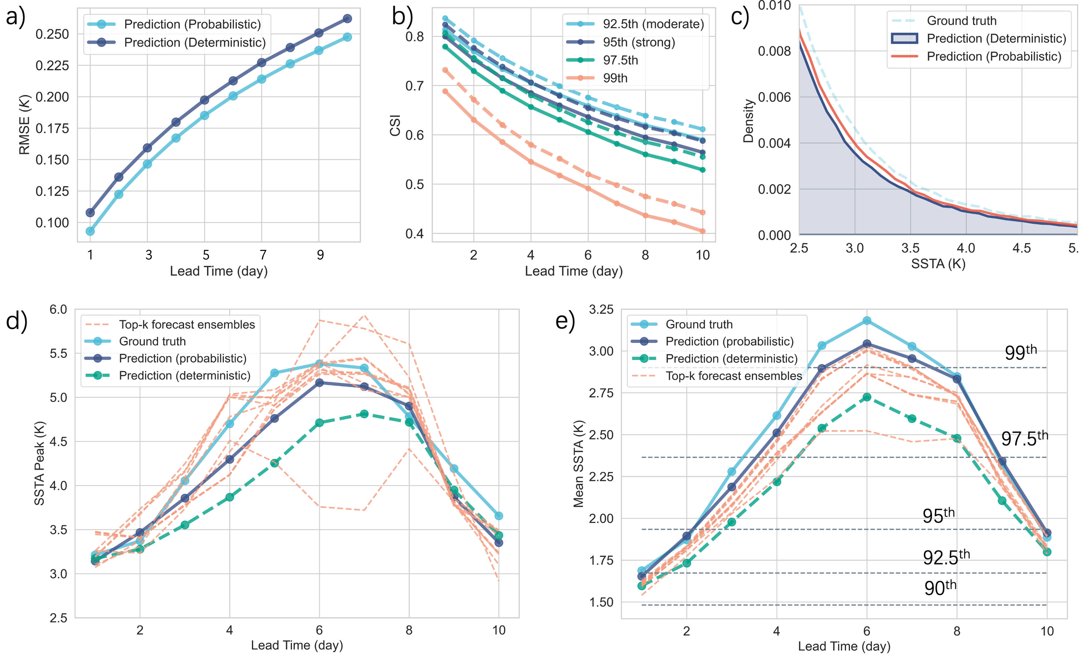
Unlike numerical models or large-AI driven ocean model that treats the SST as a primitive variable, we are more concerned with capturing the extremes of the SST. In this study, we apply the probabilistic method in section 2.3 to our deterministic forecasting, which effectively improves the overall forecasting ability of the framework and extreme MHWs. To be more explicit, as demonstrated in Figures 3a-3b, after incorporating the probabilistic module, all of the metrics steadily improve. Even in the most intense MHWs incidents (99th percentile), the CSI still increases by approximately $15\%$.

Here we used the CNP-MHW in 2020 (as mentioned in section 3.1) to illustrate how our forecast ensembles improves the forecast ability of extreme events (we don’t take 2021 CNP-MHW mainly because the backbone module can already generate satisfying result). Figure 3d shows a 10-day forecast of the CNP-MHW event initialized at 2020-08-14 and ending at 2020-08-24. The level of CNP-MHW gradually rose from moderate to extreme, broke the $99\%$ threshold on 2020-08-19, and then steadily declined. Our deterministic forecasting framework can also capture the formation of CNP-MHW, but it is significantly underestimated in intensity. Using the probabilistic model mentioned in Section 2.3, we sampled $k=10$ forecast ensembles from the conditional distribution $p(\big{\langle}T_{t}\big{\rangle}^{\prime}|\big{\langle}T_{0}\big{\rangle}^{\prime},A_{0:t})$ and added them to the training samples. It can be found that most of the 10 forecast ensembles capture extreme temperature enhancements, and their intensity is higher than that of the deterministic model, which is closer to the real situation. As a result, the new forecasting model trained on the enhanced forecast ensembles dataset can accurately capture the CP-MHW enhancement process and improve the prediction ability of extreme heat waves. A similar analysis is performed on the peak value of $\big{\langle}T_{t}\big{\rangle}^{\prime}$, which leads to a similar conclusion.

Adding those new forecast ensembles allows the dataset to be more widely distributed, allowing our forecast model to capture out-of-distribution MHW events, which can also be verified by Figure 3c. By calculating the probability density function (PDF) of $\big{\langle}T_{t}\big{\rangle}^{\prime}$, we find that the new probabilistic forecast model can lead to more extreme MHW events than conservative estimates based on deterministic forecast. In another word, our probabilistic-based data argumentation serves as a distribution shift that pulls the conservative and over-smoothing forecast back to more extreme and rare cases.

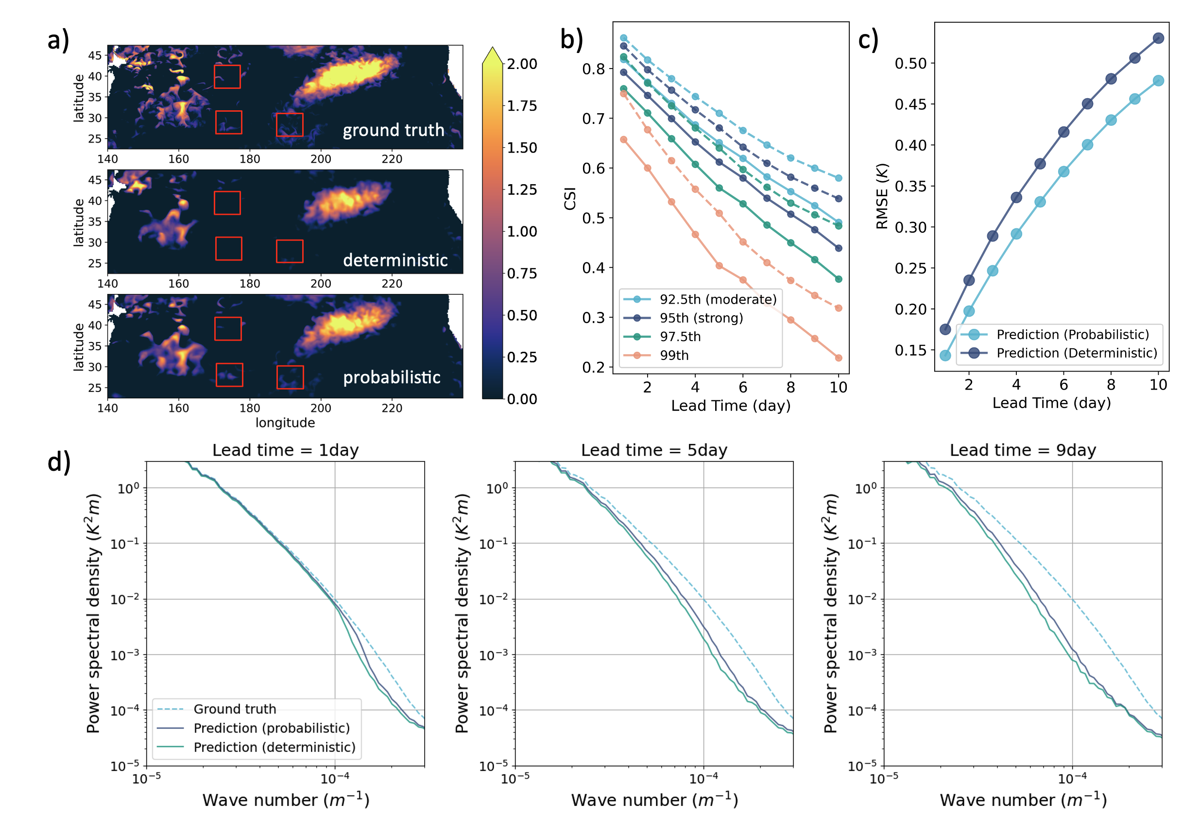
Another question is about our framework’s performance in the eddy-resolving regime. As pointed out by \citeAbian2023oceanic,bian2024scale, as the resolution increases, more small-scale MHWs will occur with life cycles of about 5-10 days. These MHWs are always small at spatial scale (around the first baroclinic Rossby deformation radius) and are mainly driven by mesoscale-induced local advection. An example can be found in Figure 4a, marked within the red boxes. As shown in the figure, in the deterministic forecast, although it can accurately forecast the emergence of the 2020 Northeast Pacific MHWs, many small structures of MHWs are ignored. However, enhanced by probabilistic model-based forecast ensembles, the small-scale MHW structures in the red boxes can be predicted with accurate intensity and shape. To further illustrate this multi-scale forecast issue, we also conduct a more detailed analysis based on the power spectrum of SSTA ground truth and forecast at different lead times in Figure 4d. Generally speaking, due to the overly smoothing issues in AI methods, our deterministic model shows a weaker SSTA spectrum at the mesoscale regime (corresponding to wave number about $10^{-4}m^{-1}$). At a shorter time scale (1 day), the improvement of the probabilistic model is mainly reflected in the strengthening of the mesoscale MHW structure. As the forecast lead time marches on, our probabilistic model is more inclined to improve MHWs forecast at a larger scale. In all, our probabilistic model can improve the model’s ability to predict the structure of small-scale MHWs, which shows potential applications in regional forecasting.

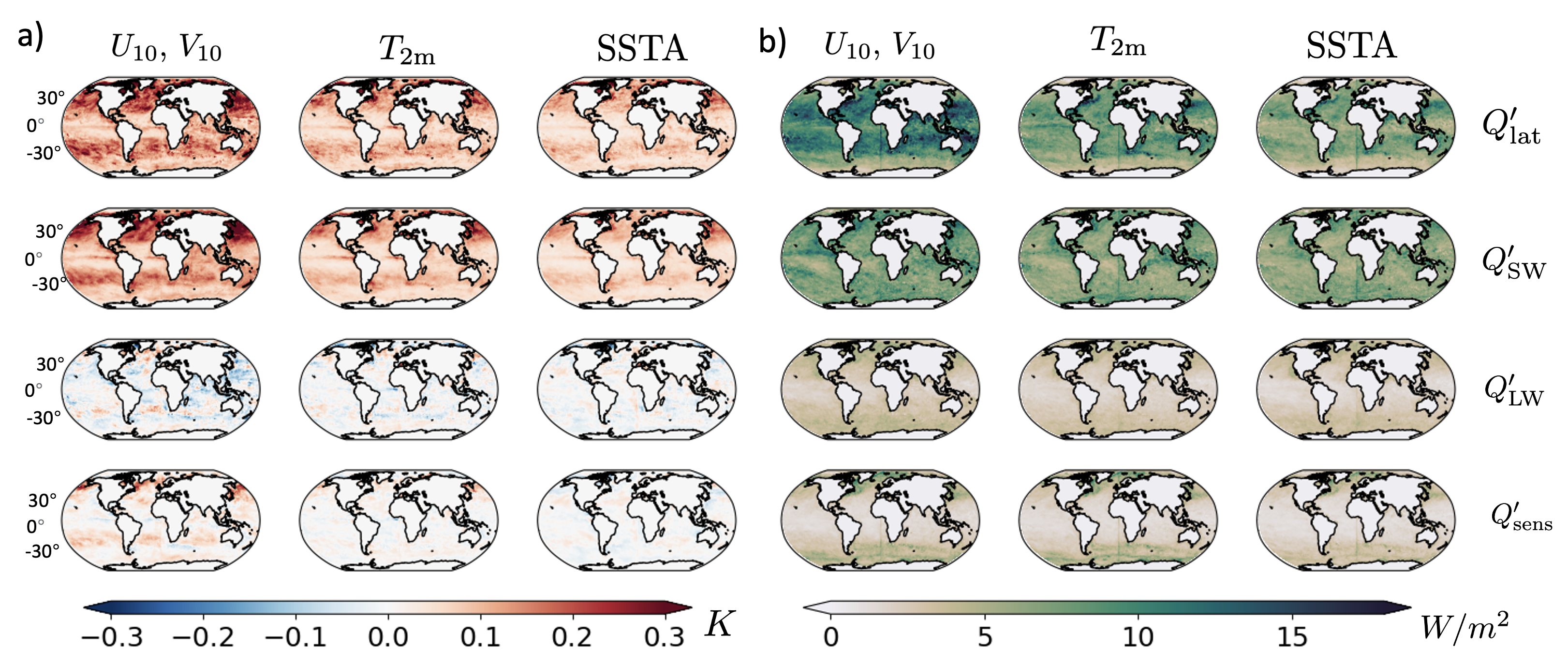
In this section, we are going to focus on the explainability of our framework. In other words, we want to determine the key factors that drive the small-scale variations (10-day) of MHWs through the signed and unsigned contribution map described in section 2.4. By averaging equations (17) and (18) over the decaying and intensifying phase of MHWs, we can quantify the role of each input variables in the life cycle of MHWs, as illustrated in Figure 5.

First we examine the contribution map of each input variable on the SSTA variations during intensifying/decaying phase of MHWs (i.e., the output of $\phi^{(2)}_{\theta}\circ\phi^{(1)}_{\theta}$). As shown in Figure 5a, the contribution of surface wind speed is the largest among each variable, which leads to a maximum about $0.3$ K deviation of SSTA in both the intensifying and decaying phases. The surface temperature follows the wind speed and the contribution of SSTA is the smallest. The unsigned contribution of atmosphere and ocean variables is mainly concentrated in midlatitude and subarctic regions (e.g., Northeast Pacific and Western Boundary Currents). When considering the signed contribution, removing surface wind speed will generally lead to an underestimate in both intensifying and decaying phase of MHWs. This further emphasize the wind speed as a important predictor in the most extreme MHWs events.

When considering the contribution of inputs on each flux given by coupler (i.e. the output of $\phi^{(1)}_{\theta}$, Figure 5b), the contribution map still proves the surface wind speed as the key driving factor. More specifically, the contribution of surface wind on latent heat flux is the largest, where $\Delta C^{ns}_{j}$ is mainly confined within the subtropical regions, with peak values are found in the East Pacific and Western Australia. The influence on short-wave radiation is also relatively considerable, followed by sensible heat flux, and long-wave radiation is the least affected. In addition, large response of heat flux can be found along Western Boundary Currents, such as the Gulf Stream, Kuroshio Extension, and Agulhas System. Along these regions, eddy activities can feedback to the atmosphere, which will further maintain or strengthen the MHWs through air-sea heat flux [Holbrook \BOthers. (\APACyear2019)].

However, as mentioned above, the spatial distribution of input variables on SSTA and air-sea heat flux is quite different, especially in the Northern Hemisphere (including the well-known Northeast Pacific MHWs). According to (3), the relatively deep mixed layer in the midlatitudes should reduce the response of MHWs to the same heat flux change. This contradiction indicates that the small-scale variations of MHWs in the midlatitude ocean is more sensitive to the changes in the heat flux. We hypothesize that it may be due to the intricate subsurface effect that drives the amplifying of MHWs in these regions. For example, the subsurface entrainment process is believed to drive the Central North Pacific MHWs, while the anomalous mixed layer depth can contribute to Northeast Pacific MHWs [Nishihira \BBA Sugimoto (\APACyear2024), J. Shi \BOthers. (\APACyear2022)]. In summary, in our framework, the surface wind speed is the key factor of the predictability of MHWs, which mainly controls the development of MHWs by affecting surface latent heat flux.