Improved measurements of and
Abstract
Using 7.93 fb-1 of collision data collected at the center-of-mass energy of 3.773 GeV with the BESIII detector, we measure the absolute branching fractions of , , , and to be , , , and , respectively. By performing a simultaneous fit to the partial decay rates of these four decays, the product of the hadronic form factor and the modulus of the CKM matrix element is determined to be . Taking the value of from the standard model global fit or that of from the LQCD calculation as input, we derive the results and .
I Introduction
Improved measurements of semileptonic decays of charmed mesons provide important inputs to further the understanding of weak and strong interactions in the charm sector. By analyzing their decay dynamics, one can determine the product of the modulus of the Cabibbo-Kobayashi-Maskawa (CKM) matrix element and the hadronic transition form factor. Taking as an example, the hadronic transition form factors at zero-momentum transfer Lubicz:2017syv ; Chakraborty:2021qav ; Parrott:2022rgu ; FermilabLattice:2022gku ; Wu:2006rd ; Verma:2011yw ; Ivanov:2019nqd ; Faustov:2019mqr ; Ke:2023qzc can be calculated via several theoretical approaches, e.g., lattice quantum chromodynamics (LQCD) Lubicz:2017syv ; Chakraborty:2021qav ; Parrott:2022rgu ; FermilabLattice:2022gku , QCD light-cone sum rules (LCSR) Wu:2006rd , covariant light-front quark model (LFQM)Verma:2011yw , the covariant confined quark model (CCQM) Ivanov:2019nqd , and the relativistic quark model (RQM) Faustov:2019mqr . Using the value of provided by the CKMFitter group pdg2022 , the hadronic transition form factor can be calculated, resulting in a stringent test of the theoretical predictions. Conversely, using the value predicted by theory allows the determination of , which is important to test CKM matrix unitarity. Furthermore, measurements of the branching fractions of and ( or ) are important to test lepton flavor universality and isospin conservation in .
Previously, the branching fractions of and were measured by BESII BES:2004rav ; BES:2004obp ; BES:2006kzp , BaBar BaBar:2007zgf , Belle Belle:2006idb , CLEO-c CLEO:2005rxg ; CLEO:2005cuk ; CLEO:2007ntr ; CLEO:2009svp , and BESIII BESIII:2021mfl ; BESIII:2015tql ; BESIII:2018ccy ; BESIII:2017ylw ; BESIII:2016hko ; BESIII:2015jmz ; BESIII:2016gbw . Studies of the decay dynamics of were reported by BaBar BaBar:2007zgf , CLEO-c CLEO:2009svp , and BESIII BESIII:2015tql ; BESIII:2018ccy ; BESIII:2017ylw ; BESIII:2015jmz . The previous BESIII analysis used 2.93 fb-1 of collision data taken at the center-of-mass energy GeV. This paper reports improved measurements of the branching fractions and decay dynamics of and by using 7.93 fb-1 of collision data collected by the BESIII detector at GeV Luminosity . Throughout this paper, charge conjugate modes are implied.
II BESIII detector and Monte Carlo simulations
The BESIII detector Ablikim:2009aa records symmetric collisions provided by the BEPCII storage ring Yu:IPAC2016-TUYA01 in the center-of-mass energy range from 1.84 to 4.95 GeV, with a peak luminosity of achieved at . BESIII has collected large data samples in this energy region Ablikim:2019hff ; Li:2021iwf . The cylindrical core of the BESIII detector covers 93% of the full solid angle and consists of a helium-based multilayer drift chamber (MDC), a time-of-flight system (TOF), and a CsI(Tl) electromagnetic calorimeter (EMC), which are all enclosed in a superconducting solenoidal magnet providing a 1.0 T magnetic field. The solenoid is supported by an octagonal flux-return yoke with resistive plate muon identification counters (MUC) interleaved with steel. The main function of the MUC is to separate muons from charged pions, other hadrons and backgrounds based on their hit patterns in the instrumented flux-return yoke. The charged-particle momentum resolution at is , and the resolution is for electrons from Bhabha scattering. The EMC measures photon energies with a resolution of () at GeV in the barrel (end-cap) region. The time resolution in the plastic scintillator TOF barrel region is 68 ps, while that in the end-cap region was 110 ps. The end-cap TOF system was upgraded in 2015 using multi-gap resistive plate chamber technology, providing a time resolution of 60 ps etof . Approximately 67% of the data used here was collected after this upgrade.
Simulated samples produced with geant4-based geant4 Monte Carlo (MC) software, which includes the geometric description Huang:2022wuo of the BESIII detector and the detector response, are used to determine detection efficiencies and to estimate backgrounds. The simulation models the beam energy spread and initial state radiation (ISR) in the annihilations with the generator kkmc ref:kkmc . Signal MC samples of the decays are simulated with a specific two-parameter series expansion model Becher:2005bg . The background is studied using an inclusive MC sample that consists of the production of pairs from the (including quantum coherence for the neutral channels), the non- decays of the , the ISR production of the charmonium states, and the continuum processes. These processes are also generated with kkmc. The known decay modes are modeled by evtgen ref:evtgen with branching fractions taken from the Particle Data Group (PDG) pdg2022 , while the remaining unknown charmonium decays are modeled with lundcharm ref:lundcharm . Final state radiation from charged final-state particles is incorporated using photos photos .
III Measurement Method
At GeV, the and mesons are produced in pairs from the process, where stands for or . This property allows us to do absolute branching fraction measurement with the well established double-tag (DT) method DTmethod . In this method, the single-tag (ST) candidate events are selected by reconstructing a in the six hadronic final states , , , , , and , or a in the six hadronic final states , , , , , and . These inclusively selected candidates are referred to as ST mesons. In the presence of the ST mesons, candidates for the signal decays are selected to form DT events. The branching fraction of the signal decay is determined by
| (1) |
where is the total DT yield in data, is the total ST yield
| (2) |
where is the ST yield of tag mode , and is the weighted efficiency of detecting the semileptonic decay, calculated by
| (3) |
Here, , is the efficiency of detecting the semileptonic decay in the presence of the ST meson of tag mode , where and are the DT efficiency and ST efficiency, respectively.
IV Selection of single tag mesons
For each charged track (except for those used for reconstruction), the polar angle () with respect to the MDC axis is required to satisfy , and the point of closest approach to the interaction point must be within 1 cm in the plane perpendicular to the MDC axis, , and within 10 cm along the MDC axis, . Charged tracks are identified by using the and TOF information, with which the combined confidence levels under the pion and kaon hypotheses are computed separately. Charged tracks are assigned to the particle type that has the higher probability.
Candidate mesons are reconstructed from pairs of oppositely charged tracks. For these two tracks, their polar angles are required to satisfy and the distance of closest approach to the interaction point is required to be less than 20 cm along the MDC axis. There is no requirement on the distance of closest approach in the transverse plane, and no particle identification (PID) criteria are required. The two charged tracks are constrained to originate from the same vertex, which is required to be away from the interaction point by a flight distance of at least twice the vertex resolution. The quality of the vertex fit is ensured by the requirement of , and the invariant mass of the pair is required to be within GeV/.
Neutral pion candidates are reconstructed via the decay. Photon candidates are identified from EMC showers. The EMC time difference from the event start time is required to be within ns. The energy deposited in the EMC is required to be greater than 25 MeV in the barrel region () and 50 MeV in the end-cap region (). The opening angle between the photon candidate and the nearest charged track in the EMC is required to be greater than . For any candidate, the invariant mass of the photon pair is required to be within GeV. To improve the momentum resolution, a mass-constrained (1C) fit to the known mass pdg2022 is imposed on the photon pair, and the of the 1C kinematic fit is required to be less than 50. The four-momentum of the candidate from this kinematic fit is used for further analysis.
For the two-body tag mode of , the backgrounds originating from cosmic rays, Bhabha and dimuon events are vetoed with the following procedure defined in Ref. deltakpi . It is required that the TOF time difference between the two charged tracks is less than 5 ns, and at least one EMC shower with energy greater than 50 MeV or at least one additional charged track detected in the MDC survives in each event. Further, it is required that the two charged tracks are not consistent with being a muon pair or an electron-positron pair, identified using the TOF, , EMC, and MUC measurement information with the combined confidence levels , , , and for electron, muon, kaon, and pion hypotheses, respectively. To be identified as an electron, is required to be greater than 0 and larger than , , as well as . To identify a track as a muon, is required to be greater than 0, the deposited energy in the EMC should fall within the range of 0.15 to 0.30 GeV, and the hit depth in the MUC needs to be either greater than cm or greater than 40 cm, where is the track momentum.
To identify the ST mesons, we use two kinematic variables: the energy difference and the beam-constrained mass , where is the beam energy, and and are the total energy and momentum of the ST meson in the center-of-mass frame, respectively. If there are multiple candidates for a specific tag mode, the one giving the least is chosen for further analysis. To suppress combinatorial backgrounds in the distribution, tag dependent requirements are imposed on the ST candidates. The detailed requirements and the ST efficiencies estimated by analyzing the inclusive MC sample are summarized in Table 1.
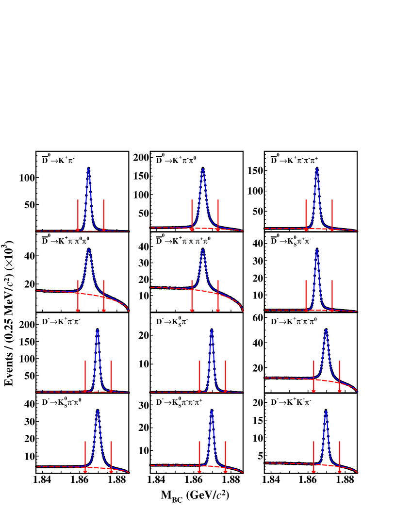
For each tag mode, the yield of ST mesons is obtained by the maximum likelihood fit to the corresponding distribution. In the fit, the signal shape is described by the sum of an MC-simulated signal shape, made by RooHistPdf in Rootclass RootClass , convolved with a double-Gaussian resolution function plus a single-Gaussian function, to account for resolution difference between data and MC simulation and initial state radiation (ISR) effects. The parameters of those functions are free. The background shape is described by an ARGUS function argus with the endpoint fixed at the value. Figure 1 shows the results of the fits to the distributions of the accepted ST candidates in data for different tag modes. The candidates with within GeV/ for tags and GeV/ for tags are kept for further analysis. Summing over the tag modes gives the total yields of ST and mesons () to be and , respectively.
| Tag mode | (MeV) | |||
|---|---|---|---|---|
V Selection of double tag events
The candidates for , , , and are selected from the remaining tracks in the presence of the ST candidates. Candidates for and are selected with the same criteria as those used in the ST selection. The positron and muon are identified using the TOF, , and EMC measurements with the combined confidence levels , , , and , which are calculated for electron, muon, kaon, and pion hypotheses, respectively. The positron candidate is required to satisfy and . The muon candidate is required to satisfy and , and the energy of the muon deposited in the EMC is required to be within GeV.
To suppress backgrounds associated with hadronic decays, it is required that there are no additional good charged tracks on the signal side (). To reject the backgrounds from hadronic decays involving , the maximum energy of extra photons () not used in the event reconstruction is required to be less than 0.25 GeV. Requirements on the and () invariant mass, which are GeV/ for , GeV/ for , GeV/ for , and GeV/ for , are used to suppress the backgrounds associated with the misidentification between and .
The neutrino is not detectable by the BESIII detector. In order to determine the number of semileptonic candidates, we define , where and are the missing energy and momentum of a DT event in the center-of-mass frame, respectively. They are calculated by and , where and are the measured energy and momentum of the candidate in an event. Here to improve the resolution, is evaluated as , where is the unit vector in the momentum direction of the ST meson and is the known mass pdg2022 .
VI Branching fractions
VI.1 Results on branching fractions
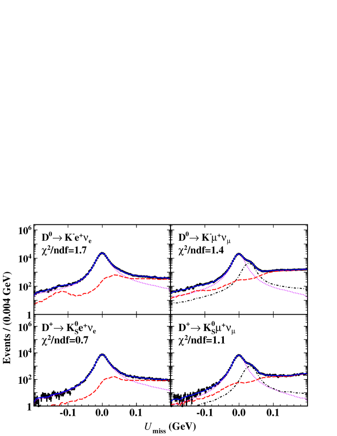
After imposing all selection criteria, the distributions of the accepted candidates for in data are shown in Fig. 2. Studies of the inclusive MC sample show that main backgrounds are caused mainly due to mis-identifying or as for channels; mis-identifying as for channels; or missing (s) for all signal decays. The main sources of backgrounds, normalized yields and fractions, which are estimated from the inclusive MC sample, are listed in Table 2.
For each signal decay, the signal yields in data are obtained from the maximum likelihood fits to the corresponding distributions. In the fit, the signal shape is determined from the simulated shape convolved with a Gaussian function with free parameters, which accounts for different resolutions between data and MC simulation. For the decays, the main peaking backgrounds are modeled by the simulated shapes convolved with the same Gaussian function as the corresponding signal, and their yields are free. In the distributions, there are also small peaking backgrounds from around 0.03 GeV for , and small peaking background around GeV for . Their shapes and yields are fixed in the fits and merged into other backgrounds in the plots. The shapes of signal and all backgrounds are derived from signal and inclusive MC samples, respectively, and all of them are made by RooHistPdf in Rootclass RootClass . From these fits, we obtain the signal yields of each signal decay in data ().
The DT efficiencies are obtained by analyzing the corresponding signal MC samples. The obtained DT efficiencies and signal efficiencies for different signal decays in each tag mode as well as the weighted signal efficiencies () are listed in Table 3.
| Signal decay | Background source | ||
| 9820 | 46.7 | ||
| 5421 | 25.8 | ||
| 2756 | 13.1 | ||
| 458 | 2.2 | ||
| 44932 | 44.2 | ||
| 28815 | 28.3 | ||
| 8285 | 8.2 | ||
| 2821 | 51.6 | ||
| 1558 | 28.5 | ||
| 261 | 4.8 | ||
| 8760 | 50.3 | ||
| 2546 | 14.6 | ||
| 2072 | 11.9 |
| decay | decay | ||||||||
|---|---|---|---|---|---|---|---|---|---|
| Tag mode | Tag mode | ||||||||
With the signal yields in data , the weighted signal efficiencies , as well as the ST yield in data, the branching fractions of , , , and are determined with Eq. (1) and listed in Table 4.
| Signal decay | |||
|---|---|---|---|
VI.2 Systematic uncertainties on branching fractions
Table 5 summarizes the sources of the systematic uncertainties in the branching fraction measurements. They are assigned relative to the measured branching fractions and are discussed below.
ST yields
The systematic uncertainty of the fits to the spectra is estimated by varying the signal and background shapes and repeating the fits for both data and the inclusive MC sample. A variation of the signal shape is obtained by modifying the matching requirement between generated and reconstructed angles from 15∘ to 10∘ or 20∘. The uncertainty related to the background shape is obtained by varying the endpoint by MeV. In addition, the effect of removing the requirements from the ST selection is evaluated, and the difference with the nominal measurement is taken as a systematic uncertainty accounting for possible mismodelling of the distribution in simulation. Adding these three effects quadratically leads to a 0.3% variation, which is taken as the systematic uncertainty on . The uncertainty in the ST yield is correlated for and , while that for the ST yield is correlated for and .
tracking and PID
The tracking and PID efficiencies are studied by using a control sample of hadronic events, with decaying into , and decaying into , , as well as decaying into and decaying into . The ratios of the momentum weighted data and MC efficiencies are and for tracking and PID, respectively. The signal efficiencies are corrected by these ratios, and their uncertainties, which are correlated for and , are assigned as systematic uncertainties.
reconstruction
The reconstruction efficiencies are examined in two aspects. The tracking efficiencies are determined by using the control samples used in the studies of tracking and PID, but with a missing . The efficiencies associated with the mass window and decay vertex fit are examined using the hadronic events, with or decaying into , , , , , and . The polar angle distribution of the control sample is consistent with that in the signal decays, therefore its effect on the reconstruction efficiency is negligible. The momentum weighted difference between the reconstruction efficiency of data and MC is 0.84% for and 0.88% for , which are taken as the systematic uncertainties. These uncertainties are correlated for and .
tracking and PID
The tracking and PID efficiencies of and are studied by using the control samples of and , respectively. The ratios of the data and MC efficiencies weighted by momentum and cos are for tracking and for PID; while they are for tracking and for PID. The signal efficiencies are corrected by these factors. After correction, the uncertainties of ratios are assigned as the systematic uncertainties, and these uncertainties are correlated for the four signal decays.
MC model
The detection efficiencies are estimated by using signal MC events generated with the hadronic transition form factors measured in this work. The corresponding systematic uncertainties are estimated by varying the parameters by . These uncertainties are independent for each signal decay.
requirement
The uncertainty due to the upper bound in each signal decay is studied by scanning the requirement from 1.74-1.84 GeV/ for semielectronic decay and 1.46-1.56 GeV/ for semimuonic decay with a step of 0.01 GeV. We find the changes of branching fractions are smaller than the statistical uncertainty difference . Therefore, we neglect this systematic uncertainty.
and requirements
The systematic uncertainty of the and requirements is estimated by control samples of hadronic events, with both and decaying into one of the used ST hadronic final sates. The difference of the acceptance efficiencies between data and MC simulation is assigned as the systematic uncertainty. These uncertainties are correlated for and or and .
fit
The systematic uncertainty due to the fit is considered in two parts. Since a Gaussian function is convolved with the simulated signal shapes to account for the resolution difference between data and MC simulation, the systematic uncertainty from the signal shape is ignored. The systematic uncertainty due to the background shape is assigned by varying the relative fractions of backgrounds from and the dominant background channels in the inclusive MC sample within the uncertainties of their input branching fractions. The changes in the branching fractions are taken as the corresponding systematic uncertainties. These uncertainties are independent for the four signal decays.
MC statistics
The relative uncertainties on the signal efficiencies are assigned as systematic uncertainties due to MC statistics. These uncertainties are independent for the four signal decays.
Quoted branching fractions
For the and decays, the uncertainty of the quoted branching fraction of is 0.07% pdg2022 . These uncertainties are correlated for and .
| Source | ||||
|---|---|---|---|---|
| 0.30 | 0.30 | 0.30 | 0.30 | |
| tracking | 0.10 | 0.10 | – | – |
| PID | 0.10 | 0.10 | – | – |
| reconstruction | – | – | 0.85 | 0.89 |
| tracking | 0.10 | 0.10 | 0.10 | 0.10 |
| PID | 0.10 | 0.16 | 0.10 | 0.15 |
| MC model | 0.20 | 0.19 | 0.10 | 0.05 |
| requirement | – | – | – | – |
| and requirement | 0.10 | 0.10 | 0.10 | 0.10 |
| fit | 0.18 | 0.14 | 0.06 | 0.05 |
| MC statistics | 0.05 | 0.06 | 0.07 | 0.07 |
| Quoted branching fractions | – | – | 0.07 | 0.07 |
| Total | 0.46 | 0.46 | 0.93 | 0.97 |
VII Hadronic transition form factors
VII.1 Theoretical formula
The differential decay width of the semileptonic decay can be expressed as Faustov:2019mqr
| (4) |
where is the four-momentum transfer to the system, is the modulus of the meson three-momentum in the rest frame, is the Fermi constant, is the vector form factor, and is the scaler form factor. The series expansion Becher:2005bg is the most popular parameterization to describe the hadronic transition form factor, which has the form
| (5) |
Here, are the real coefficients, and , where . The function is given by
| (6) |
where , , and are the masses of and particles, is the pole mass of the vector form factor accounting for the strong interaction between and mesons and usually taken as the mass of the lowest lying vector meson , which is 2112.2 MeV pdg2022 . The parameter is obtained from dispersion relations using perturbative QCD chiV ,
| (7) |
where GeV is the -quark mass.
In this analyses, the two-parameter series expansion is enough to describe the data, i.e.
| (8) |
By setting , the vector form factor can be written as
| (9) |
The scalar form factor is similar to but with a one-parameter series expansion, which is given by Faustov:2019mqr
| (10) |
Here, has the same normalization at as , i.e.
| (11) |
but with a different pole mass in , which is 2317.8 MeV pdg2022 .
VII.2 Partial decay rates in data
To obtain the hadronic transition form factors of the semileptonic decays, the whole range is divided into 18 intervals for each signal decay. The differential decay rate in the -th interval is determined as
| (12) |
where is the partial decay rate in the -th interval, is the number of events produced in the -th interval, and is the lifetime pdg2022 .
In the -th interval, the number of events produced in data is calculated as
| (13) |
where is the element of the inverse efficiency matrix, obtained by analyzing the signal MC events. The statistical uncertainty of is given by
| (14) |
where is the statistical uncertainty of . The element of the efficiency matrix with tag mode is given by
| (15) |
where is the number of events generated in the th interval and reconstructed in the -th interval, is the number of events generated in the th interval, and is the ST efficiency with tag mode . The efficiency matrix elements weighted by the ST yields of data, which are presented in Tables 912 in Appendix, are given by
| (16) |
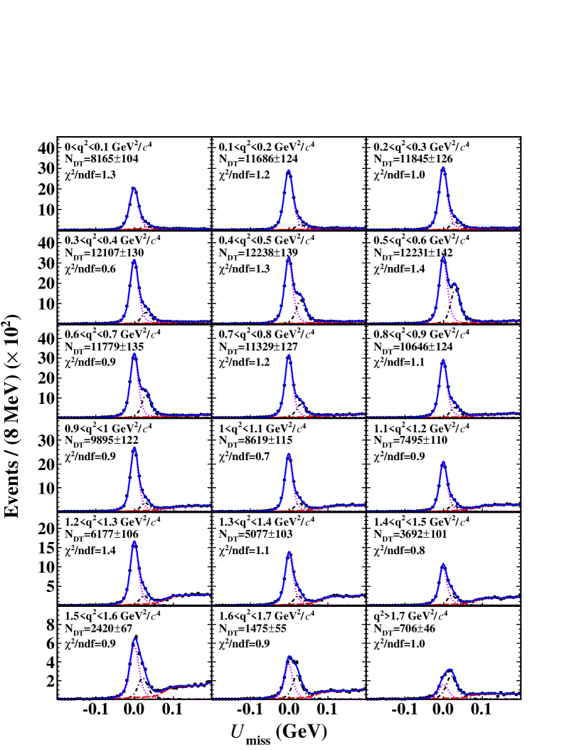
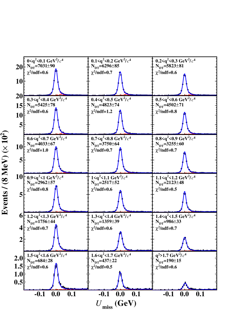
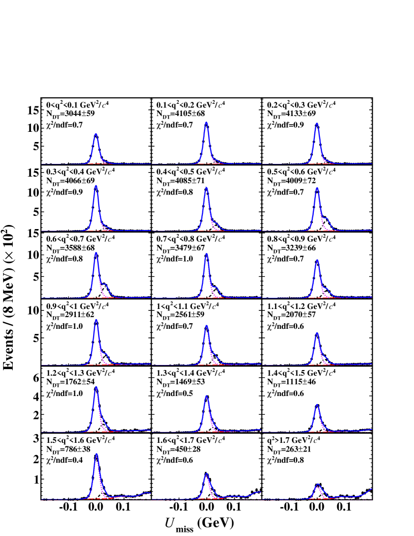
For each signal decay, the signal yield observed in each reconstructed interval is obtained from a fit to the distribution. The fitting method is the same as mentioned in Section VI.1. Figure 3 shows the results of the fits to the distributions in reconstructed intervals for semileptonic decays. Similar figures for , , and decays are available in Figs. 79 in Appendix.
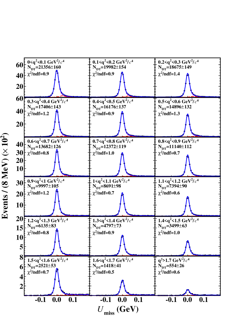
Table 6 lists the ranges, the fitted numbers of observed DT events (), the numbers of produced events () calculated by the weighted efficiency matrix and the decay rates () of semileptonic decays in individual intervals. Similar tables for , , and decays are available in Tables 1315 in Appendix.
VII.3 Construction of and statistical covariance matrices
To determine the hadronic transition form factor and , a least method is used to fit the partial decay rates of the different signal decays. Considering the correlations of the measured partial decay rates () among different intervals, the is given by
| (17) |
where is the theoretically expected decay rate in the -th interval, is the element of the inverse covariance matrix of the measured partial decay rates and is given by . Here, and are elements of the statistical and systematic covariance matrices, respectively. The elements of the statistical covariance matrix are defined as
| (18) |
where is the statistical uncertainty of the signal yield observed in the -th interval. The elements of the statistical covariance density matrices of , , and decays are presented in Tables 1619 in Appendix.
VII.4 Systematic uncertainties on partial decay rates
The sources of systematic uncertainties are discussed below.
ST yields
The systematic uncertainties associated with the number of tags are fully correlated across intervals. The element of the related systematic covariance matrix is calculated by
| (19) |
where is the relative uncertainty on the number of tags.
lifetime
The systematic uncertainties associated with the lifetime are fully correlated across the intervals. The element of the related systematic covariance matrix is calculated by
| (20) |
where and is the uncertainty on the lifetime pdg2022 .
MC statistics
The elements of the covariance matrix which accounts for the systematic uncertainties and correlations between the intervals are calculated by
| (21) |
where is the signal yield observed in the interval , and the covariances of the inverse efficiency matrix elements are given by
| (22) |
MC model
To estimate the uncertainty from the MC model, we vary the parameters of the two-parameter series expansion model by . The difference between the alternative and nominal efficiencies is taken as the systematic uncertainty for each signal decay. The element of the covariance matrix is defined as
| (23) |
where denotes the change of the partial decay rate in the -th interval.
Tracking, PID
The systematic uncertainties associated with the or tracking and PID efficiencies, and tracking and PID efficiencies are estimated by varying the corresponding correction factors for efficiencies within . Using the new efficiency matrix, the element of the corresponding systematic covariance matrix is calculated by
| (24) |
where denotes the change of the partial decay rate in the -th interval.
fit
The systematic covariance matrix arising from the uncertainty in the fit has elements
| (25) |
where is the systematic uncertainty of the signal yield observed in the interval obtained by varying the background shape in the fit as described in Section VI.2.
Remaining uncertainties
The remaining systematic uncertainties, include the and requirements, reconstruction, and quoted branching fractions, are assumed to be fully correlated across intervals, and the element of the corresponding systematic covariance matrix is calculated by
| (26) |
where . The systematic uncertainties on semileptonic decays in different intervals are shown in Table 7, and those of , , and decays are available in Tables 2022 in Appendix, as well as the elements of the systematic covariance density matrices for all signal decays.
| -th bin | 1 | 2 | 3 | 4 | 5 | 6 | 7 | 8 | 9 | 10 | 11 | 12 | 13 | 14 | 15 | 16 | 17 | 18 |
|---|---|---|---|---|---|---|---|---|---|---|---|---|---|---|---|---|---|---|
| 0.30 | 0.30 | 0.30 | 0.30 | 0.30 | 0.30 | 0.30 | 0.30 | 0.30 | 0.30 | 0.30 | 0.30 | 0.30 | 0.30 | 0.30 | 0.30 | 0.30 | 0.30 | |
| lifetime | 0.24 | 0.24 | 0.24 | 0.24 | 0.24 | 0.24 | 0.24 | 0.24 | 0.24 | 0.24 | 0.24 | 0.24 | 0.24 | 0.24 | 0.24 | 0.24 | 0.24 | 0.24 |
| MC statistics | 0.14 | 0.15 | 0.15 | 0.16 | 0.17 | 0.17 | 0.18 | 0.19 | 0.20 | 0.21 | 0.23 | 0.25 | 0.28 | 0.31 | 0.36 | 0.45 | 0.60 | 0.99 |
| MC model | 0.21 | 0.19 | 0.56 | 0.28 | 0.06 | 0.46 | 1.50 | 0.25 | 1.58 | 0.31 | 0.44 | 0.04 | 0.57 | 1.33 | 0.31 | 0.29 | 3.63 | 1.04 |
| tracking | 0.10 | 0.10 | 0.10 | 0.10 | 0.10 | 0.10 | 0.10 | 0.10 | 0.10 | 0.10 | 0.10 | 0.11 | 0.11 | 0.13 | 0.13 | 0.18 | 0.23 | 0.43 |
| PID | 0.10 | 0.10 | 0.10 | 0.10 | 0.10 | 0.10 | 0.10 | 0.10 | 0.10 | 0.10 | 0.10 | 0.10 | 0.10 | 0.10 | 0.10 | 0.10 | 0.10 | 0.13 |
| tracking | 0.10 | 0.10 | 0.10 | 0.10 | 0.10 | 0.10 | 0.10 | 0.10 | 0.10 | 0.10 | 0.10 | 0.10 | 0.10 | 0.10 | 0.10 | 0.10 | 0.10 | 0.10 |
| PID | 0.10 | 0.10 | 0.10 | 0.10 | 0.10 | 0.10 | 0.10 | 0.10 | 0.10 | 0.10 | 0.10 | 0.10 | 0.10 | 0.10 | 0.10 | 0.10 | 0.10 | 0.10 |
| fit | 0.18 | 0.16 | 0.18 | 0.16 | 0.15 | 0.17 | 0.15 | 0.16 | 0.10 | 0.11 | 0.10 | 0.09 | 0.09 | 0.11 | 0.08 | 0.14 | 0.18 | 0.34 |
| and cut | 0.10 | 0.10 | 0.10 | 0.10 | 0.10 | 0.10 | 0.10 | 0.10 | 0.10 | 0.10 | 0.10 | 0.10 | 0.10 | 0.10 | 0.10 | 0.10 | 0.10 | 0.10 |
| Total | 0.54 | 0.53 | 0.75 | 0.57 | 0.50 | 0.68 | 1.58 | 0.57 | 1.65 | 0.59 | 0.67 | 0.52 | 0.78 | 1.44 | 0.66 | 0.73 | 3.71 | 1.60 |
VII.5 Results based on individual fits
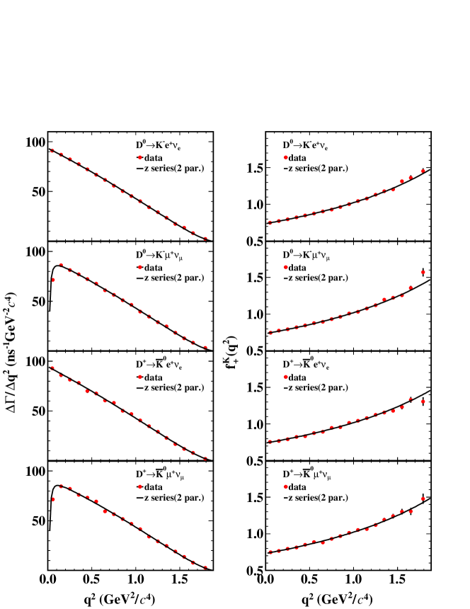
With the statistical and systematic covariance matrices described previously, we fit individually the partial decay rates of , , , and to obtain the fit parameters and from Eq. (9). The statistical uncertainties on the fit parameters are taken from the fit with the statistical covariance matrix, and the systematic uncertainties on the fit parameters are obtained by calculating the quadrature difference between the uncertainties of the fit parameters using the statistical covariance matrix and the uncertainties using the combined statistical and systematic covariance matrix.
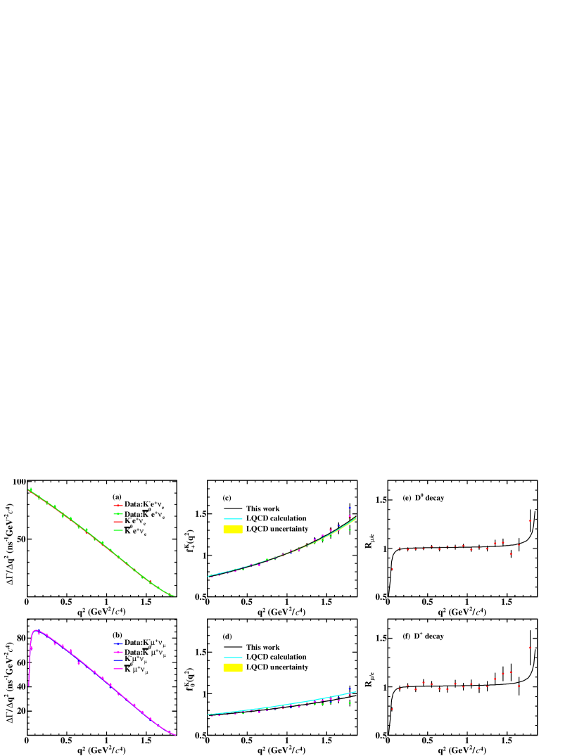
The sub-figures on the left of Fig. 4 show the individual fit results of , , , and . The sub-figures on the right of Fig. 4 show the projections of the form factor fits as a function of , where the points with error bars show the measured values of the form factor, which are obtained with
| (27) |
with
| (28) |
| (29) |
where and are the low and high boundaries of the -th bin. Both functions and are calculated using the two-parameter series expansion model.
The parameters obtained from the individual fits to the differential decay rates of , , , and are listed in Table 8.
| Case | Signal decay | ||||
|---|---|---|---|---|---|
| Individual fit | 0.48 | 16.3/16 | |||
| 0.62 | 17.1/16 | ||||
| 0.29 | 13.0/16 | ||||
| 0.45 | 10.6/16 | ||||
| Simultaneous fit | 0.44 | 60.9/70 |
VII.6 Results based on a simultaneous fit
To consider the correlation effects in the measurements of the hadronic form factor among the four signal decays, we perform a simultaneous fit to the partial decay rates of , , , and to obtain the product and .
In the simultaneous fit, the values of and are shared among the four signal decays. We still use the least method from Eq. (17) to obtain the fit parameters. The for these four semileptonic decay modes are combined into one vector with 72 components and the elements of the covariance matrix for the combined are redefined as , , where is the element of statistical covariance matrix, which is diagonal in blocks, i.e.
Here , , , and are the statistical covariance matrices obtained from each signal channel. The element of the correlated systematic covariance matrix is
| (30) |
The uncorrelated systematic covariance matrix is defined in blocks as
where , , , and are the uncorrelated systematic covariance matrices obtained from each signal channel.
Then, the elements of covariance density matrix for the simultaneous fit are available in Tables 2730 in Appendix.
With the modified and , we do the simultaneous fit to the partial decay rates of , which is shown in Fig. 5. The fitted parameters are and , which are summarized in Table 8.
VIII Summary
In summary, by analyzing 7.93 fb-1 of collision data collected at GeV with the BESIII detector, improved measurements of the semileptonic decays are performed. The absolute branching fractions of , , , and are determined to be , , and , respectively. Combining the branching fractions of semielectronic and semimuonic decays, we obtain the ratios of the two branching fractions and , which are consistent with the theoretical calculation Riggio:2017zwh . Our measurements support lepton flavor universality.
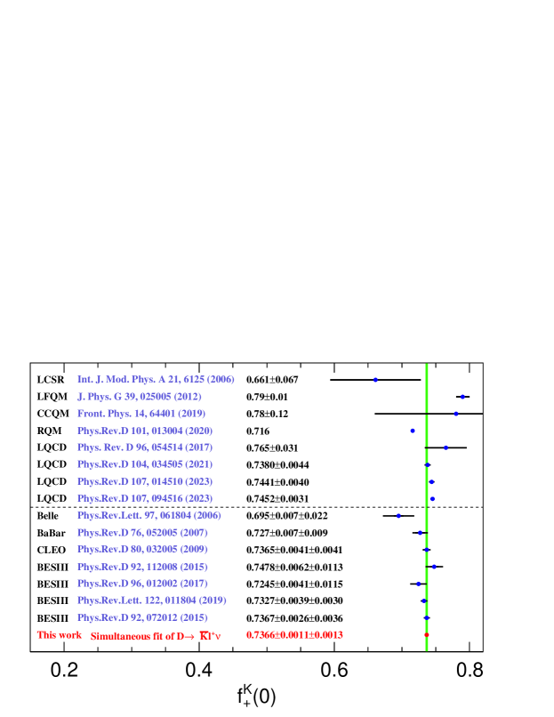
From the simultaneous fit to the partial decay rates of , , , and , the product of the hadronic form factor and the modulus of the CKM matrix element are determined to be . Taking the value of given by the PDG pdg2022 as input, we obtain the hadronic form factor . Conversely, using the calculated in LQCD FermilabLattice:2022gku , we obtain . The comparison of the value obtained in this work with the theoretical and experimental calculations is shown in Fig. 6. For the experimental calculations, the values of are updated by using the latest value of as mentioned before. The hadronic form factor measured in this work supersedes the previous BESIII results BESIII:2015tql ; BESIII:2018ccy ; BESIII:2017ylw ; BESIII:2015jmz , with the better precision. This is important to test different models and help to improve the precision of theoretical calculations.
Acknowledgements.
The BESIII Collaboration thanks the staff of BEPCII and the IHEP computing center for their strong support. This work is supported in part by National Key R&D Program of China under Contracts Nos. 2020YFA0406000, 2023YFA1606400, 2020YFA0406300; National Natural Science Foundation of China (NSFC) under Contracts Nos. 11635010, 11735014, 11935015, 11935016, 11935018, 12025502, 12035009, 12035013, 12061131003, 12192260, 12192261, 12192262, 12192263, 12192264, 12192265, 12221005, 12225509, 12235017, 12361141819; the Chinese Academy of Sciences (CAS) Large-Scale Scientific Facility Program; the CAS Center for Excellence in Particle Physics (CCEPP); Joint Large-Scale Scientific Facility Funds of the NSFC and CAS under Contract No. U1832207; 100 Talents Program of CAS; The Institute of Nuclear and Particle Physics (INPAC) and Shanghai Key Laboratory for Particle Physics and Cosmology; German Research Foundation DFG under Contracts Nos. 455635585, FOR5327, GRK 2149; Istituto Nazionale di Fisica Nucleare, Italy; Ministry of Development of Turkey under Contract No. DPT2006K-120470; National Research Foundation of Korea under Contract No. NRF-2022R1A2C1092335; National Science and Technology fund of Mongolia; National Science Research and Innovation Fund (NSRF) via the Program Management Unit for Human Resources & Institutional Development, Research and Innovation of Thailand under Contracts Nos. B16F640076, B50G670107; Polish National Science Centre under Contract No. 2019/35/O/ST2/02907; The Swedish Research Council; U. S. Department of Energy under Contract No. DE-FG02-05ER41374.References
- (1) V. Lubicz et al., Phys. Rev. D 96, 054514 (2017).
- (2) B. Chakraborty et al. (HPQCD Collaboration), Phys. Rev. D 104, 034505 (2021).
- (3) W. G. Parrott et al. (HPQCD collaboration), Phys. Rev. D 107, 014510 (2023).
- (4) A. Bazavov et al. (Fermilab Lattice and MILC Collaborations), Phys. Rev. D 107, 094516 (2023).
- (5) Y. L. Wu, M. Zhong and Y. B. Zuo, Int. J. Mod. Phys. A 21, 6125-6172 (2006).
- (6) R. C. Verma, J. Phys. G 39, 025005 (2012).
- (7) M. A. Ivanov, J. G. Körner, J. N. Pandya, P. Santorelli, N. R. Soni and C. T. Tran, Front. Phys. (Beijing) 14, 64401 (2019).
- (8) R. N. Faustov, V. O. Galkin and X. W. Kang, Phys. Rev. D 101, 013004 (2020).
- (9) B. C. Ke, J. Koponen, H. B. Li and Y. Zheng, Ann. Rev. Nucl. Part. Sci. 73, 285-314 (2023).
- (10) R. L. Workman et al. (Particle Data Group), Prog. Theor. Exp. Phys. 2022, 083C01 (2022).
- (11) M. Ablikim et al. (BES Collaboration), Phys. Lett. B 597, 39-46 (2004).
- (12) M. Ablikim et al. (BES Collaboration), Phys. Lett. B 608, 24-30 (2005).
- (13) M. Ablikim et al. (BES Collaboration), Phys. Lett. B 644, 20-24 (2007).
- (14) B. Aubert et al. (BaBar Collaboration), Phys. Rev. D 76, 052005 (2007).
- (15) L. Widhalm et al. (Belle Collaboration), Phys. Rev. Lett. 97, 061804 (2006).
- (16) G. S. Huang et al. (CLEO Collaboration), Phys. Rev. Lett. 95, 181801 (2005).
- (17) T. E. Coan et al. (CLEO Collaboration), Phys. Rev. Lett. 95, 181802 (2005).
- (18) S. Dobbs et al. (CLEO Collaboration), Phys. Rev. D 77, 112005 (2008).
- (19) D. Besson et al. (CLEO Collaboration), Phys. Rev. D 80, 032005 (2009).
- (20) M. Ablikim et al. (BESIII Collaboration), Phys. Rev. D 104, 052008 (2021).
- (21) M. Ablikim et al. (BESIII Collaboration), Phys. Rev. D 92, 072012 (2015).
- (22) M. Ablikim et al. (BESIII Collaboration), Phys. Rev. Lett. 122, 011804 (2019).
- (23) M. Ablikim et al. (BESIII Collaboration), Phys. Rev. D 92, 112008 (2015).
- (24) M. Ablikim et al. (BESIII Collaboration), Phys. Rev. D 96, 012002 (2017).
- (25) M. Ablikim et al. (BESIII Collaboration), Chin. Phys. C 40, 113001 (2016).
- (26) M. Ablikim et al. (BESIII Collaboration), Eur. Phys. J. C 76, 369 (2016).
- (27) M. Ablikim et al. (BESIII Collaboration), arXiv:2406.05827.
- (28) M. Ablikim et al. (BESIII Collaboration), Nucl. Instrum. Meth. A 614, 345 (2010).
- (29) C. H. Yu et al., Proceedings of IPAC2016, Busan, Korea, 2016, doi:10.18429/JACoW-IPAC2016-TUYA01.
- (30) M. Ablikim et al. (BESIII Collaboration), Chin. Phys. C 44, 040001 (2020).
- (31) H. B. Li and X. R. Lyu, Natl. Sci. Rev. 8, no.11, nwab181 (2021).
- (32) X. Li et al., Radiat. Detect. Technol. Methods 1, 13 (2017); Y. X. Guo et al., Radiat. Detect. Technol. Methods 1, 15 (2017); P. Cao et al., Nucl. Instrum. Meth. A 953, 163053 (2020).
- (33) S. Agostinelli et al. (GEANT4 Collaboration), Nucl. Instrum. Meth. A 506, 250 (2003).
- (34) K. X. Huang, Z. J. Li, Z. Qian, J. Zhu, H. Y. Li, Y. M. Zhang, S. S. Sun and Z. Y. You, Nucl. Sci. Tech. 33, 142 (2022).
- (35) S. Jadach, B. F. L. Ward and Z. Was, Phys. Rev. D 63, 113009 (2001); Comput. Phys. Commun. 130, 260 (2000).
- (36) T. Becher and R. J. Hill, Phys. Lett. B 633, 61 (2006).
- (37) D. J. Lange, Nucl. Instrum. Meth. A 462, 152 (2001); R. G. Ping, Chin. Phys. C 32, 599 (2008).
- (38) J. C. Chen, G. S. Huang, X. R. Qi, D. H. Zhang and Y. S. Zhu, Phys. Rev. D 62, 034003 (2000); R. L. Yang, R. G. Ping and H. Chen, Chin. Phys. Lett. 31, 061301 (2014).
- (39) E. Richter-Was, Phys. Lett. B 303, 163 (1993).
- (40) R. M. Baltrusaitis et al. (MARK III Collaboration), Phys. Rev. Lett. 56, 2140 (1986).
- (41) M. Ablikim et al. (BESIII Collaboration), Phys. Lett. B 734, 227 (2014).
- (42) K. Cranmer et al. (ROOT Collaboration), CERN-OPEN-2012-016.
- (43) H. Albrecht et al. (ARGUS Collaboration), Phys. Lett. B 241, 278 (1990).
- (44) C. G. Boyd, B. Grinstein and R. F. Lebed, Nucl. Phys. B 461, 493 (1996).
- (45) L. Riggio, G. Salerno and S. Simula, Eur. Phys. J. C 78, no.6, 501 (2018).
Appendix
Tables 9, 10, 11, and 12 report the elements of the weighted efficiency matrices for , , , and , respectively.
Figures 7, 8, and 9 show the results of the fits to the distributions in the reconstructed intervals for , , and , respectively.
Table 13, 14, and 15 list the ranges, the fitted numbers of observed DT events (), the numbers of produced events () calculated by the weighted efficiency matrix and the decay rates () of , , and in individual intervals.
Tables 16, 17, 18, and 19 report the elements of the statistical covariance density matrices for , , , and , respectively.
Tables 23, 24, 25 and 26 report the elements of the systematic covariance density matrices for , , , and , respectively.
Tables 27, 28, 29, and 30 report the elements of the covariance density matrix for the simultaneous fit.
| 1 | 2 | 3 | 4 | 5 | 6 | 7 | 8 | 9 | 10 | 11 | 12 | 13 | 14 | 15 | 16 | 17 | 18 | |
|---|---|---|---|---|---|---|---|---|---|---|---|---|---|---|---|---|---|---|
| 1 | 67.94 | 4.03 | 0.31 | 0.13 | 0.02 | 0.00 | 0.00 | 0.00 | 0.00 | 0.00 | 0.00 | 0.00 | 0.00 | 0.00 | 0.00 | 0.00 | 0.00 | 0.00 |
| 2 | 2.48 | 62.81 | 5.09 | 0.41 | 0.14 | 0.03 | 0.01 | 0.01 | 0.00 | 0.00 | 0.00 | 0.00 | 0.00 | 0.00 | 0.00 | 0.00 | 0.00 | 0.00 |
| 3 | 0.08 | 3.17 | 60.81 | 5.47 | 0.42 | 0.13 | 0.03 | 0.01 | 0.01 | 0.01 | 0.00 | 0.00 | 0.00 | 0.00 | 0.00 | 0.00 | 0.00 | 0.00 |
| 4 | 0.03 | 0.11 | 3.57 | 59.42 | 5.62 | 0.46 | 0.11 | 0.03 | 0.01 | 0.01 | 0.01 | 0.00 | 0.00 | 0.00 | 0.00 | 0.00 | 0.00 | 0.00 |
| 5 | 0.01 | 0.03 | 0.14 | 3.87 | 58.75 | 5.74 | 0.44 | 0.10 | 0.03 | 0.02 | 0.01 | 0.01 | 0.00 | 0.00 | 0.00 | 0.00 | 0.00 | 0.00 |
| 6 | 0.01 | 0.02 | 0.05 | 0.16 | 3.97 | 58.38 | 5.69 | 0.42 | 0.11 | 0.04 | 0.02 | 0.01 | 0.00 | 0.00 | 0.00 | 0.00 | 0.00 | 0.00 |
| 7 | 0.01 | 0.01 | 0.02 | 0.06 | 0.19 | 4.09 | 57.97 | 5.72 | 0.42 | 0.11 | 0.03 | 0.02 | 0.01 | 0.01 | 0.00 | 0.00 | 0.00 | 0.00 |
| 8 | 0.00 | 0.01 | 0.01 | 0.02 | 0.06 | 0.21 | 4.18 | 57.80 | 5.60 | 0.38 | 0.10 | 0.05 | 0.01 | 0.01 | 0.00 | 0.01 | 0.00 | 0.00 |
| 9 | 0.00 | 0.00 | 0.01 | 0.01 | 0.03 | 0.07 | 0.22 | 4.21 | 57.74 | 5.41 | 0.39 | 0.09 | 0.04 | 0.01 | 0.00 | 0.00 | 0.00 | 0.00 |
| 10 | 0.00 | 0.00 | 0.00 | 0.01 | 0.01 | 0.04 | 0.08 | 0.25 | 4.25 | 57.65 | 5.25 | 0.38 | 0.11 | 0.04 | 0.01 | 0.01 | 0.00 | 0.00 |
| 11 | 0.00 | 0.00 | 0.00 | 0.00 | 0.01 | 0.01 | 0.03 | 0.08 | 0.24 | 4.09 | 56.97 | 5.01 | 0.33 | 0.08 | 0.04 | 0.01 | 0.00 | 0.00 |
| 12 | 0.00 | 0.00 | 0.00 | 0.00 | 0.00 | 0.01 | 0.02 | 0.03 | 0.08 | 0.25 | 4.01 | 56.95 | 4.91 | 0.31 | 0.06 | 0.03 | 0.01 | 0.00 |
| 13 | 0.00 | 0.00 | 0.00 | 0.00 | 0.00 | 0.00 | 0.01 | 0.01 | 0.03 | 0.08 | 0.29 | 3.86 | 55.87 | 4.51 | 0.28 | 0.06 | 0.01 | 0.00 |
| 14 | 0.00 | 0.00 | 0.00 | 0.00 | 0.00 | 0.00 | 0.00 | 0.01 | 0.01 | 0.02 | 0.08 | 0.27 | 3.65 | 54.36 | 4.23 | 0.24 | 0.03 | 0.00 |
| 15 | 0.00 | 0.00 | 0.00 | 0.00 | 0.00 | 0.00 | 0.00 | 0.00 | 0.00 | 0.01 | 0.02 | 0.06 | 0.24 | 3.46 | 53.75 | 3.96 | 0.15 | 0.00 |
| 16 | 0.00 | 0.00 | 0.00 | 0.00 | 0.00 | 0.00 | 0.00 | 0.00 | 0.00 | 0.00 | 0.00 | 0.02 | 0.06 | 0.19 | 3.06 | 51.27 | 3.50 | 0.10 |
| 17 | 0.00 | 0.00 | 0.00 | 0.00 | 0.00 | 0.00 | 0.00 | 0.00 | 0.00 | 0.00 | 0.00 | 0.00 | 0.01 | 0.03 | 0.15 | 2.65 | 47.84 | 2.71 |
| 18 | 0.00 | 0.00 | 0.00 | 0.00 | 0.00 | 0.00 | 0.00 | 0.00 | 0.00 | 0.00 | 0.00 | 0.00 | 0.00 | 0.00 | 0.01 | 0.08 | 1.77 | 36.54 |
| 1 | 2 | 3 | 4 | 5 | 6 | 7 | 8 | 9 | 10 | 11 | 12 | 13 | 14 | 15 | 16 | 17 | 18 | |
|---|---|---|---|---|---|---|---|---|---|---|---|---|---|---|---|---|---|---|
| 1 | 38.04 | 1.14 | 0.02 | 0.00 | 0.00 | 0.00 | 0.00 | 0.00 | 0.00 | 0.00 | 0.00 | 0.00 | 0.00 | 0.00 | 0.00 | 0.00 | 0.00 | 0.00 |
| 2 | 1.52 | 38.87 | 1.79 | 0.03 | 0.01 | 0.00 | 0.00 | 0.00 | 0.00 | 0.00 | 0.00 | 0.00 | 0.00 | 0.00 | 0.00 | 0.00 | 0.00 | 0.00 |
| 3 | 0.04 | 1.71 | 40.76 | 2.28 | 0.05 | 0.01 | 0.00 | 0.00 | 0.00 | 0.00 | 0.00 | 0.00 | 0.00 | 0.00 | 0.00 | 0.00 | 0.00 | 0.00 |
| 4 | 0.01 | 0.05 | 2.17 | 43.37 | 2.71 | 0.08 | 0.02 | 0.01 | 0.00 | 0.00 | 0.00 | 0.00 | 0.00 | 0.00 | 0.00 | 0.00 | 0.00 | 0.00 |
| 5 | 0.01 | 0.02 | 0.08 | 2.61 | 46.18 | 3.14 | 0.13 | 0.03 | 0.02 | 0.01 | 0.00 | 0.00 | 0.00 | 0.00 | 0.00 | 0.00 | 0.00 | 0.00 |
| 6 | 0.01 | 0.01 | 0.03 | 0.10 | 2.99 | 49.00 | 3.46 | 0.15 | 0.05 | 0.02 | 0.01 | 0.00 | 0.00 | 0.00 | 0.00 | 0.00 | 0.00 | 0.00 |
| 7 | 0.00 | 0.01 | 0.02 | 0.03 | 0.14 | 3.33 | 51.75 | 3.70 | 0.18 | 0.06 | 0.03 | 0.01 | 0.00 | 0.00 | 0.00 | 0.00 | 0.00 | 0.00 |
| 8 | 0.00 | 0.00 | 0.01 | 0.02 | 0.06 | 0.18 | 3.65 | 53.83 | 3.88 | 0.21 | 0.06 | 0.02 | 0.01 | 0.01 | 0.00 | 0.00 | 0.00 | 0.00 |
| 9 | 0.00 | 0.00 | 0.00 | 0.01 | 0.02 | 0.05 | 0.18 | 3.80 | 55.97 | 3.93 | 0.23 | 0.08 | 0.04 | 0.02 | 0.00 | 0.00 | 0.00 | 0.00 |
| 10 | 0.00 | 0.00 | 0.00 | 0.01 | 0.01 | 0.03 | 0.07 | 0.23 | 3.85 | 57.24 | 3.97 | 0.27 | 0.08 | 0.03 | 0.01 | 0.01 | 0.00 | 0.00 |
| 11 | 0.00 | 0.00 | 0.00 | 0.00 | 0.01 | 0.02 | 0.03 | 0.07 | 0.24 | 3.97 | 58.22 | 3.82 | 0.23 | 0.07 | 0.03 | 0.01 | 0.00 | 0.00 |
| 12 | 0.00 | 0.00 | 0.00 | 0.00 | 0.01 | 0.01 | 0.01 | 0.03 | 0.07 | 0.25 | 3.90 | 58.46 | 3.73 | 0.23 | 0.08 | 0.02 | 0.00 | 0.00 |
| 13 | 0.00 | 0.00 | 0.00 | 0.00 | 0.00 | 0.00 | 0.01 | 0.01 | 0.03 | 0.08 | 0.28 | 3.76 | 57.18 | 3.58 | 0.20 | 0.05 | 0.01 | 0.00 |
| 14 | 0.00 | 0.00 | 0.00 | 0.00 | 0.00 | 0.00 | 0.00 | 0.00 | 0.01 | 0.02 | 0.07 | 0.28 | 3.47 | 56.01 | 3.29 | 0.17 | 0.03 | 0.01 |
| 15 | 0.00 | 0.00 | 0.00 | 0.00 | 0.00 | 0.00 | 0.00 | 0.00 | 0.00 | 0.01 | 0.02 | 0.06 | 0.25 | 3.26 | 54.77 | 3.09 | 0.12 | 0.02 |
| 16 | 0.00 | 0.00 | 0.00 | 0.00 | 0.00 | 0.00 | 0.00 | 0.00 | 0.00 | 0.00 | 0.01 | 0.01 | 0.05 | 0.19 | 2.95 | 52.16 | 2.87 | 0.05 |
| 17 | 0.00 | 0.00 | 0.00 | 0.00 | 0.00 | 0.00 | 0.00 | 0.00 | 0.00 | 0.00 | 0.00 | 0.00 | 0.01 | 0.03 | 0.14 | 2.42 | 48.84 | 2.01 |
| 18 | 0.00 | 0.00 | 0.00 | 0.00 | 0.00 | 0.00 | 0.00 | 0.00 | 0.00 | 0.00 | 0.00 | 0.00 | 0.00 | 0.00 | 0.02 | 0.07 | 1.70 | 37.02 |
| 1 | 2 | 3 | 4 | 5 | 6 | 7 | 8 | 9 | 10 | 11 | 12 | 13 | 14 | 15 | 16 | 17 | 18 | |
|---|---|---|---|---|---|---|---|---|---|---|---|---|---|---|---|---|---|---|
| 1 | 48.53 | 2.67 | 0.17 | 0.07 | 0.01 | 0.00 | 0.00 | 0.00 | 0.00 | 0.00 | 0.00 | 0.00 | 0.00 | 0.00 | 0.00 | 0.00 | 0.00 | 0.00 |
| 2 | 1.49 | 44.41 | 3.35 | 0.22 | 0.07 | 0.00 | 0.00 | 0.00 | 0.00 | 0.00 | 0.00 | 0.00 | 0.00 | 0.00 | 0.00 | 0.00 | 0.00 | 0.00 |
| 3 | 0.03 | 1.84 | 42.69 | 3.62 | 0.22 | 0.06 | 0.00 | 0.00 | 0.00 | 0.00 | 0.00 | 0.00 | 0.00 | 0.00 | 0.00 | 0.00 | 0.00 | 0.00 |
| 4 | 0.00 | 0.04 | 2.04 | 41.28 | 3.70 | 0.20 | 0.04 | 0.00 | 0.00 | 0.00 | 0.00 | 0.00 | 0.00 | 0.00 | 0.00 | 0.00 | 0.00 | 0.00 |
| 5 | 0.00 | 0.01 | 0.05 | 2.16 | 40.20 | 3.77 | 0.20 | 0.03 | 0.00 | 0.00 | 0.00 | 0.00 | 0.00 | 0.00 | 0.00 | 0.00 | 0.00 | 0.00 |
| 6 | 0.00 | 0.00 | 0.01 | 0.06 | 2.25 | 39.14 | 3.73 | 0.17 | 0.01 | 0.00 | 0.00 | 0.00 | 0.00 | 0.00 | 0.00 | 0.00 | 0.00 | 0.00 |
| 7 | 0.00 | 0.00 | 0.00 | 0.01 | 0.06 | 2.31 | 38.65 | 3.66 | 0.15 | 0.01 | 0.00 | 0.00 | 0.00 | 0.00 | 0.00 | 0.00 | 0.00 | 0.00 |
| 8 | 0.00 | 0.00 | 0.00 | 0.00 | 0.01 | 0.06 | 2.39 | 37.92 | 3.54 | 0.14 | 0.01 | 0.00 | 0.00 | 0.00 | 0.00 | 0.00 | 0.00 | 0.00 |
| 9 | 0.00 | 0.00 | 0.00 | 0.00 | 0.00 | 0.01 | 0.07 | 2.42 | 37.71 | 3.36 | 0.11 | 0.01 | 0.00 | 0.00 | 0.00 | 0.00 | 0.00 | 0.00 |
| 10 | 0.00 | 0.00 | 0.00 | 0.00 | 0.00 | 0.00 | 0.01 | 0.08 | 2.34 | 37.20 | 3.25 | 0.10 | 0.01 | 0.00 | 0.00 | 0.00 | 0.00 | 0.00 |
| 11 | 0.00 | 0.00 | 0.00 | 0.00 | 0.00 | 0.00 | 0.00 | 0.01 | 0.07 | 2.32 | 36.59 | 3.07 | 0.08 | 0.00 | 0.00 | 0.00 | 0.00 | 0.00 |
| 12 | 0.00 | 0.00 | 0.00 | 0.00 | 0.00 | 0.00 | 0.00 | 0.00 | 0.02 | 0.08 | 2.32 | 36.15 | 2.87 | 0.06 | 0.00 | 0.00 | 0.00 | 0.00 |
| 13 | 0.00 | 0.00 | 0.00 | 0.00 | 0.00 | 0.00 | 0.00 | 0.00 | 0.01 | 0.01 | 0.08 | 2.21 | 35.89 | 2.71 | 0.04 | 0.00 | 0.00 | 0.00 |
| 14 | 0.00 | 0.00 | 0.00 | 0.00 | 0.00 | 0.00 | 0.00 | 0.00 | 0.00 | 0.00 | 0.01 | 0.08 | 2.06 | 35.51 | 2.53 | 0.03 | 0.00 | 0.00 |
| 15 | 0.00 | 0.00 | 0.00 | 0.00 | 0.00 | 0.00 | 0.00 | 0.00 | 0.00 | 0.00 | 0.00 | 0.01 | 0.09 | 2.00 | 35.05 | 2.25 | 0.02 | 0.00 |
| 16 | 0.00 | 0.00 | 0.00 | 0.00 | 0.00 | 0.00 | 0.00 | 0.00 | 0.00 | 0.00 | 0.00 | 0.00 | 0.01 | 0.07 | 1.75 | 34.66 | 2.00 | 0.01 |
| 17 | 0.00 | 0.00 | 0.00 | 0.00 | 0.00 | 0.00 | 0.00 | 0.00 | 0.00 | 0.00 | 0.00 | 0.00 | 0.00 | 0.00 | 0.06 | 1.54 | 34.31 | 1.77 |
| 18 | 0.00 | 0.00 | 0.00 | 0.00 | 0.00 | 0.00 | 0.00 | 0.00 | 0.00 | 0.00 | 0.00 | 0.00 | 0.00 | 0.00 | 0.01 | 0.04 | 1.33 | 32.87 |
| 1 | 2 | 3 | 4 | 5 | 6 | 7 | 8 | 9 | 10 | 11 | 12 | 13 | 14 | 15 | 16 | 17 | 18 | |
|---|---|---|---|---|---|---|---|---|---|---|---|---|---|---|---|---|---|---|
| 1 | 31.24 | 0.90 | 0.00 | 0.00 | 0.00 | 0.00 | 0.00 | 0.00 | 0.00 | 0.00 | 0.00 | 0.00 | 0.00 | 0.00 | 0.00 | 0.00 | 0.01 | 0.01 |
| 2 | 1.05 | 30.73 | 1.36 | 0.01 | 0.00 | 0.00 | 0.00 | 0.00 | 0.00 | 0.00 | 0.00 | 0.00 | 0.00 | 0.00 | 0.01 | 0.01 | 0.01 | 0.00 |
| 3 | 0.02 | 1.12 | 31.34 | 1.67 | 0.01 | 0.00 | 0.00 | 0.00 | 0.00 | 0.00 | 0.00 | 0.00 | 0.00 | 0.00 | 0.00 | 0.00 | 0.01 | 0.01 |
| 4 | 0.00 | 0.02 | 1.42 | 32.64 | 2.01 | 0.03 | 0.00 | 0.00 | 0.00 | 0.00 | 0.00 | 0.00 | 0.00 | 0.00 | 0.00 | 0.00 | 0.00 | 0.01 |
| 5 | 0.00 | 0.00 | 0.02 | 1.62 | 33.99 | 2.16 | 0.02 | 0.00 | 0.00 | 0.00 | 0.00 | 0.00 | 0.00 | 0.00 | 0.00 | 0.00 | 0.00 | 0.00 |
| 6 | 0.00 | 0.00 | 0.00 | 0.03 | 1.86 | 35.12 | 2.31 | 0.02 | 0.00 | 0.00 | 0.00 | 0.00 | 0.00 | 0.00 | 0.00 | 0.01 | 0.02 | 0.01 |
| 7 | 0.00 | 0.00 | 0.00 | 0.00 | 0.04 | 2.01 | 36.06 | 2.44 | 0.04 | 0.00 | 0.00 | 0.01 | 0.00 | 0.00 | 0.01 | 0.01 | 0.03 | 0.02 |
| 8 | 0.00 | 0.00 | 0.00 | 0.00 | 0.01 | 0.04 | 2.19 | 36.89 | 2.50 | 0.03 | 0.01 | 0.00 | 0.00 | 0.01 | 0.01 | 0.01 | 0.01 | 0.01 |
| 9 | 0.00 | 0.00 | 0.00 | 0.00 | 0.01 | 0.01 | 0.05 | 2.28 | 37.36 | 2.52 | 0.04 | 0.01 | 0.00 | 0.00 | 0.00 | 0.01 | 0.01 | 0.00 |
| 10 | 0.00 | 0.00 | 0.00 | 0.00 | 0.00 | 0.00 | 0.01 | 0.07 | 2.24 | 37.14 | 2.44 | 0.02 | 0.01 | 0.01 | 0.01 | 0.01 | 0.00 | 0.00 |
| 11 | 0.00 | 0.00 | 0.00 | 0.00 | 0.00 | 0.01 | 0.01 | 0.02 | 0.06 | 2.26 | 37.01 | 2.34 | 0.03 | 0.01 | 0.00 | 0.01 | 0.01 | 0.00 |
| 12 | 0.00 | 0.00 | 0.00 | 0.00 | 0.00 | 0.00 | 0.00 | 0.01 | 0.02 | 0.07 | 2.21 | 36.36 | 2.11 | 0.03 | 0.01 | 0.01 | 0.00 | 0.00 |
| 13 | 0.00 | 0.00 | 0.00 | 0.00 | 0.01 | 0.01 | 0.00 | 0.01 | 0.00 | 0.01 | 0.07 | 2.12 | 36.27 | 2.08 | 0.02 | 0.01 | 0.00 | 0.00 |
| 14 | 0.00 | 0.00 | 0.00 | 0.00 | 0.01 | 0.00 | 0.00 | 0.01 | 0.01 | 0.01 | 0.01 | 0.08 | 2.04 | 36.00 | 1.91 | 0.01 | 0.00 | 0.00 |
| 15 | 0.00 | 0.01 | 0.00 | 0.00 | 0.00 | 0.00 | 0.01 | 0.01 | 0.01 | 0.01 | 0.02 | 0.02 | 0.06 | 1.93 | 35.32 | 1.78 | 0.01 | 0.00 |
| 16 | 0.00 | 0.00 | 0.00 | 0.00 | 0.01 | 0.00 | 0.01 | 0.01 | 0.00 | 0.01 | 0.01 | 0.01 | 0.01 | 0.05 | 1.69 | 34.99 | 1.61 | 0.00 |
| 17 | 0.00 | 0.01 | 0.00 | 0.00 | 0.01 | 0.01 | 0.01 | 0.01 | 0.01 | 0.00 | 0.00 | 0.00 | 0.00 | 0.01 | 0.05 | 1.56 | 34.29 | 1.28 |
| 18 | 0.01 | 0.01 | 0.01 | 0.01 | 0.01 | 0.01 | 0.00 | 0.00 | 0.00 | 0.00 | 0.00 | 0.00 | 0.00 | 0.00 | 0.01 | 0.03 | 1.13 | 32.84 |
| 1 | 2 | 3 | 4 | 5 | 6 | 7 | 8 | 9 | 10 | 11 | 12 | 13 | 14 | 15 | 16 | 17 | 18 | |
|---|---|---|---|---|---|---|---|---|---|---|---|---|---|---|---|---|---|---|
| 1 | 1.000 | -0.099 | 0.004 | -0.002 | 0.000 | 0.000 | 0.000 | 0.000 | 0.000 | 0.000 | 0.000 | 0.000 | 0.000 | 0.000 | 0.000 | 0.000 | 0.000 | 0.000 |
| 2 | -0.099 | 1.000 | -0.132 | 0.007 | -0.002 | 0.000 | 0.000 | 0.000 | 0.000 | 0.000 | 0.000 | 0.000 | 0.000 | 0.000 | 0.000 | 0.000 | 0.000 | 0.000 |
| 3 | 0.004 | -0.132 | 1.000 | -0.148 | 0.009 | -0.003 | 0.000 | 0.000 | 0.000 | 0.000 | 0.000 | 0.000 | 0.000 | 0.000 | 0.000 | 0.000 | 0.000 | 0.000 |
| 4 | -0.002 | 0.007 | -0.148 | 1.000 | -0.158 | 0.010 | -0.002 | 0.000 | 0.000 | 0.000 | 0.000 | 0.000 | 0.000 | 0.000 | 0.000 | 0.000 | 0.000 | 0.000 |
| 5 | 0.000 | -0.002 | 0.009 | -0.158 | 1.000 | -0.162 | 0.011 | -0.002 | 0.000 | 0.000 | 0.000 | 0.000 | 0.000 | 0.000 | 0.000 | 0.000 | 0.000 | 0.000 |
| 6 | 0.000 | 0.000 | -0.003 | 0.010 | -0.162 | 1.000 | -0.165 | 0.011 | -0.003 | -0.001 | 0.000 | 0.000 | 0.000 | 0.000 | 0.000 | 0.000 | 0.000 | 0.000 |
| 7 | 0.000 | 0.000 | 0.000 | -0.002 | 0.011 | -0.165 | 1.000 | -0.167 | 0.011 | -0.003 | 0.000 | 0.000 | 0.000 | 0.000 | 0.000 | 0.000 | 0.000 | 0.000 |
| 8 | 0.000 | 0.000 | 0.000 | 0.000 | -0.002 | 0.011 | -0.167 | 1.000 | -0.166 | 0.011 | -0.003 | -0.001 | 0.000 | 0.000 | 0.000 | 0.000 | 0.000 | 0.000 |
| 9 | 0.000 | 0.000 | 0.000 | 0.000 | 0.000 | -0.003 | 0.011 | -0.166 | 1.000 | -0.164 | 0.010 | -0.002 | -0.001 | 0.000 | 0.000 | 0.000 | 0.000 | 0.000 |
| 10 | 0.000 | 0.000 | 0.000 | 0.000 | 0.000 | -0.001 | -0.003 | 0.011 | -0.164 | 1.000 | -0.160 | 0.009 | -0.002 | 0.000 | 0.000 | 0.000 | 0.000 | 0.000 |
| 11 | 0.000 | 0.000 | 0.000 | 0.000 | 0.000 | 0.000 | 0.000 | -0.003 | 0.010 | -0.160 | 1.000 | -0.155 | 0.008 | -0.002 | -0.001 | 0.000 | 0.000 | 0.000 |
| 12 | 0.000 | 0.000 | 0.000 | 0.000 | 0.000 | 0.000 | 0.000 | -0.001 | -0.002 | 0.009 | -0.155 | 1.000 | -0.152 | 0.007 | -0.002 | -0.001 | 0.000 | 0.000 |
| 13 | 0.000 | 0.000 | 0.000 | 0.000 | 0.000 | 0.000 | 0.000 | 0.000 | -0.001 | -0.002 | 0.008 | -0.152 | 1.000 | -0.145 | 0.007 | -0.002 | 0.000 | 0.000 |
| 14 | 0.000 | 0.000 | 0.000 | 0.000 | 0.000 | 0.000 | 0.000 | 0.000 | 0.000 | 0.000 | -0.002 | 0.007 | -0.145 | 1.000 | -0.140 | 0.006 | -0.001 | 0.000 |
| 15 | 0.000 | 0.000 | 0.000 | 0.000 | 0.000 | 0.000 | 0.000 | 0.000 | 0.000 | 0.000 | -0.001 | -0.002 | 0.007 | -0.140 | 1.000 | -0.131 | 0.006 | 0.000 |
| 16 | 0.000 | 0.000 | 0.000 | 0.000 | 0.000 | 0.000 | 0.000 | 0.000 | 0.000 | 0.000 | 0.000 | -0.001 | -0.002 | 0.006 | -0.131 | 1.000 | -0.123 | 0.005 |
| 17 | 0.000 | 0.000 | 0.000 | 0.000 | 0.000 | 0.000 | 0.000 | 0.000 | 0.000 | 0.000 | 0.000 | 0.000 | 0.000 | -0.001 | 0.006 | -0.123 | 1.000 | -0.105 |
| 18 | 0.000 | 0.000 | 0.000 | 0.000 | 0.000 | 0.000 | 0.000 | 0.000 | 0.000 | 0.000 | 0.000 | 0.000 | 0.000 | 0.000 | 0.000 | 0.005 | -0.105 | 1.000 |
| 1 | 2 | 3 | 4 | 5 | 6 | 7 | 8 | 9 | 10 | 11 | 12 | 13 | 14 | 15 | 16 | 17 | 18 | |
|---|---|---|---|---|---|---|---|---|---|---|---|---|---|---|---|---|---|---|
| 1 | 1.000 | -0.068 | 0.003 | 0.000 | 0.000 | 0.000 | 0.000 | 0.000 | 0.000 | 0.000 | 0.000 | 0.000 | 0.000 | 0.000 | 0.000 | 0.000 | 0.000 | 0.000 |
| 2 | -0.068 | 1.000 | -0.088 | 0.005 | -0.001 | 0.000 | 0.000 | 0.000 | 0.000 | 0.000 | 0.000 | 0.000 | 0.000 | 0.000 | 0.000 | 0.000 | 0.000 | 0.000 |
| 3 | 0.003 | -0.088 | 1.000 | -0.105 | 0.007 | -0.001 | 0.000 | 0.000 | 0.000 | 0.000 | 0.000 | 0.000 | 0.000 | 0.000 | 0.000 | 0.000 | 0.000 | 0.000 |
| 4 | 0.000 | 0.005 | -0.105 | 1.000 | -0.118 | 0.008 | -0.001 | 0.000 | 0.000 | 0.000 | 0.000 | 0.000 | 0.000 | 0.000 | 0.000 | 0.000 | 0.000 | 0.000 |
| 5 | 0.000 | -0.001 | 0.007 | -0.118 | 1.000 | -0.128 | 0.008 | -0.002 | 0.000 | 0.000 | 0.000 | 0.000 | 0.000 | 0.000 | 0.000 | 0.000 | 0.000 | 0.000 |
| 6 | 0.000 | 0.000 | -0.001 | 0.008 | -0.128 | 1.000 | -0.134 | 0.008 | -0.002 | -0.001 | 0.000 | 0.000 | 0.000 | 0.000 | 0.000 | 0.000 | 0.000 | 0.000 |
| 7 | 0.000 | 0.000 | 0.000 | -0.001 | 0.008 | -0.134 | 1.000 | -0.138 | 0.008 | -0.002 | -0.001 | 0.000 | 0.000 | 0.000 | 0.000 | 0.000 | 0.000 | 0.000 |
| 8 | 0.000 | 0.000 | 0.000 | 0.000 | -0.002 | 0.008 | -0.138 | 1.000 | -0.138 | 0.007 | -0.002 | 0.000 | 0.000 | 0.000 | 0.000 | 0.000 | 0.000 | 0.000 |
| 9 | 0.000 | 0.000 | 0.000 | 0.000 | 0.000 | -0.002 | 0.008 | -0.138 | 1.000 | -0.136 | 0.006 | -0.002 | -0.001 | 0.000 | 0.000 | 0.000 | 0.000 | 0.000 |
| 10 | 0.000 | 0.000 | 0.000 | 0.000 | 0.000 | -0.001 | -0.002 | 0.007 | -0.136 | 1.000 | -0.136 | 0.005 | -0.002 | 0.000 | 0.000 | 0.000 | 0.000 | 0.000 |
| 11 | 0.000 | 0.000 | 0.000 | 0.000 | 0.000 | 0.000 | -0.001 | -0.002 | 0.006 | -0.136 | 1.000 | -0.131 | 0.004 | -0.002 | 0.000 | 0.000 | 0.000 | 0.000 |
| 12 | 0.000 | 0.000 | 0.000 | 0.000 | 0.000 | 0.000 | 0.000 | 0.000 | -0.002 | 0.005 | -0.131 | 1.000 | -0.128 | 0.003 | -0.002 | 0.000 | 0.000 | 0.000 |
| 13 | 0.000 | 0.000 | 0.000 | 0.000 | 0.000 | 0.000 | 0.000 | 0.000 | -0.001 | -0.002 | 0.004 | -0.128 | 1.000 | -0.123 | 0.003 | -0.001 | 0.000 | 0.000 |
| 14 | 0.000 | 0.000 | 0.000 | 0.000 | 0.000 | 0.000 | 0.000 | 0.000 | 0.000 | 0.000 | -0.002 | 0.003 | -0.123 | 1.000 | -0.117 | 0.005 | -0.001 | 0.000 |
| 15 | 0.000 | 0.000 | 0.000 | 0.000 | 0.000 | 0.000 | 0.000 | 0.000 | 0.000 | 0.000 | 0.000 | -0.002 | 0.003 | -0.117 | 1.000 | -0.119 | 0.003 | -0.001 |
| 16 | 0.000 | 0.000 | 0.000 | 0.000 | 0.000 | 0.000 | 0.000 | 0.000 | 0.000 | 0.000 | 0.000 | 0.000 | -0.001 | 0.005 | -0.119 | 1.000 | -0.104 | 0.004 |
| 17 | 0.000 | 0.000 | 0.000 | 0.000 | 0.000 | 0.000 | 0.000 | 0.000 | 0.000 | 0.000 | 0.000 | 0.000 | 0.000 | -0.001 | 0.003 | -0.104 | 1.000 | -0.087 |
| 18 | 0.000 | 0.000 | 0.000 | 0.000 | 0.000 | 0.000 | 0.000 | 0.000 | 0.000 | 0.000 | 0.000 | 0.000 | 0.000 | 0.000 | -0.001 | 0.004 | -0.087 | 1.000 |
| 1 | 2 | 3 | 4 | 5 | 6 | 7 | 8 | 9 | 10 | 11 | 12 | 13 | 14 | 15 | 16 | 17 | 18 | |
|---|---|---|---|---|---|---|---|---|---|---|---|---|---|---|---|---|---|---|
| 1 | 1.000 | -0.089 | 0.004 | -0.001 | 0.000 | 0.000 | 0.000 | 0.000 | 0.000 | 0.000 | 0.000 | 0.000 | 0.000 | 0.000 | 0.000 | 0.000 | 0.000 | 0.000 |
| 2 | -0.089 | 1.000 | -0.117 | 0.006 | -0.002 | 0.000 | 0.000 | 0.000 | 0.000 | 0.000 | 0.000 | 0.000 | 0.000 | 0.000 | 0.000 | 0.000 | 0.000 | 0.000 |
| 3 | 0.004 | -0.117 | 1.000 | -0.133 | 0.009 | -0.002 | 0.000 | 0.000 | 0.000 | 0.000 | 0.000 | 0.000 | 0.000 | 0.000 | 0.000 | 0.000 | 0.000 | 0.000 |
| 4 | -0.001 | 0.006 | -0.133 | 1.000 | -0.141 | 0.010 | -0.001 | 0.000 | 0.000 | 0.000 | 0.000 | 0.000 | 0.000 | 0.000 | 0.000 | 0.000 | 0.000 | 0.000 |
| 5 | 0.000 | -0.002 | 0.009 | -0.141 | 1.000 | -0.149 | 0.012 | -0.001 | 0.000 | 0.000 | 0.000 | 0.000 | 0.000 | 0.000 | 0.000 | 0.000 | 0.000 | 0.000 |
| 6 | 0.000 | 0.000 | -0.002 | 0.010 | -0.149 | 1.000 | -0.152 | 0.013 | -0.001 | 0.000 | 0.000 | 0.000 | 0.000 | 0.000 | 0.000 | 0.000 | 0.000 | 0.000 |
| 7 | 0.000 | 0.000 | 0.000 | -0.001 | 0.012 | -0.152 | 1.000 | -0.156 | 0.013 | -0.001 | 0.000 | 0.000 | 0.000 | 0.000 | 0.000 | 0.000 | 0.000 | 0.000 |
| 8 | 0.000 | 0.000 | 0.000 | 0.000 | -0.001 | 0.013 | -0.156 | 1.000 | -0.155 | 0.012 | -0.001 | 0.000 | 0.000 | 0.000 | 0.000 | 0.000 | 0.000 | 0.000 |
| 9 | 0.000 | 0.000 | 0.000 | 0.000 | 0.000 | -0.001 | 0.013 | -0.155 | 1.000 | -0.150 | 0.013 | -0.001 | 0.000 | 0.000 | 0.000 | 0.000 | 0.000 | 0.000 |
| 10 | 0.000 | 0.000 | 0.000 | 0.000 | 0.000 | 0.000 | -0.001 | 0.012 | -0.150 | 1.000 | -0.148 | 0.012 | -0.001 | 0.000 | 0.000 | 0.000 | 0.000 | 0.000 |
| 11 | 0.000 | 0.000 | 0.000 | 0.000 | 0.000 | 0.000 | 0.000 | -0.001 | 0.013 | -0.148 | 1.000 | -0.146 | 0.011 | -0.001 | 0.000 | 0.000 | 0.000 | 0.000 |
| 12 | 0.000 | 0.000 | 0.000 | 0.000 | 0.000 | 0.000 | 0.000 | 0.000 | -0.001 | 0.012 | -0.146 | 1.000 | -0.139 | 0.010 | -0.001 | 0.000 | 0.000 | 0.000 |
| 13 | 0.000 | 0.000 | 0.000 | 0.000 | 0.000 | 0.000 | 0.000 | 0.000 | 0.000 | -0.001 | 0.011 | -0.139 | 1.000 | -0.132 | 0.009 | -0.001 | 0.000 | 0.000 |
| 14 | 0.000 | 0.000 | 0.000 | 0.000 | 0.000 | 0.000 | 0.000 | 0.000 | 0.000 | 0.000 | -0.001 | 0.010 | -0.132 | 1.000 | -0.127 | 0.008 | 0.000 | 0.000 |
| 15 | 0.000 | 0.000 | 0.000 | 0.000 | 0.000 | 0.000 | 0.000 | 0.000 | 0.000 | 0.000 | 0.000 | -0.001 | 0.009 | -0.127 | 1.000 | -0.113 | 0.006 | -0.001 |
| 16 | 0.000 | 0.000 | 0.000 | 0.000 | 0.000 | 0.000 | 0.000 | 0.000 | 0.000 | 0.000 | 0.000 | 0.000 | -0.001 | 0.008 | -0.113 | 1.000 | -0.102 | 0.005 |
| 17 | 0.000 | 0.000 | 0.000 | 0.000 | 0.000 | 0.000 | 0.000 | 0.000 | 0.000 | 0.000 | 0.000 | 0.000 | 0.000 | 0.000 | 0.006 | -0.102 | 1.000 | -0.093 |
| 18 | 0.000 | 0.000 | 0.000 | 0.000 | 0.000 | 0.000 | 0.000 | 0.000 | 0.000 | 0.000 | 0.000 | 0.000 | 0.000 | 0.000 | -0.001 | 0.005 | -0.093 | 1.000 |
| 1 | 2 | 3 | 4 | 5 | 6 | 7 | 8 | 9 | 10 | 11 | 12 | 13 | 14 | 15 | 16 | 17 | 18 | |
|---|---|---|---|---|---|---|---|---|---|---|---|---|---|---|---|---|---|---|
| 1 | 1.000 | -0.063 | 0.003 | 0.000 | 0.000 | 0.000 | 0.000 | 0.000 | 0.000 | 0.000 | 0.000 | 0.000 | 0.000 | 0.000 | 0.000 | 0.000 | 0.000 | -0.001 |
| 2 | -0.063 | 1.000 | -0.080 | 0.005 | 0.000 | 0.000 | 0.000 | 0.000 | 0.000 | 0.000 | 0.000 | 0.000 | 0.000 | 0.000 | -0.001 | 0.000 | -0.001 | -0.001 |
| 3 | 0.003 | -0.080 | 1.000 | -0.096 | 0.007 | 0.000 | 0.000 | 0.000 | 0.000 | 0.000 | 0.000 | 0.000 | 0.000 | 0.000 | 0.000 | 0.000 | 0.000 | -0.001 |
| 4 | 0.000 | 0.005 | -0.096 | 1.000 | -0.109 | 0.008 | 0.000 | 0.000 | 0.000 | 0.000 | 0.000 | 0.000 | 0.000 | 0.000 | 0.000 | 0.000 | 0.000 | -0.001 |
| 5 | 0.000 | 0.000 | 0.007 | -0.109 | 1.000 | -0.116 | 0.009 | -0.001 | 0.000 | 0.000 | 0.000 | 0.000 | 0.000 | 0.000 | 0.000 | -0.001 | -0.001 | -0.001 |
| 6 | 0.000 | 0.000 | 0.000 | 0.008 | -0.116 | 1.000 | -0.121 | 0.010 | -0.001 | 0.000 | 0.000 | 0.000 | 0.000 | 0.000 | 0.000 | 0.000 | -0.001 | -0.001 |
| 7 | 0.000 | 0.000 | 0.000 | 0.000 | 0.009 | -0.121 | 1.000 | -0.126 | 0.010 | -0.001 | 0.000 | 0.000 | 0.000 | 0.000 | -0.001 | 0.000 | -0.001 | 0.000 |
| 8 | 0.000 | 0.000 | 0.000 | 0.000 | -0.001 | 0.010 | -0.126 | 1.000 | -0.128 | 0.010 | -0.001 | 0.000 | 0.000 | 0.000 | 0.000 | -0.001 | -0.001 | 0.000 |
| 9 | 0.000 | 0.000 | 0.000 | 0.000 | 0.000 | -0.001 | 0.010 | -0.128 | 1.000 | -0.127 | 0.009 | -0.001 | 0.000 | 0.000 | 0.000 | 0.000 | -0.001 | 0.000 |
| 10 | 0.000 | 0.000 | 0.000 | 0.000 | 0.000 | 0.000 | -0.001 | 0.010 | -0.127 | 1.000 | -0.126 | 0.009 | -0.001 | 0.000 | 0.000 | -0.001 | 0.000 | 0.000 |
| 11 | 0.000 | 0.000 | 0.000 | 0.000 | 0.000 | 0.000 | 0.000 | -0.001 | 0.009 | -0.126 | 1.000 | -0.123 | 0.008 | -0.001 | 0.000 | 0.000 | 0.000 | 0.000 |
| 12 | 0.000 | 0.000 | 0.000 | 0.000 | 0.000 | 0.000 | 0.000 | 0.000 | -0.001 | 0.009 | -0.123 | 1.000 | -0.116 | 0.007 | -0.001 | 0.000 | 0.000 | 0.000 |
| 13 | 0.000 | 0.000 | 0.000 | 0.000 | 0.000 | 0.000 | 0.000 | 0.000 | 0.000 | -0.001 | 0.008 | -0.116 | 1.000 | -0.114 | 0.007 | -0.001 | 0.000 | 0.000 |
| 14 | 0.000 | 0.000 | 0.000 | 0.000 | 0.000 | 0.000 | 0.000 | 0.000 | 0.000 | 0.000 | -0.001 | 0.007 | -0.114 | 1.000 | -0.108 | 0.006 | -0.001 | 0.000 |
| 15 | 0.000 | -0.001 | 0.000 | 0.000 | 0.000 | 0.000 | -0.001 | 0.000 | 0.000 | 0.000 | 0.000 | -0.001 | 0.007 | -0.108 | 1.000 | -0.100 | 0.005 | -0.001 |
| 16 | 0.000 | 0.000 | 0.000 | 0.000 | -0.001 | 0.000 | 0.000 | -0.001 | 0.000 | -0.001 | 0.000 | 0.000 | -0.001 | 0.006 | -0.100 | 1.000 | -0.095 | 0.004 |
| 17 | 0.000 | -0.001 | 0.000 | 0.000 | -0.001 | -0.001 | -0.001 | -0.001 | -0.001 | 0.000 | 0.000 | 0.000 | 0.000 | -0.001 | 0.005 | -0.095 | 1.000 | -0.073 |
| 18 | -0.001 | -0.001 | -0.001 | -0.001 | -0.001 | -0.001 | 0.000 | 0.000 | 0.000 | 0.000 | 0.000 | 0.000 | 0.000 | 0.000 | -0.001 | 0.004 | -0.073 | 1.000 |
| -th bin | 1 | 2 | 3 | 4 | 5 | 6 | 7 | 8 | 9 | 10 | 11 | 12 | 13 | 14 | 15 | 16 | 17 | 18 |
|---|---|---|---|---|---|---|---|---|---|---|---|---|---|---|---|---|---|---|
| 0.30 | 0.30 | 0.30 | 0.30 | 0.30 | 0.30 | 0.30 | 0.30 | 0.30 | 0.30 | 0.30 | 0.30 | 0.30 | 0.30 | 0.30 | 0.30 | 0.30 | 0.30 | |
| lifetime | 0.24 | 0.24 | 0.24 | 0.24 | 0.24 | 0.24 | 0.24 | 0.24 | 0.24 | 0.24 | 0.24 | 0.24 | 0.24 | 0.24 | 0.24 | 0.24 | 0.24 | 0.24 |
| MC statistics | 0.25 | 0.21 | 0.20 | 0.20 | 0.20 | 0.20 | 0.20 | 0.20 | 0.21 | 0.21 | 0.23 | 0.24 | 0.27 | 0.31 | 0.36 | 0.44 | 0.58 | 0.93 |
| MC model | 0.18 | 0.21 | 0.71 | 0.44 | 0.20 | 0.23 | 0.28 | 0.06 | 0.19 | 0.20 | 0.16 | 0.74 | 1.03 | 0.87 | 0.21 | 0.74 | 1.02 | 1.06 |
| tracking | 0.10 | 0.10 | 0.10 | 0.10 | 0.10 | 0.10 | 0.10 | 0.10 | 0.10 | 0.10 | 0.10 | 0.11 | 0.11 | 0.13 | 0.14 | 0.18 | 0.23 | 0.43 |
| PID | 0.10 | 0.10 | 0.10 | 0.10 | 0.10 | 0.10 | 0.10 | 0.10 | 0.10 | 0.10 | 0.10 | 0.10 | 0.10 | 0.10 | 0.10 | 0.10 | 0.10 | 0.18 |
| tracking | 0.10 | 0.10 | 0.10 | 0.10 | 0.10 | 0.10 | 0.10 | 0.10 | 0.10 | 0.10 | 0.10 | 0.10 | 0.10 | 0.10 | 0.10 | 0.10 | 0.10 | 0.10 |
| PID | 0.20 | 0.20 | 0.19 | 0.18 | 0.18 | 0.17 | 0.17 | 0.17 | 0.16 | 0.17 | 0.17 | 0.18 | 0.18 | 0.19 | 0.19 | 0.20 | 0.22 | 0.23 |
| fit | 0.24 | 0.11 | 0.11 | 0.11 | 0.10 | 0.14 | 0.12 | 0.13 | 0.15 | 0.15 | 0.11 | 0.15 | 0.11 | 0.18 | 0.17 | 0.21 | 0.18 | 0.26 |
| and cut | 0.10 | 0.10 | 0.10 | 0.10 | 0.10 | 0.10 | 0.10 | 0.10 | 0.10 | 0.10 | 0.10 | 0.10 | 0.10 | 0.10 | 0.10 | 0.10 | 0.10 | 0.10 |
| Total | 0.62 | 0.57 | 0.88 | 0.68 | 0.55 | 0.57 | 0.59 | 0.53 | 0.56 | 0.57 | 0.56 | 0.92 | 1.17 | 1.06 | 0.66 | 1.02 | 1.30 | 1.58 |
| -th bin | 1 | 2 | 3 | 4 | 5 | 6 | 7 | 8 | 9 | 10 | 11 | 12 | 13 | 14 | 15 | 16 | 17 | 18 |
|---|---|---|---|---|---|---|---|---|---|---|---|---|---|---|---|---|---|---|
| 0.30 | 0.30 | 0.30 | 0.30 | 0.30 | 0.30 | 0.30 | 0.30 | 0.30 | 0.30 | 0.30 | 0.30 | 0.30 | 0.30 | 0.30 | 0.30 | 0.30 | 0.30 | |
| lifetime | 0.48 | 0.48 | 0.48 | 0.48 | 0.48 | 0.48 | 0.48 | 0.48 | 0.48 | 0.48 | 0.48 | 0.48 | 0.48 | 0.48 | 0.48 | 0.48 | 0.48 | 0.48 |
| MC statistics | 0.19 | 0.19 | 0.20 | 0.21 | 0.22 | 0.23 | 0.25 | 0.26 | 0.27 | 0.29 | 0.32 | 0.34 | 0.38 | 0.43 | 0.49 | 0.59 | 0.77 | 1.09 |
| MC model | 0.32 | 0.66 | 0.70 | 0.22 | 0.91 | 0.60 | 1.11 | 0.27 | 1.14 | 0.38 | 0.90 | 0.01 | 0.99 | 0.02 | 0.39 | 2.18 | 0.17 | 0.46 |
| tracking | 0.10 | 0.10 | 0.10 | 0.10 | 0.10 | 0.10 | 0.10 | 0.10 | 0.10 | 0.10 | 0.10 | 0.10 | 0.10 | 0.10 | 0.10 | 0.10 | 0.10 | 0.10 |
| PID | 0.10 | 0.10 | 0.10 | 0.10 | 0.10 | 0.10 | 0.10 | 0.10 | 0.10 | 0.10 | 0.10 | 0.10 | 0.10 | 0.10 | 0.10 | 0.10 | 0.10 | 0.10 |
| fit | 0.53 | 1.34 | 0.26 | 0.55 | 1.65 | 1.29 | 0.04 | 0.58 | 0.20 | 0.05 | 0.22 | 0.17 | 0.84 | 0.05 | 0.04 | 0.05 | 0.32 | 0.06 |
| and cut | 0.10 | 0.10 | 0.10 | 0.10 | 0.10 | 0.10 | 0.10 | 0.10 | 0.10 | 0.10 | 0.10 | 0.10 | 0.10 | 0.10 | 0.10 | 0.10 | 0.10 | 0.10 |
| reconstruction | 0.75 | 0.72 | 0.68 | 0.65 | 0.60 | 0.60 | 0.70 | 0.82 | 0.95 | 1.11 | 1.31 | 1.44 | 1.48 | 1.55 | 1.62 | 1.72 | 1.75 | 1.93 |
| Quoted branching fractions | 0.07 | 0.07 | 0.07 | 0.07 | 0.07 | 0.07 | 0.07 | 0.07 | 0.07 | 0.07 | 0.07 | 0.07 | 0.07 | 0.07 | 0.07 | 0.07 | 0.07 | 0.07 |
| Total | 1.16 | 1.77 | 1.19 | 1.08 | 2.08 | 1.67 | 1.46 | 1.23 | 1.64 | 1.35 | 1.74 | 1.60 | 2.09 | 1.71 | 1.84 | 2.90 | 2.03 | 2.34 |
| -th bin | 1 | 2 | 3 | 4 | 5 | 6 | 7 | 8 | 9 | 10 | 11 | 12 | 13 | 14 | 15 | 16 | 17 | 18 |
|---|---|---|---|---|---|---|---|---|---|---|---|---|---|---|---|---|---|---|
| 0.30 | 0.30 | 0.30 | 0.30 | 0.30 | 0.30 | 0.30 | 0.30 | 0.30 | 0.30 | 0.30 | 0.30 | 0.30 | 0.30 | 0.30 | 0.30 | 0.30 | 0.30 | |
| lifetime | 0.48 | 0.48 | 0.48 | 0.48 | 0.48 | 0.48 | 0.48 | 0.48 | 0.48 | 0.48 | 0.48 | 0.48 | 0.48 | 0.48 | 0.48 | 0.48 | 0.48 | 0.48 |
| MC statistics | 0.29 | 0.25 | 0.25 | 0.25 | 0.25 | 0.25 | 0.26 | 0.26 | 0.28 | 0.29 | 0.31 | 0.34 | 0.38 | 0.42 | 0.48 | 0.58 | 0.74 | 1.02 |
| MC model | 0.71 | 0.18 | 0.32 | 0.79 | 0.28 | 0.18 | 0.61 | 0.26 | 0.76 | 0.33 | 1.53 | 0.77 | 0.78 | 1.41 | 0.74 | 0.23 | 1.47 | 1.75 |
| tracking | 0.10 | 0.10 | 0.10 | 0.10 | 0.10 | 0.10 | 0.10 | 0.10 | 0.10 | 0.10 | 0.10 | 0.10 | 0.10 | 0.10 | 0.10 | 0.10 | 0.10 | 0.10 |
| PID | 0.17 | 0.17 | 0.17 | 0.17 | 0.16 | 0.16 | 0.16 | 0.16 | 0.16 | 0.16 | 0.17 | 0.17 | 0.18 | 0.19 | 0.18 | 0.19 | 0.22 | 0.25 |
| fit | 0.03 | 0.10 | 0.03 | 0.23 | 0.25 | 0.05 | 0.19 | 0.17 | 0.07 | 0.07 | 0.06 | 0.06 | 0.07 | 0.05 | 0.06 | 0.13 | 0.10 | 0.18 |
| and cut | 0.10 | 0.10 | 0.10 | 0.10 | 0.10 | 0.10 | 0.10 | 0.10 | 0.10 | 0.10 | 0.10 | 0.10 | 0.10 | 0.10 | 0.10 | 0.10 | 0.10 | 0.10 |
| reconstruction | 1.05 | 0.71 | 0.68 | 0.65 | 0.60 | 0.60 | 0.70 | 0.82 | 0.95 | 1.11 | 1.30 | 1.44 | 1.48 | 1.55 | 1.62 | 1.72 | 1.77 | 1.96 |
| Quoted branching fractions | 0.07 | 0.07 | 0.07 | 0.07 | 0.07 | 0.07 | 0.07 | 0.07 | 0.07 | 0.07 | 0.07 | 0.07 | 0.07 | 0.07 | 0.07 | 0.07 | 0.07 | 0.07 |
| Total | 1.44 | 0.99 | 1.00 | 1.24 | 0.97 | 0.91 | 1.16 | 1.10 | 1.39 | 1.34 | 2.12 | 1.78 | 1.82 | 2.22 | 1.95 | 1.93 | 2.50 | 2.90 |
| 1 | 2 | 3 | 4 | 5 | 6 | 7 | 8 | 9 | 10 | 11 | 12 | 13 | 14 | 15 | 16 | 17 | 18 | |
|---|---|---|---|---|---|---|---|---|---|---|---|---|---|---|---|---|---|---|
| 1 | 1.000 | 0.773 | 0.747 | 0.789 | 0.730 | 0.762 | 0.586 | 0.767 | 0.580 | 0.774 | 0.759 | 0.680 | 0.719 | 0.600 | 0.683 | 0.626 | 0.474 | 0.491 |
| 2 | 0.773 | 1.000 | 0.704 | 0.782 | 0.733 | 0.745 | 0.556 | 0.759 | 0.549 | 0.763 | 0.743 | 0.685 | 0.700 | 0.571 | 0.673 | 0.618 | 0.441 | 0.472 |
| 3 | 0.747 | 0.704 | 1.000 | 0.756 | 0.578 | 0.842 | 0.851 | 0.740 | 0.849 | 0.783 | 0.832 | 0.518 | 0.838 | 0.845 | 0.686 | 0.616 | 0.784 | 0.634 |
| 4 | 0.789 | 0.782 | 0.756 | 1.000 | 0.658 | 0.788 | 0.655 | 0.764 | 0.650 | 0.780 | 0.781 | 0.643 | 0.753 | 0.664 | 0.687 | 0.626 | 0.554 | 0.529 |
| 5 | 0.730 | 0.733 | 0.578 | 0.658 | 1.000 | 0.580 | 0.351 | 0.686 | 0.341 | 0.670 | 0.618 | 0.693 | 0.555 | 0.373 | 0.594 | 0.552 | 0.224 | 0.341 |
| 6 | 0.762 | 0.745 | 0.842 | 0.788 | 0.580 | 1.000 | 0.777 | 0.751 | 0.787 | 0.784 | 0.817 | 0.559 | 0.812 | 0.789 | 0.688 | 0.620 | 0.712 | 0.601 |
| 7 | 0.586 | 0.556 | 0.851 | 0.655 | 0.351 | 0.777 | 1.000 | 0.588 | 0.969 | 0.674 | 0.773 | 0.291 | 0.821 | 0.944 | 0.586 | 0.514 | 0.951 | 0.670 |
| 8 | 0.767 | 0.759 | 0.740 | 0.764 | 0.686 | 0.751 | 0.588 | 1.000 | 0.584 | 0.754 | 0.745 | 0.637 | 0.713 | 0.614 | 0.662 | 0.605 | 0.501 | 0.495 |
| 9 | 0.580 | 0.549 | 0.849 | 0.650 | 0.341 | 0.787 | 0.969 | 0.584 | 1.000 | 0.656 | 0.771 | 0.283 | 0.820 | 0.946 | 0.582 | 0.510 | 0.955 | 0.670 |
| 10 | 0.774 | 0.763 | 0.783 | 0.780 | 0.670 | 0.784 | 0.674 | 0.754 | 0.656 | 1.000 | 0.746 | 0.620 | 0.755 | 0.681 | 0.678 | 0.617 | 0.579 | 0.537 |
| 11 | 0.759 | 0.743 | 0.832 | 0.781 | 0.618 | 0.817 | 0.773 | 0.745 | 0.771 | 0.746 | 1.000 | 0.523 | 0.803 | 0.773 | 0.683 | 0.617 | 0.694 | 0.592 |
| 12 | 0.680 | 0.685 | 0.518 | 0.643 | 0.693 | 0.559 | 0.291 | 0.637 | 0.283 | 0.620 | 0.523 | 1.000 | 0.460 | 0.317 | 0.548 | 0.513 | 0.170 | 0.301 |
| 13 | 0.719 | 0.700 | 0.838 | 0.753 | 0.555 | 0.812 | 0.821 | 0.713 | 0.820 | 0.755 | 0.803 | 0.460 | 1.000 | 0.799 | 0.664 | 0.594 | 0.757 | 0.613 |
| 14 | 0.600 | 0.571 | 0.845 | 0.664 | 0.373 | 0.789 | 0.944 | 0.614 | 0.946 | 0.681 | 0.773 | 0.317 | 0.799 | 1.000 | 0.569 | 0.525 | 0.923 | 0.663 |
| 15 | 0.683 | 0.673 | 0.686 | 0.687 | 0.594 | 0.688 | 0.586 | 0.662 | 0.582 | 0.678 | 0.683 | 0.548 | 0.664 | 0.569 | 1.000 | 0.489 | 0.503 | 0.477 |
| 16 | 0.626 | 0.618 | 0.616 | 0.626 | 0.552 | 0.620 | 0.514 | 0.605 | 0.510 | 0.617 | 0.617 | 0.513 | 0.594 | 0.525 | 0.489 | 1.000 | 0.420 | 0.437 |
| 17 | 0.474 | 0.441 | 0.784 | 0.554 | 0.224 | 0.712 | 0.951 | 0.501 | 0.955 | 0.579 | 0.694 | 0.170 | 0.757 | 0.923 | 0.503 | 0.420 | 1.000 | 0.631 |
| 18 | 0.491 | 0.472 | 0.634 | 0.529 | 0.341 | 0.601 | 0.670 | 0.495 | 0.670 | 0.537 | 0.592 | 0.301 | 0.613 | 0.663 | 0.477 | 0.437 | 0.631 | 1.000 |
| 1 | 2 | 3 | 4 | 5 | 6 | 7 | 8 | 9 | 10 | 11 | 12 | 13 | 14 | 15 | 16 | 17 | 18 | |
|---|---|---|---|---|---|---|---|---|---|---|---|---|---|---|---|---|---|---|
| 1 | 1.000 | 0.717 | 0.637 | 0.702 | 0.731 | 0.716 | 0.717 | 0.679 | 0.697 | 0.695 | 0.697 | 0.611 | 0.555 | 0.573 | 0.614 | 0.561 | 0.512 | 0.456 |
| 2 | 0.717 | 1.000 | 0.718 | 0.790 | 0.804 | 0.790 | 0.796 | 0.735 | 0.766 | 0.765 | 0.763 | 0.701 | 0.646 | 0.662 | 0.676 | 0.643 | 0.593 | 0.527 |
| 3 | 0.637 | 0.718 | 1.000 | 0.853 | 0.714 | 0.729 | 0.770 | 0.536 | 0.673 | 0.685 | 0.652 | 0.894 | 0.904 | 0.881 | 0.606 | 0.807 | 0.809 | 0.703 |
| 4 | 0.702 | 0.790 | 0.853 | 1.000 | 0.759 | 0.783 | 0.808 | 0.644 | 0.739 | 0.745 | 0.725 | 0.838 | 0.820 | 0.813 | 0.658 | 0.761 | 0.740 | 0.648 |
| 5 | 0.731 | 0.804 | 0.714 | 0.759 | 1.000 | 0.759 | 0.792 | 0.737 | 0.764 | 0.762 | 0.762 | 0.686 | 0.629 | 0.646 | 0.673 | 0.629 | 0.578 | 0.514 |
| 6 | 0.716 | 0.790 | 0.729 | 0.783 | 0.759 | 1.000 | 0.754 | 0.714 | 0.749 | 0.749 | 0.745 | 0.702 | 0.652 | 0.665 | 0.661 | 0.643 | 0.597 | 0.530 |
| 7 | 0.717 | 0.796 | 0.770 | 0.808 | 0.792 | 0.754 | 1.000 | 0.668 | 0.754 | 0.753 | 0.746 | 0.743 | 0.701 | 0.709 | 0.665 | 0.678 | 0.638 | 0.565 |
| 8 | 0.679 | 0.735 | 0.536 | 0.644 | 0.737 | 0.714 | 0.668 | 1.000 | 0.670 | 0.701 | 0.713 | 0.511 | 0.432 | 0.464 | 0.617 | 0.474 | 0.406 | 0.369 |
| 9 | 0.697 | 0.766 | 0.673 | 0.739 | 0.764 | 0.749 | 0.754 | 0.670 | 1.000 | 0.690 | 0.730 | 0.647 | 0.591 | 0.609 | 0.642 | 0.594 | 0.544 | 0.486 |
| 10 | 0.695 | 0.765 | 0.685 | 0.745 | 0.762 | 0.749 | 0.753 | 0.701 | 0.690 | 1.000 | 0.687 | 0.660 | 0.605 | 0.621 | 0.640 | 0.604 | 0.556 | 0.494 |
| 11 | 0.697 | 0.763 | 0.652 | 0.725 | 0.762 | 0.745 | 0.746 | 0.713 | 0.730 | 0.687 | 1.000 | 0.602 | 0.567 | 0.586 | 0.639 | 0.576 | 0.522 | 0.467 |
| 12 | 0.611 | 0.701 | 0.894 | 0.838 | 0.686 | 0.702 | 0.743 | 0.511 | 0.647 | 0.660 | 0.602 | 1.000 | 0.869 | 0.860 | 0.583 | 0.786 | 0.790 | 0.687 |
| 13 | 0.555 | 0.646 | 0.904 | 0.820 | 0.629 | 0.652 | 0.701 | 0.432 | 0.591 | 0.605 | 0.567 | 0.869 | 1.000 | 0.865 | 0.537 | 0.794 | 0.812 | 0.702 |
| 14 | 0.573 | 0.662 | 0.881 | 0.813 | 0.646 | 0.665 | 0.709 | 0.464 | 0.609 | 0.621 | 0.586 | 0.860 | 0.865 | 1.000 | 0.521 | 0.777 | 0.786 | 0.684 |
| 15 | 0.614 | 0.676 | 0.606 | 0.658 | 0.673 | 0.661 | 0.665 | 0.617 | 0.642 | 0.640 | 0.639 | 0.583 | 0.537 | 0.521 | 1.000 | 0.498 | 0.498 | 0.447 |
| 16 | 0.561 | 0.643 | 0.807 | 0.761 | 0.629 | 0.643 | 0.678 | 0.474 | 0.594 | 0.604 | 0.576 | 0.786 | 0.794 | 0.777 | 0.498 | 1.000 | 0.688 | 0.632 |
| 17 | 0.512 | 0.593 | 0.809 | 0.740 | 0.578 | 0.597 | 0.638 | 0.406 | 0.544 | 0.556 | 0.522 | 0.790 | 0.812 | 0.786 | 0.498 | 0.688 | 1.000 | 0.614 |
| 18 | 0.456 | 0.527 | 0.703 | 0.648 | 0.514 | 0.530 | 0.565 | 0.369 | 0.486 | 0.494 | 0.467 | 0.687 | 0.702 | 0.684 | 0.447 | 0.632 | 0.614 | 1.000 |
| 1 | 2 | 3 | 4 | 5 | 6 | 7 | 8 | 9 | 10 | 11 | 12 | 13 | 14 | 15 | 16 | 17 | 18 | |
|---|---|---|---|---|---|---|---|---|---|---|---|---|---|---|---|---|---|---|
| 1 | 1.000 | 0.629 | 0.686 | 0.645 | 0.573 | 0.593 | 0.620 | 0.632 | 0.647 | 0.662 | 0.677 | 0.613 | 0.651 | 0.579 | 0.586 | 0.572 | 0.464 | 0.399 |
| 2 | 0.629 | 1.000 | 0.650 | 0.573 | 0.604 | 0.586 | 0.666 | 0.559 | 0.674 | 0.591 | 0.655 | 0.494 | 0.630 | 0.468 | 0.511 | 0.617 | 0.386 | 0.348 |
| 3 | 0.686 | 0.650 | 1.000 | 0.547 | 0.647 | 0.618 | 0.711 | 0.580 | 0.715 | 0.611 | 0.686 | 0.500 | 0.659 | 0.474 | 0.525 | 0.655 | 0.393 | 0.358 |
| 4 | 0.645 | 0.573 | 0.547 | 1.000 | 0.428 | 0.523 | 0.525 | 0.562 | 0.547 | 0.580 | 0.578 | 0.544 | 0.554 | 0.513 | 0.510 | 0.472 | 0.407 | 0.346 |
| 5 | 0.573 | 0.604 | 0.647 | 0.428 | 1.000 | 0.484 | 0.659 | 0.477 | 0.647 | 0.504 | 0.595 | 0.379 | 0.571 | 0.360 | 0.424 | 0.601 | 0.305 | 0.288 |
| 6 | 0.593 | 0.586 | 0.618 | 0.523 | 0.484 | 1.000 | 0.549 | 0.507 | 0.603 | 0.524 | 0.581 | 0.432 | 0.556 | 0.408 | 0.448 | 0.546 | 0.336 | 0.304 |
| 7 | 0.620 | 0.666 | 0.711 | 0.525 | 0.659 | 0.549 | 1.000 | 0.461 | 0.728 | 0.550 | 0.663 | 0.408 | 0.637 | 0.388 | 0.466 | 0.682 | 0.333 | 0.318 |
| 8 | 0.632 | 0.559 | 0.580 | 0.562 | 0.477 | 0.507 | 0.461 | 1.000 | 0.491 | 0.585 | 0.583 | 0.551 | 0.562 | 0.521 | 0.520 | 0.481 | 0.416 | 0.355 |
| 9 | 0.647 | 0.674 | 0.715 | 0.547 | 0.647 | 0.603 | 0.728 | 0.491 | 1.000 | 0.541 | 0.694 | 0.466 | 0.667 | 0.445 | 0.512 | 0.691 | 0.376 | 0.352 |
| 10 | 0.662 | 0.591 | 0.611 | 0.580 | 0.504 | 0.524 | 0.550 | 0.585 | 0.541 | 1.000 | 0.586 | 0.599 | 0.615 | 0.564 | 0.567 | 0.535 | 0.453 | 0.390 |
| 11 | 0.677 | 0.655 | 0.686 | 0.578 | 0.595 | 0.581 | 0.663 | 0.583 | 0.694 | 0.586 | 1.000 | 0.513 | 0.683 | 0.536 | 0.574 | 0.651 | 0.442 | 0.396 |
| 12 | 0.613 | 0.494 | 0.500 | 0.544 | 0.379 | 0.432 | 0.408 | 0.551 | 0.466 | 0.599 | 0.513 | 1.000 | 0.498 | 0.599 | 0.562 | 0.415 | 0.469 | 0.388 |
| 13 | 0.651 | 0.630 | 0.659 | 0.554 | 0.571 | 0.556 | 0.637 | 0.562 | 0.667 | 0.615 | 0.683 | 0.498 | 1.000 | 0.472 | 0.563 | 0.632 | 0.432 | 0.387 |
| 14 | 0.579 | 0.468 | 0.474 | 0.513 | 0.360 | 0.408 | 0.388 | 0.521 | 0.445 | 0.564 | 0.536 | 0.599 | 0.472 | 1.000 | 0.478 | 0.402 | 0.446 | 0.370 |
| 15 | 0.586 | 0.511 | 0.525 | 0.510 | 0.424 | 0.448 | 0.466 | 0.520 | 0.512 | 0.567 | 0.574 | 0.562 | 0.563 | 0.478 | 1.000 | 0.429 | 0.434 | 0.367 |
| 16 | 0.572 | 0.617 | 0.655 | 0.472 | 0.601 | 0.546 | 0.682 | 0.481 | 0.691 | 0.535 | 0.651 | 0.415 | 0.632 | 0.402 | 0.429 | 1.000 | 0.298 | 0.331 |
| 17 | 0.464 | 0.386 | 0.393 | 0.407 | 0.305 | 0.336 | 0.333 | 0.416 | 0.376 | 0.453 | 0.442 | 0.469 | 0.432 | 0.446 | 0.434 | 0.298 | 1.000 | 0.232 |
| 18 | 0.399 | 0.348 | 0.358 | 0.346 | 0.288 | 0.304 | 0.318 | 0.355 | 0.352 | 0.390 | 0.396 | 0.388 | 0.387 | 0.370 | 0.367 | 0.331 | 0.232 | 1.000 |
| 1 | 2 | 3 | 4 | 5 | 6 | 7 | 8 | 9 | 10 | 11 | 12 | 13 | 14 | 15 | 16 | 17 | 18 | |
|---|---|---|---|---|---|---|---|---|---|---|---|---|---|---|---|---|---|---|
| 1 | 1.000 | 0.587 | 0.633 | 0.674 | 0.590 | 0.560 | 0.656 | 0.620 | 0.699 | 0.653 | 0.729 | 0.705 | 0.691 | 0.703 | 0.640 | 0.539 | 0.583 | 0.532 |
| 2 | 0.587 | 1.000 | 0.557 | 0.546 | 0.561 | 0.554 | 0.557 | 0.585 | 0.578 | 0.599 | 0.539 | 0.591 | 0.579 | 0.538 | 0.541 | 0.501 | 0.448 | 0.401 |
| 3 | 0.633 | 0.557 | 1.000 | 0.553 | 0.569 | 0.550 | 0.586 | 0.583 | 0.608 | 0.597 | 0.592 | 0.608 | 0.595 | 0.578 | 0.552 | 0.487 | 0.478 | 0.431 |
| 4 | 0.674 | 0.546 | 0.553 | 1.000 | 0.511 | 0.516 | 0.638 | 0.554 | 0.664 | 0.568 | 0.713 | 0.632 | 0.617 | 0.665 | 0.561 | 0.435 | 0.543 | 0.499 |
| 5 | 0.590 | 0.561 | 0.569 | 0.511 | 1.000 | 0.472 | 0.556 | 0.551 | 0.568 | 0.559 | 0.546 | 0.564 | 0.551 | 0.532 | 0.511 | 0.452 | 0.439 | 0.395 |
| 6 | 0.560 | 0.554 | 0.550 | 0.516 | 0.472 | 1.000 | 0.470 | 0.545 | 0.535 | 0.548 | 0.498 | 0.539 | 0.527 | 0.493 | 0.491 | 0.450 | 0.408 | 0.365 |
| 7 | 0.656 | 0.557 | 0.586 | 0.638 | 0.556 | 0.470 | 1.000 | 0.511 | 0.643 | 0.577 | 0.665 | 0.622 | 0.608 | 0.631 | 0.558 | 0.456 | 0.518 | 0.474 |
| 8 | 0.620 | 0.585 | 0.583 | 0.554 | 0.551 | 0.545 | 0.511 | 1.000 | 0.543 | 0.605 | 0.566 | 0.606 | 0.594 | 0.562 | 0.555 | 0.505 | 0.468 | 0.422 |
| 9 | 0.699 | 0.578 | 0.608 | 0.664 | 0.568 | 0.535 | 0.643 | 0.543 | 1.000 | 0.575 | 0.717 | 0.674 | 0.660 | 0.683 | 0.609 | 0.501 | 0.564 | 0.517 |
| 10 | 0.653 | 0.599 | 0.597 | 0.568 | 0.559 | 0.548 | 0.577 | 0.605 | 0.575 | 1.000 | 0.569 | 0.652 | 0.637 | 0.604 | 0.598 | 0.546 | 0.506 | 0.456 |
| 11 | 0.729 | 0.539 | 0.592 | 0.713 | 0.546 | 0.498 | 0.665 | 0.566 | 0.717 | 0.569 | 1.000 | 0.670 | 0.687 | 0.750 | 0.626 | 0.480 | 0.617 | 0.571 |
| 12 | 0.705 | 0.591 | 0.608 | 0.632 | 0.564 | 0.539 | 0.622 | 0.606 | 0.674 | 0.652 | 0.670 | 1.000 | 0.649 | 0.687 | 0.638 | 0.552 | 0.571 | 0.522 |
| 13 | 0.691 | 0.579 | 0.595 | 0.617 | 0.551 | 0.527 | 0.608 | 0.594 | 0.660 | 0.637 | 0.687 | 0.649 | 1.000 | 0.636 | 0.630 | 0.543 | 0.560 | 0.511 |
| 14 | 0.703 | 0.538 | 0.578 | 0.665 | 0.532 | 0.493 | 0.631 | 0.562 | 0.683 | 0.604 | 0.750 | 0.687 | 0.636 | 1.000 | 0.582 | 0.498 | 0.590 | 0.544 |
| 15 | 0.640 | 0.541 | 0.552 | 0.561 | 0.511 | 0.491 | 0.558 | 0.555 | 0.609 | 0.598 | 0.626 | 0.638 | 0.630 | 0.582 | 1.000 | 0.470 | 0.520 | 0.472 |
| 16 | 0.539 | 0.501 | 0.487 | 0.435 | 0.452 | 0.450 | 0.456 | 0.505 | 0.501 | 0.546 | 0.480 | 0.552 | 0.543 | 0.498 | 0.470 | 1.000 | 0.372 | 0.380 |
| 17 | 0.583 | 0.448 | 0.478 | 0.543 | 0.439 | 0.408 | 0.518 | 0.468 | 0.564 | 0.506 | 0.617 | 0.571 | 0.560 | 0.590 | 0.520 | 0.372 | 1.000 | 0.411 |
| 18 | 0.532 | 0.401 | 0.431 | 0.499 | 0.395 | 0.365 | 0.474 | 0.422 | 0.517 | 0.456 | 0.571 | 0.522 | 0.511 | 0.544 | 0.472 | 0.380 | 0.411 | 1.000 |
| 1 | 2 | 3 | 4 | 5 | 6 | 7 | 8 | 9 | 10 | 11 | 12 | 13 | 14 | 15 | 16 | 17 | 18 | 19 | 20 | 21 | 22 | 23 | 24 | 25 | 26 | 27 | 28 | 29 | 30 | 31 | 32 | 33 | 34 | 35 | 36 | |
|---|---|---|---|---|---|---|---|---|---|---|---|---|---|---|---|---|---|---|---|---|---|---|---|---|---|---|---|---|---|---|---|---|---|---|---|---|
| 1 | 1.000 | 0.085 | 0.217 | 0.166 | 0.122 | 0.181 | 0.241 | 0.138 | 0.236 | 0.138 | 0.147 | 0.084 | 0.142 | 0.184 | 0.087 | 0.076 | 0.192 | 0.070 | 0.018 | 0.016 | 0.016 | 0.016 | 0.014 | 0.014 | 0.013 | 0.013 | 0.011 | 0.012 | 0.010 | 0.010 | 0.009 | 0.008 | 0.007 | 0.006 | 0.005 | 0.003 |
| 2 | 0.085 | 1.000 | 0.087 | 0.157 | 0.110 | 0.161 | 0.208 | 0.124 | 0.203 | 0.124 | 0.131 | 0.078 | 0.125 | 0.159 | 0.078 | 0.068 | 0.164 | 0.062 | 0.017 | 0.015 | 0.015 | 0.015 | 0.013 | 0.013 | 0.012 | 0.012 | 0.011 | 0.011 | 0.010 | 0.009 | 0.008 | 0.008 | 0.007 | 0.005 | 0.005 | 0.003 |
| 3 | 0.217 | 0.087 | 1.000 | 0.095 | 0.120 | 0.250 | 0.424 | 0.166 | 0.417 | 0.175 | 0.203 | 0.073 | 0.208 | 0.317 | 0.110 | 0.093 | 0.369 | 0.111 | 0.014 | 0.012 | 0.012 | 0.013 | 0.011 | 0.011 | 0.010 | 0.011 | 0.009 | 0.009 | 0.008 | 0.008 | 0.007 | 0.007 | 0.006 | 0.005 | 0.004 | 0.003 |
| 4 | 0.166 | 0.157 | 0.095 | 1.000 | -0.033 | 0.182 | 0.249 | 0.127 | 0.245 | 0.129 | 0.141 | 0.072 | 0.138 | 0.189 | 0.081 | 0.070 | 0.206 | 0.070 | 0.015 | 0.013 | 0.013 | 0.014 | 0.011 | 0.012 | 0.011 | 0.011 | 0.010 | 0.010 | 0.009 | 0.008 | 0.007 | 0.007 | 0.006 | 0.005 | 0.004 | 0.003 |
| 5 | 0.122 | 0.110 | 0.120 | -0.033 | 1.000 | -0.037 | 0.102 | 0.087 | 0.092 | 0.084 | 0.083 | 0.066 | 0.074 | 0.076 | 0.054 | 0.048 | 0.063 | 0.034 | 0.015 | 0.013 | 0.013 | 0.013 | 0.011 | 0.012 | 0.011 | 0.011 | 0.010 | 0.010 | 0.009 | 0.008 | 0.007 | 0.007 | 0.006 | 0.005 | 0.004 | 0.003 |
| 6 | 0.181 | 0.161 | 0.250 | 0.182 | -0.037 | 1.000 | 0.244 | 0.150 | 0.325 | 0.145 | 0.166 | 0.067 | 0.168 | 0.249 | 0.092 | 0.078 | 0.285 | 0.088 | 0.014 | 0.012 | 0.012 | 0.012 | 0.010 | 0.011 | 0.009 | 0.010 | 0.009 | 0.009 | 0.008 | 0.007 | 0.007 | 0.006 | 0.005 | 0.004 | 0.004 | 0.003 |
| 7 | 0.241 | 0.208 | 0.424 | 0.249 | 0.102 | 0.244 | 1.000 | 0.100 | 0.634 | 0.214 | 0.266 | 0.056 | 0.283 | 0.472 | 0.134 | 0.110 | 0.577 | 0.157 | 0.009 | 0.008 | 0.008 | 0.008 | 0.007 | 0.007 | 0.006 | 0.006 | 0.006 | 0.006 | 0.005 | 0.005 | 0.004 | 0.004 | 0.004 | 0.003 | 0.002 | 0.002 |
| 8 | 0.138 | 0.124 | 0.166 | 0.127 | 0.087 | 0.150 | 0.100 | 1.000 | 0.095 | 0.115 | 0.112 | 0.060 | 0.111 | 0.148 | 0.066 | 0.057 | 0.159 | 0.056 | 0.013 | 0.011 | 0.011 | 0.012 | 0.010 | 0.010 | 0.009 | 0.010 | 0.008 | 0.009 | 0.008 | 0.007 | 0.006 | 0.006 | 0.005 | 0.004 | 0.004 | 0.002 |
| 9 | 0.236 | 0.203 | 0.417 | 0.245 | 0.092 | 0.325 | 0.634 | 0.095 | 1.000 | 0.116 | 0.267 | 0.053 | 0.278 | 0.465 | 0.131 | 0.108 | 0.570 | 0.155 | 0.008 | 0.007 | 0.007 | 0.007 | 0.006 | 0.006 | 0.006 | 0.006 | 0.005 | 0.005 | 0.005 | 0.005 | 0.004 | 0.004 | 0.003 | 0.003 | 0.002 | 0.002 |
| 10 | 0.138 | 0.124 | 0.175 | 0.129 | 0.084 | 0.145 | 0.214 | 0.115 | 0.116 | 1.000 | -0.022 | 0.065 | 0.114 | 0.163 | 0.067 | 0.058 | 0.179 | 0.060 | 0.012 | 0.011 | 0.011 | 0.011 | 0.009 | 0.009 | 0.008 | 0.009 | 0.008 | 0.008 | 0.007 | 0.007 | 0.006 | 0.006 | 0.005 | 0.004 | 0.003 | 0.002 |
| 11 | 0.147 | 0.131 | 0.203 | 0.141 | 0.083 | 0.166 | 0.266 | 0.112 | 0.267 | -0.022 | 1.000 | -0.086 | 0.142 | 0.198 | 0.074 | 0.063 | 0.228 | 0.071 | 0.011 | 0.010 | 0.010 | 0.010 | 0.008 | 0.009 | 0.008 | 0.008 | 0.007 | 0.007 | 0.006 | 0.006 | 0.006 | 0.005 | 0.004 | 0.004 | 0.003 | 0.002 |
| 12 | 0.084 | 0.078 | 0.073 | 0.072 | 0.066 | 0.067 | 0.056 | 0.060 | 0.053 | 0.065 | -0.086 | 1.000 | -0.089 | 0.051 | 0.035 | 0.032 | 0.034 | 0.022 | 0.011 | 0.010 | 0.009 | 0.010 | 0.008 | 0.009 | 0.008 | 0.008 | 0.007 | 0.007 | 0.006 | 0.006 | 0.005 | 0.005 | 0.004 | 0.003 | 0.003 | 0.002 |
| 13 | 0.142 | 0.125 | 0.208 | 0.138 | 0.074 | 0.168 | 0.283 | 0.111 | 0.278 | 0.114 | 0.142 | -0.089 | 1.000 | 0.102 | 0.079 | 0.060 | 0.246 | 0.074 | 0.010 | 0.008 | 0.008 | 0.008 | 0.007 | 0.007 | 0.007 | 0.007 | 0.006 | 0.006 | 0.005 | 0.005 | 0.005 | 0.004 | 0.004 | 0.003 | 0.003 | 0.002 |
| 14 | 0.184 | 0.159 | 0.317 | 0.189 | 0.076 | 0.249 | 0.472 | 0.148 | 0.465 | 0.163 | 0.198 | 0.051 | 0.102 | 1.000 | -0.009 | 0.089 | 0.425 | 0.117 | 0.007 | 0.006 | 0.006 | 0.007 | 0.006 | 0.006 | 0.005 | 0.005 | 0.005 | 0.005 | 0.004 | 0.004 | 0.004 | 0.003 | 0.003 | 0.002 | 0.002 | 0.001 |
| 15 | 0.087 | 0.078 | 0.110 | 0.081 | 0.054 | 0.092 | 0.134 | 0.066 | 0.131 | 0.067 | 0.074 | 0.035 | 0.079 | -0.009 | 1.000 | -0.089 | 0.116 | 0.038 | 0.008 | 0.007 | 0.007 | 0.007 | 0.006 | 0.006 | 0.005 | 0.006 | 0.005 | 0.005 | 0.004 | 0.004 | 0.004 | 0.004 | 0.003 | 0.002 | 0.002 | 0.001 |
| 16 | 0.076 | 0.068 | 0.093 | 0.070 | 0.048 | 0.078 | 0.110 | 0.057 | 0.108 | 0.058 | 0.063 | 0.032 | 0.060 | 0.089 | -0.089 | 1.000 | 0.008 | 0.038 | 0.007 | 0.006 | 0.006 | 0.006 | 0.005 | 0.005 | 0.005 | 0.005 | 0.004 | 0.004 | 0.004 | 0.004 | 0.003 | 0.003 | 0.003 | 0.002 | 0.002 | 0.001 |
| 17 | 0.192 | 0.164 | 0.369 | 0.206 | 0.063 | 0.285 | 0.577 | 0.159 | 0.570 | 0.179 | 0.228 | 0.034 | 0.246 | 0.425 | 0.116 | 0.008 | 1.000 | 0.070 | 0.003 | 0.003 | 0.003 | 0.003 | 0.003 | 0.003 | 0.002 | 0.003 | 0.002 | 0.002 | 0.002 | 0.002 | 0.002 | 0.002 | 0.001 | 0.001 | 0.001 | 0.001 |
| 18 | 0.070 | 0.062 | 0.111 | 0.070 | 0.034 | 0.088 | 0.157 | 0.056 | 0.155 | 0.060 | 0.071 | 0.022 | 0.074 | 0.117 | 0.038 | 0.038 | 0.070 | 1.000 | 0.003 | 0.003 | 0.003 | 0.003 | 0.002 | 0.002 | 0.002 | 0.002 | 0.002 | 0.002 | 0.002 | 0.002 | 0.002 | 0.001 | 0.001 | 0.001 | 0.001 | 0.001 |
| 19 | 0.018 | 0.017 | 0.014 | 0.015 | 0.015 | 0.014 | 0.009 | 0.013 | 0.008 | 0.012 | 0.011 | 0.011 | 0.010 | 0.007 | 0.008 | 0.007 | 0.003 | 0.003 | 1.000 | 0.216 | 0.277 | 0.227 | 0.237 | 0.221 | 0.251 | 0.222 | 0.264 | 0.245 | 0.272 | 0.228 | 0.256 | 0.202 | 0.197 | 0.219 | 0.140 | 0.106 |
| 20 | 0.016 | 0.015 | 0.012 | 0.013 | 0.013 | 0.012 | 0.008 | 0.011 | 0.007 | 0.011 | 0.010 | 0.010 | 0.008 | 0.006 | 0.007 | 0.006 | 0.003 | 0.003 | 0.216 | 1.000 | 0.203 | 0.214 | 0.261 | 0.229 | 0.282 | 0.203 | 0.288 | 0.226 | 0.274 | 0.189 | 0.257 | 0.168 | 0.177 | 0.246 | 0.120 | 0.095 |
| 21 | 0.016 | 0.015 | 0.012 | 0.013 | 0.013 | 0.012 | 0.008 | 0.011 | 0.007 | 0.011 | 0.010 | 0.009 | 0.008 | 0.006 | 0.007 | 0.006 | 0.003 | 0.003 | 0.277 | 0.203 | 1.000 | 0.102 | 0.269 | 0.227 | 0.284 | 0.198 | 0.287 | 0.220 | 0.270 | 0.180 | 0.253 | 0.160 | 0.171 | 0.246 | 0.115 | 0.092 |
| 22 | 0.016 | 0.015 | 0.013 | 0.014 | 0.013 | 0.012 | 0.008 | 0.012 | 0.007 | 0.011 | 0.010 | 0.010 | 0.008 | 0.007 | 0.007 | 0.006 | 0.003 | 0.003 | 0.227 | 0.214 | 0.102 | 1.000 | 0.062 | 0.175 | 0.182 | 0.170 | 0.193 | 0.185 | 0.201 | 0.175 | 0.188 | 0.155 | 0.148 | 0.156 | 0.106 | 0.079 |
| 23 | 0.014 | 0.013 | 0.011 | 0.011 | 0.011 | 0.010 | 0.007 | 0.010 | 0.006 | 0.009 | 0.008 | 0.008 | 0.007 | 0.006 | 0.006 | 0.005 | 0.003 | 0.002 | 0.237 | 0.261 | 0.269 | 0.062 | 1.000 | 0.093 | 0.280 | 0.167 | 0.270 | 0.188 | 0.242 | 0.140 | 0.227 | 0.125 | 0.142 | 0.234 | 0.092 | 0.077 |
| 24 | 0.014 | 0.013 | 0.011 | 0.012 | 0.012 | 0.011 | 0.007 | 0.010 | 0.006 | 0.009 | 0.009 | 0.009 | 0.007 | 0.006 | 0.006 | 0.005 | 0.003 | 0.002 | 0.221 | 0.229 | 0.227 | 0.175 | 0.093 | 1.000 | 0.110 | 0.171 | 0.227 | 0.177 | 0.214 | 0.145 | 0.201 | 0.129 | 0.137 | 0.193 | 0.092 | 0.073 |
| 25 | 0.013 | 0.012 | 0.010 | 0.011 | 0.011 | 0.009 | 0.006 | 0.009 | 0.006 | 0.008 | 0.008 | 0.008 | 0.007 | 0.005 | 0.005 | 0.005 | 0.002 | 0.002 | 0.251 | 0.282 | 0.284 | 0.182 | 0.280 | 0.110 | 1.000 | 0.059 | 0.305 | 0.200 | 0.264 | 0.147 | 0.247 | 0.132 | 0.153 | 0.259 | 0.098 | 0.082 |
| 26 | 0.013 | 0.012 | 0.011 | 0.011 | 0.011 | 0.010 | 0.006 | 0.010 | 0.006 | 0.009 | 0.008 | 0.008 | 0.007 | 0.005 | 0.006 | 0.005 | 0.003 | 0.002 | 0.222 | 0.203 | 0.198 | 0.170 | 0.167 | 0.171 | 0.059 | 1.000 | 0.072 | 0.194 | 0.200 | 0.176 | 0.189 | 0.156 | 0.150 | 0.158 | 0.108 | 0.081 |
| 27 | 0.011 | 0.011 | 0.009 | 0.010 | 0.010 | 0.009 | 0.006 | 0.008 | 0.005 | 0.008 | 0.007 | 0.007 | 0.006 | 0.005 | 0.005 | 0.004 | 0.002 | 0.002 | 0.264 | 0.288 | 0.287 | 0.193 | 0.270 | 0.227 | 0.305 | 0.072 | 1.000 | 0.105 | 0.285 | 0.170 | 0.260 | 0.153 | 0.170 | 0.263 | 0.112 | 0.092 |
| 28 | 0.012 | 0.011 | 0.009 | 0.010 | 0.010 | 0.009 | 0.006 | 0.009 | 0.005 | 0.008 | 0.007 | 0.007 | 0.006 | 0.005 | 0.005 | 0.004 | 0.002 | 0.002 | 0.245 | 0.226 | 0.220 | 0.185 | 0.188 | 0.177 | 0.200 | 0.194 | 0.105 | 1.000 | 0.117 | 0.209 | 0.217 | 0.178 | 0.171 | 0.184 | 0.123 | 0.093 |
| 29 | 0.010 | 0.010 | 0.008 | 0.009 | 0.009 | 0.008 | 0.005 | 0.008 | 0.005 | 0.007 | 0.006 | 0.006 | 0.005 | 0.004 | 0.004 | 0.004 | 0.002 | 0.002 | 0.272 | 0.274 | 0.270 | 0.201 | 0.242 | 0.214 | 0.264 | 0.200 | 0.285 | 0.117 | 1.000 | 0.093 | 0.268 | 0.182 | 0.187 | 0.242 | 0.130 | 0.102 |
| 30 | 0.010 | 0.009 | 0.008 | 0.008 | 0.008 | 0.007 | 0.005 | 0.007 | 0.005 | 0.007 | 0.006 | 0.006 | 0.005 | 0.004 | 0.004 | 0.004 | 0.002 | 0.002 | 0.228 | 0.189 | 0.180 | 0.175 | 0.140 | 0.145 | 0.147 | 0.176 | 0.170 | 0.209 | 0.093 | 1.000 | 0.086 | 0.197 | 0.170 | 0.142 | 0.128 | 0.093 |
| 31 | 0.009 | 0.008 | 0.007 | 0.007 | 0.007 | 0.007 | 0.004 | 0.006 | 0.004 | 0.006 | 0.006 | 0.005 | 0.005 | 0.004 | 0.004 | 0.003 | 0.002 | 0.002 | 0.256 | 0.257 | 0.253 | 0.188 | 0.227 | 0.201 | 0.247 | 0.189 | 0.260 | 0.217 | 0.268 | 0.086 | 1.000 | 0.069 | 0.185 | 0.229 | 0.124 | 0.097 |
| 32 | 0.008 | 0.008 | 0.007 | 0.007 | 0.007 | 0.006 | 0.004 | 0.006 | 0.004 | 0.006 | 0.005 | 0.005 | 0.004 | 0.003 | 0.004 | 0.003 | 0.002 | 0.001 | 0.202 | 0.168 | 0.160 | 0.155 | 0.125 | 0.129 | 0.132 | 0.156 | 0.153 | 0.178 | 0.182 | 0.197 | 0.069 | 1.000 | 0.045 | 0.134 | 0.114 | 0.083 |
| 33 | 0.007 | 0.007 | 0.006 | 0.006 | 0.006 | 0.005 | 0.004 | 0.005 | 0.003 | 0.005 | 0.004 | 0.004 | 0.004 | 0.003 | 0.003 | 0.003 | 0.001 | 0.001 | 0.197 | 0.177 | 0.171 | 0.148 | 0.142 | 0.137 | 0.153 | 0.150 | 0.170 | 0.171 | 0.187 | 0.170 | 0.185 | 0.045 | 1.000 | 0.054 | 0.111 | 0.078 |
| 34 | 0.006 | 0.005 | 0.005 | 0.005 | 0.005 | 0.004 | 0.003 | 0.004 | 0.003 | 0.004 | 0.004 | 0.003 | 0.003 | 0.002 | 0.002 | 0.002 | 0.001 | 0.001 | 0.219 | 0.246 | 0.246 | 0.156 | 0.234 | 0.193 | 0.259 | 0.158 | 0.263 | 0.184 | 0.242 | 0.142 | 0.229 | 0.134 | 0.054 | 1.000 | 0.010 | 0.084 |
| 35 | 0.005 | 0.005 | 0.004 | 0.004 | 0.004 | 0.004 | 0.002 | 0.004 | 0.002 | 0.003 | 0.003 | 0.003 | 0.003 | 0.002 | 0.002 | 0.002 | 0.001 | 0.001 | 0.140 | 0.120 | 0.115 | 0.106 | 0.092 | 0.092 | 0.098 | 0.108 | 0.112 | 0.123 | 0.130 | 0.128 | 0.124 | 0.114 | 0.111 | 0.010 | 1.000 | -0.030 |
| 36 | 0.003 | 0.003 | 0.003 | 0.003 | 0.003 | 0.003 | 0.002 | 0.002 | 0.002 | 0.002 | 0.002 | 0.002 | 0.002 | 0.001 | 0.001 | 0.001 | 0.001 | 0.001 | 0.106 | 0.095 | 0.092 | 0.079 | 0.077 | 0.073 | 0.082 | 0.081 | 0.092 | 0.093 | 0.102 | 0.093 | 0.097 | 0.083 | 0.078 | 0.084 | -0.030 | 1.000 |
| 37 | 38 | 39 | 40 | 41 | 42 | 43 | 44 | 45 | 46 | 47 | 48 | 49 | 50 | 51 | 52 | 53 | 54 | 55 | 56 | 57 | 58 | 59 | 60 | 61 | 62 | 63 | 64 | 65 | 66 | 67 | 68 | 69 | 70 | 71 | 72 | |
|---|---|---|---|---|---|---|---|---|---|---|---|---|---|---|---|---|---|---|---|---|---|---|---|---|---|---|---|---|---|---|---|---|---|---|---|---|
| 1 | 0.069 | 0.064 | 0.054 | 0.058 | 0.057 | 0.051 | 0.033 | 0.050 | 0.031 | 0.046 | 0.043 | 0.042 | 0.037 | 0.029 | 0.030 | 0.027 | 0.015 | 0.016 | 0.004 | 0.003 | 0.003 | 0.003 | 0.003 | 0.003 | 0.003 | 0.003 | 0.002 | 0.003 | 0.002 | 0.002 | 0.002 | 0.002 | 0.002 | 0.001 | 0.001 | 0.001 |
| 2 | 0.079 | 0.074 | 0.062 | 0.067 | 0.066 | 0.059 | 0.038 | 0.057 | 0.036 | 0.053 | 0.049 | 0.048 | 0.042 | 0.033 | 0.034 | 0.032 | 0.017 | 0.019 | 0.005 | 0.004 | 0.004 | 0.004 | 0.003 | 0.003 | 0.003 | 0.003 | 0.003 | 0.003 | 0.003 | 0.002 | 0.002 | 0.002 | 0.002 | 0.001 | 0.001 | 0.001 |
| 3 | 0.068 | 0.064 | 0.054 | 0.058 | 0.057 | 0.051 | 0.033 | 0.050 | 0.031 | 0.046 | 0.043 | 0.042 | 0.037 | 0.029 | 0.030 | 0.027 | 0.015 | 0.016 | 0.004 | 0.003 | 0.003 | 0.003 | 0.003 | 0.003 | 0.003 | 0.003 | 0.002 | 0.003 | 0.002 | 0.002 | 0.002 | 0.002 | 0.002 | 0.001 | 0.001 | 0.001 |
| 4 | 0.072 | 0.068 | 0.057 | 0.061 | 0.061 | 0.054 | 0.035 | 0.053 | 0.033 | 0.049 | 0.045 | 0.044 | 0.039 | 0.031 | 0.032 | 0.029 | 0.016 | 0.017 | 0.004 | 0.004 | 0.004 | 0.004 | 0.003 | 0.003 | 0.003 | 0.003 | 0.003 | 0.003 | 0.002 | 0.002 | 0.002 | 0.002 | 0.002 | 0.001 | 0.001 | 0.001 |
| 5 | 0.071 | 0.067 | 0.056 | 0.060 | 0.060 | 0.053 | 0.035 | 0.052 | 0.033 | 0.048 | 0.044 | 0.044 | 0.038 | 0.030 | 0.031 | 0.029 | 0.015 | 0.017 | 0.004 | 0.004 | 0.003 | 0.004 | 0.003 | 0.003 | 0.003 | 0.003 | 0.003 | 0.003 | 0.002 | 0.002 | 0.002 | 0.002 | 0.002 | 0.001 | 0.001 | 0.001 |
| 6 | 0.069 | 0.065 | 0.054 | 0.058 | 0.058 | 0.052 | 0.033 | 0.050 | 0.032 | 0.046 | 0.043 | 0.042 | 0.037 | 0.029 | 0.030 | 0.028 | 0.015 | 0.016 | 0.004 | 0.003 | 0.003 | 0.003 | 0.003 | 0.003 | 0.003 | 0.003 | 0.002 | 0.003 | 0.002 | 0.002 | 0.002 | 0.002 | 0.002 | 0.001 | 0.001 | 0.001 |
| 7 | 0.069 | 0.064 | 0.054 | 0.058 | 0.058 | 0.051 | 0.033 | 0.050 | 0.032 | 0.046 | 0.043 | 0.042 | 0.037 | 0.029 | 0.030 | 0.028 | 0.015 | 0.016 | 0.004 | 0.003 | 0.003 | 0.003 | 0.003 | 0.003 | 0.003 | 0.003 | 0.002 | 0.003 | 0.002 | 0.002 | 0.002 | 0.002 | 0.002 | 0.001 | 0.001 | 0.001 |
| 8 | 0.071 | 0.067 | 0.056 | 0.060 | 0.060 | 0.053 | 0.035 | 0.052 | 0.033 | 0.048 | 0.044 | 0.044 | 0.038 | 0.030 | 0.031 | 0.029 | 0.015 | 0.017 | 0.004 | 0.004 | 0.003 | 0.004 | 0.003 | 0.003 | 0.003 | 0.003 | 0.003 | 0.003 | 0.002 | 0.002 | 0.002 | 0.002 | 0.002 | 0.001 | 0.001 | 0.001 |
| 9 | 0.068 | 0.064 | 0.054 | 0.058 | 0.057 | 0.051 | 0.033 | 0.050 | 0.031 | 0.046 | 0.043 | 0.042 | 0.036 | 0.029 | 0.030 | 0.027 | 0.015 | 0.016 | 0.004 | 0.003 | 0.003 | 0.003 | 0.003 | 0.003 | 0.003 | 0.003 | 0.002 | 0.003 | 0.002 | 0.002 | 0.002 | 0.002 | 0.002 | 0.001 | 0.001 | 0.001 |
| 10 | 0.065 | 0.061 | 0.051 | 0.055 | 0.054 | 0.049 | 0.032 | 0.047 | 0.030 | 0.044 | 0.041 | 0.040 | 0.035 | 0.027 | 0.028 | 0.026 | 0.014 | 0.015 | 0.004 | 0.003 | 0.003 | 0.003 | 0.003 | 0.003 | 0.003 | 0.003 | 0.002 | 0.002 | 0.002 | 0.002 | 0.002 | 0.002 | 0.001 | 0.001 | 0.001 | 0.001 |
| 11 | 0.061 | 0.057 | 0.048 | 0.051 | 0.051 | 0.045 | 0.029 | 0.044 | 0.028 | 0.041 | 0.038 | 0.037 | 0.032 | 0.026 | 0.026 | 0.024 | 0.013 | 0.014 | 0.003 | 0.003 | 0.003 | 0.003 | 0.003 | 0.003 | 0.002 | 0.003 | 0.002 | 0.002 | 0.002 | 0.002 | 0.002 | 0.002 | 0.001 | 0.001 | 0.001 | 0.001 |
| 12 | 0.052 | 0.049 | 0.041 | 0.044 | 0.044 | 0.039 | 0.025 | 0.038 | 0.024 | 0.035 | 0.032 | 0.032 | 0.028 | 0.022 | 0.023 | 0.021 | 0.011 | 0.013 | 0.003 | 0.003 | 0.003 | 0.003 | 0.002 | 0.002 | 0.002 | 0.002 | 0.002 | 0.002 | 0.002 | 0.002 | 0.001 | 0.001 | 0.001 | 0.001 | 0.001 | 0.001 |
| 13 | 0.044 | 0.041 | 0.034 | 0.037 | 0.036 | 0.033 | 0.021 | 0.032 | 0.020 | 0.029 | 0.027 | 0.027 | 0.023 | 0.018 | 0.019 | 0.018 | 0.010 | 0.011 | 0.002 | 0.002 | 0.002 | 0.002 | 0.002 | 0.002 | 0.002 | 0.002 | 0.002 | 0.002 | 0.001 | 0.001 | 0.001 | 0.001 | 0.001 | 0.001 | 0.001 | 0.000 |
| 14 | 0.040 | 0.038 | 0.032 | 0.034 | 0.034 | 0.030 | 0.020 | 0.029 | 0.019 | 0.027 | 0.025 | 0.025 | 0.022 | 0.017 | 0.018 | 0.017 | 0.009 | 0.010 | 0.002 | 0.002 | 0.002 | 0.002 | 0.002 | 0.002 | 0.002 | 0.002 | 0.001 | 0.001 | 0.001 | 0.001 | 0.001 | 0.001 | 0.001 | 0.001 | 0.001 | 0.000 |
| 15 | 0.032 | 0.030 | 0.026 | 0.027 | 0.027 | 0.024 | 0.016 | 0.024 | 0.015 | 0.022 | 0.020 | 0.020 | 0.017 | 0.014 | 0.014 | 0.013 | 0.007 | 0.008 | 0.002 | 0.002 | 0.002 | 0.002 | 0.001 | 0.001 | 0.001 | 0.001 | 0.001 | 0.001 | 0.001 | 0.001 | 0.001 | 0.001 | 0.001 | 0.001 | 0.000 | 0.000 |
| 16 | 0.033 | 0.030 | 0.026 | 0.027 | 0.027 | 0.024 | 0.016 | 0.024 | 0.015 | 0.022 | 0.020 | 0.020 | 0.017 | 0.014 | 0.014 | 0.014 | 0.008 | 0.009 | 0.002 | 0.001 | 0.001 | 0.001 | 0.001 | 0.001 | 0.001 | 0.001 | 0.001 | 0.001 | 0.001 | 0.001 | 0.001 | 0.001 | 0.001 | 0.001 | 0.000 | 0.000 |
| 17 | 0.026 | 0.024 | 0.020 | 0.022 | 0.022 | 0.019 | 0.013 | 0.019 | 0.012 | 0.017 | 0.016 | 0.016 | 0.014 | 0.011 | 0.012 | 0.011 | 0.006 | 0.008 | 0.001 | 0.001 | 0.001 | 0.001 | 0.001 | 0.001 | 0.001 | 0.001 | 0.001 | 0.001 | 0.001 | 0.001 | 0.001 | 0.001 | 0.001 | 0.000 | 0.000 | 0.000 |
| 18 | 0.020 | 0.019 | 0.016 | 0.017 | 0.017 | 0.015 | 0.010 | 0.015 | 0.009 | 0.013 | 0.012 | 0.012 | 0.011 | 0.009 | 0.009 | 0.009 | 0.005 | 0.007 | 0.001 | 0.001 | 0.001 | 0.001 | 0.001 | 0.001 | 0.001 | 0.001 | 0.000 | 0.001 | 0.000 | 0.000 | 0.000 | 0.000 | 0.000 | 0.000 | 0.000 | 0.000 |
| 19 | 0.004 | 0.004 | 0.003 | 0.004 | 0.003 | 0.003 | 0.002 | 0.003 | 0.002 | 0.003 | 0.003 | 0.003 | 0.002 | 0.002 | 0.002 | 0.002 | 0.001 | 0.001 | 0.218 | 0.183 | 0.174 | 0.172 | 0.137 | 0.143 | 0.143 | 0.173 | 0.166 | 0.193 | 0.196 | 0.205 | 0.186 | 0.183 | 0.165 | 0.138 | 0.125 | 0.091 |
| 20 | 0.005 | 0.005 | 0.004 | 0.004 | 0.004 | 0.004 | 0.002 | 0.004 | 0.002 | 0.003 | 0.003 | 0.003 | 0.003 | 0.002 | 0.002 | 0.002 | 0.001 | 0.001 | 0.199 | 0.167 | 0.160 | 0.159 | 0.127 | 0.133 | 0.131 | 0.156 | 0.147 | 0.170 | 0.171 | 0.177 | 0.161 | 0.157 | 0.141 | 0.118 | 0.107 | 0.077 |
| 21 | 0.005 | 0.005 | 0.004 | 0.004 | 0.004 | 0.004 | 0.002 | 0.004 | 0.002 | 0.003 | 0.003 | 0.003 | 0.003 | 0.002 | 0.002 | 0.002 | 0.001 | 0.001 | 0.188 | 0.158 | 0.152 | 0.150 | 0.121 | 0.126 | 0.124 | 0.147 | 0.139 | 0.160 | 0.161 | 0.167 | 0.151 | 0.148 | 0.133 | 0.111 | 0.100 | 0.072 |
| 22 | 0.005 | 0.004 | 0.004 | 0.004 | 0.004 | 0.003 | 0.002 | 0.003 | 0.002 | 0.003 | 0.003 | 0.003 | 0.002 | 0.002 | 0.002 | 0.002 | 0.001 | 0.001 | 0.170 | 0.143 | 0.137 | 0.136 | 0.110 | 0.114 | 0.112 | 0.133 | 0.126 | 0.144 | 0.145 | 0.150 | 0.136 | 0.133 | 0.119 | 0.099 | 0.090 | 0.065 |
| 23 | 0.005 | 0.004 | 0.004 | 0.004 | 0.004 | 0.004 | 0.002 | 0.003 | 0.002 | 0.003 | 0.003 | 0.003 | 0.003 | 0.002 | 0.002 | 0.002 | 0.001 | 0.001 | 0.167 | 0.141 | 0.135 | 0.134 | 0.108 | 0.113 | 0.111 | 0.130 | 0.123 | 0.141 | 0.140 | 0.145 | 0.132 | 0.129 | 0.116 | 0.096 | 0.087 | 0.063 |
| 24 | 0.005 | 0.004 | 0.004 | 0.004 | 0.004 | 0.003 | 0.002 | 0.003 | 0.002 | 0.003 | 0.003 | 0.003 | 0.002 | 0.002 | 0.002 | 0.002 | 0.001 | 0.001 | 0.162 | 0.136 | 0.131 | 0.130 | 0.105 | 0.109 | 0.107 | 0.126 | 0.119 | 0.136 | 0.136 | 0.141 | 0.128 | 0.125 | 0.112 | 0.093 | 0.084 | 0.061 |
| 25 | 0.004 | 0.004 | 0.003 | 0.004 | 0.004 | 0.003 | 0.002 | 0.003 | 0.002 | 0.003 | 0.003 | 0.003 | 0.002 | 0.002 | 0.002 | 0.002 | 0.001 | 0.001 | 0.164 | 0.138 | 0.132 | 0.131 | 0.105 | 0.110 | 0.108 | 0.128 | 0.122 | 0.140 | 0.141 | 0.146 | 0.132 | 0.129 | 0.117 | 0.097 | 0.088 | 0.063 |
| 26 | 0.004 | 0.004 | 0.003 | 0.004 | 0.004 | 0.003 | 0.002 | 0.003 | 0.002 | 0.003 | 0.003 | 0.003 | 0.002 | 0.002 | 0.002 | 0.002 | 0.001 | 0.001 | 0.184 | 0.154 | 0.147 | 0.146 | 0.117 | 0.122 | 0.121 | 0.145 | 0.138 | 0.160 | 0.161 | 0.167 | 0.152 | 0.149 | 0.134 | 0.112 | 0.101 | 0.073 |
| 27 | 0.004 | 0.004 | 0.003 | 0.003 | 0.003 | 0.003 | 0.002 | 0.003 | 0.002 | 0.003 | 0.002 | 0.002 | 0.002 | 0.002 | 0.002 | 0.001 | 0.001 | 0.001 | 0.185 | 0.155 | 0.148 | 0.146 | 0.116 | 0.121 | 0.121 | 0.146 | 0.139 | 0.162 | 0.164 | 0.171 | 0.156 | 0.152 | 0.138 | 0.115 | 0.104 | 0.075 |
| 28 | 0.004 | 0.003 | 0.003 | 0.003 | 0.003 | 0.003 | 0.002 | 0.003 | 0.002 | 0.003 | 0.002 | 0.002 | 0.002 | 0.002 | 0.002 | 0.001 | 0.001 | 0.001 | 0.204 | 0.170 | 0.162 | 0.160 | 0.127 | 0.133 | 0.133 | 0.161 | 0.155 | 0.181 | 0.184 | 0.192 | 0.175 | 0.171 | 0.155 | 0.129 | 0.117 | 0.085 |
| 29 | 0.003 | 0.003 | 0.002 | 0.003 | 0.003 | 0.002 | 0.001 | 0.002 | 0.001 | 0.002 | 0.002 | 0.002 | 0.002 | 0.001 | 0.001 | 0.001 | 0.001 | 0.001 | 0.190 | 0.159 | 0.151 | 0.149 | 0.118 | 0.123 | 0.125 | 0.151 | 0.146 | 0.171 | 0.174 | 0.182 | 0.166 | 0.163 | 0.147 | 0.123 | 0.112 | 0.081 |
| 30 | 0.003 | 0.003 | 0.002 | 0.002 | 0.002 | 0.002 | 0.001 | 0.002 | 0.001 | 0.002 | 0.002 | 0.002 | 0.002 | 0.001 | 0.001 | 0.001 | 0.001 | 0.000 | 0.192 | 0.161 | 0.152 | 0.150 | 0.119 | 0.124 | 0.126 | 0.153 | 0.148 | 0.174 | 0.178 | 0.186 | 0.170 | 0.166 | 0.151 | 0.126 | 0.114 | 0.083 |
| 31 | 0.003 | 0.002 | 0.002 | 0.002 | 0.002 | 0.002 | 0.001 | 0.002 | 0.001 | 0.002 | 0.002 | 0.002 | 0.001 | 0.001 | 0.001 | 0.001 | 0.001 | 0.000 | 0.182 | 0.152 | 0.145 | 0.142 | 0.113 | 0.117 | 0.119 | 0.145 | 0.140 | 0.165 | 0.169 | 0.177 | 0.161 | 0.158 | 0.143 | 0.120 | 0.109 | 0.079 |
| 32 | 0.002 | 0.002 | 0.002 | 0.002 | 0.002 | 0.002 | 0.001 | 0.002 | 0.001 | 0.002 | 0.001 | 0.001 | 0.001 | 0.001 | 0.001 | 0.001 | 0.000 | 0.000 | 0.161 | 0.135 | 0.128 | 0.126 | 0.099 | 0.103 | 0.105 | 0.128 | 0.124 | 0.146 | 0.150 | 0.157 | 0.143 | 0.140 | 0.127 | 0.106 | 0.096 | 0.070 |
| 33 | 0.002 | 0.002 | 0.002 | 0.002 | 0.002 | 0.002 | 0.001 | 0.001 | 0.001 | 0.001 | 0.001 | 0.001 | 0.001 | 0.001 | 0.001 | 0.001 | 0.000 | 0.000 | 0.152 | 0.127 | 0.120 | 0.118 | 0.094 | 0.098 | 0.099 | 0.121 | 0.118 | 0.138 | 0.142 | 0.149 | 0.136 | 0.133 | 0.121 | 0.101 | 0.091 | 0.067 |
| 34 | 0.002 | 0.002 | 0.001 | 0.002 | 0.002 | 0.001 | 0.001 | 0.001 | 0.001 | 0.001 | 0.001 | 0.001 | 0.001 | 0.001 | 0.001 | 0.001 | 0.000 | 0.000 | 0.140 | 0.117 | 0.111 | 0.109 | 0.086 | 0.090 | 0.091 | 0.112 | 0.108 | 0.128 | 0.131 | 0.137 | 0.125 | 0.123 | 0.111 | 0.093 | 0.085 | 0.062 |
| 35 | 0.001 | 0.001 | 0.001 | 0.001 | 0.001 | 0.001 | 0.001 | 0.001 | 0.001 | 0.001 | 0.001 | 0.001 | 0.001 | 0.001 | 0.001 | 0.001 | 0.000 | 0.000 | 0.112 | 0.094 | 0.089 | 0.087 | 0.069 | 0.072 | 0.073 | 0.089 | 0.087 | 0.102 | 0.105 | 0.110 | 0.101 | 0.099 | 0.089 | 0.075 | 0.068 | 0.050 |
| 36 | 0.001 | 0.001 | 0.001 | 0.001 | 0.001 | 0.001 | 0.001 | 0.001 | 0.001 | 0.001 | 0.001 | 0.001 | 0.001 | 0.000 | 0.000 | 0.000 | 0.000 | 0.000 | 0.096 | 0.080 | 0.076 | 0.075 | 0.059 | 0.061 | 0.063 | 0.077 | 0.075 | 0.089 | 0.091 | 0.095 | 0.087 | 0.086 | 0.078 | 0.065 | 0.059 | 0.043 |
| 1 | 2 | 3 | 4 | 5 | 6 | 7 | 8 | 9 | 10 | 11 | 12 | 13 | 14 | 15 | 16 | 17 | 18 | 19 | 20 | 21 | 22 | 23 | 24 | 25 | 26 | 27 | 28 | 29 | 30 | 31 | 32 | 33 | 34 | 35 | 36 | |
|---|---|---|---|---|---|---|---|---|---|---|---|---|---|---|---|---|---|---|---|---|---|---|---|---|---|---|---|---|---|---|---|---|---|---|---|---|
| 37 | 0.069 | 0.079 | 0.068 | 0.072 | 0.071 | 0.069 | 0.069 | 0.071 | 0.068 | 0.065 | 0.061 | 0.052 | 0.044 | 0.040 | 0.032 | 0.033 | 0.026 | 0.020 | 0.004 | 0.005 | 0.005 | 0.005 | 0.005 | 0.005 | 0.004 | 0.004 | 0.004 | 0.004 | 0.003 | 0.003 | 0.003 | 0.002 | 0.002 | 0.002 | 0.001 | 0.001 |
| 38 | 0.064 | 0.074 | 0.064 | 0.068 | 0.067 | 0.065 | 0.064 | 0.067 | 0.064 | 0.061 | 0.057 | 0.049 | 0.041 | 0.038 | 0.030 | 0.030 | 0.024 | 0.019 | 0.004 | 0.005 | 0.005 | 0.004 | 0.004 | 0.004 | 0.004 | 0.004 | 0.004 | 0.003 | 0.003 | 0.003 | 0.002 | 0.002 | 0.002 | 0.002 | 0.001 | 0.001 |
| 39 | 0.054 | 0.062 | 0.054 | 0.057 | 0.056 | 0.054 | 0.054 | 0.056 | 0.054 | 0.051 | 0.048 | 0.041 | 0.034 | 0.032 | 0.026 | 0.026 | 0.020 | 0.016 | 0.003 | 0.004 | 0.004 | 0.004 | 0.004 | 0.004 | 0.003 | 0.003 | 0.003 | 0.003 | 0.002 | 0.002 | 0.002 | 0.002 | 0.002 | 0.001 | 0.001 | 0.001 |
| 40 | 0.058 | 0.067 | 0.058 | 0.061 | 0.060 | 0.058 | 0.058 | 0.060 | 0.058 | 0.055 | 0.051 | 0.044 | 0.037 | 0.034 | 0.027 | 0.027 | 0.022 | 0.017 | 0.004 | 0.004 | 0.004 | 0.004 | 0.004 | 0.004 | 0.004 | 0.004 | 0.003 | 0.003 | 0.003 | 0.002 | 0.002 | 0.002 | 0.002 | 0.002 | 0.001 | 0.001 |
| 41 | 0.057 | 0.066 | 0.057 | 0.061 | 0.060 | 0.058 | 0.058 | 0.060 | 0.057 | 0.054 | 0.051 | 0.044 | 0.036 | 0.034 | 0.027 | 0.027 | 0.022 | 0.017 | 0.003 | 0.004 | 0.004 | 0.004 | 0.004 | 0.004 | 0.004 | 0.004 | 0.003 | 0.003 | 0.003 | 0.002 | 0.002 | 0.002 | 0.002 | 0.002 | 0.001 | 0.001 |
| 42 | 0.051 | 0.059 | 0.051 | 0.054 | 0.053 | 0.052 | 0.051 | 0.053 | 0.051 | 0.049 | 0.045 | 0.039 | 0.033 | 0.030 | 0.024 | 0.024 | 0.019 | 0.015 | 0.003 | 0.004 | 0.004 | 0.003 | 0.004 | 0.003 | 0.003 | 0.003 | 0.003 | 0.003 | 0.002 | 0.002 | 0.002 | 0.002 | 0.002 | 0.001 | 0.001 | 0.001 |
| 43 | 0.033 | 0.038 | 0.033 | 0.035 | 0.035 | 0.033 | 0.033 | 0.035 | 0.033 | 0.032 | 0.029 | 0.025 | 0.021 | 0.020 | 0.016 | 0.016 | 0.013 | 0.010 | 0.002 | 0.002 | 0.002 | 0.002 | 0.002 | 0.002 | 0.002 | 0.002 | 0.002 | 0.002 | 0.001 | 0.001 | 0.001 | 0.001 | 0.001 | 0.001 | 0.001 | 0.001 |
| 44 | 0.050 | 0.057 | 0.050 | 0.053 | 0.052 | 0.050 | 0.050 | 0.052 | 0.050 | 0.047 | 0.044 | 0.038 | 0.032 | 0.029 | 0.024 | 0.024 | 0.019 | 0.015 | 0.003 | 0.004 | 0.004 | 0.003 | 0.003 | 0.003 | 0.003 | 0.003 | 0.003 | 0.003 | 0.002 | 0.002 | 0.002 | 0.002 | 0.001 | 0.001 | 0.001 | 0.001 |
| 45 | 0.031 | 0.036 | 0.031 | 0.033 | 0.033 | 0.032 | 0.032 | 0.033 | 0.031 | 0.030 | 0.028 | 0.024 | 0.020 | 0.019 | 0.015 | 0.015 | 0.012 | 0.009 | 0.002 | 0.002 | 0.002 | 0.002 | 0.002 | 0.002 | 0.002 | 0.002 | 0.002 | 0.002 | 0.001 | 0.001 | 0.001 | 0.001 | 0.001 | 0.001 | 0.001 | 0.001 |
| 46 | 0.046 | 0.053 | 0.046 | 0.049 | 0.048 | 0.046 | 0.046 | 0.048 | 0.046 | 0.044 | 0.041 | 0.035 | 0.029 | 0.027 | 0.022 | 0.022 | 0.017 | 0.013 | 0.003 | 0.003 | 0.003 | 0.003 | 0.003 | 0.003 | 0.003 | 0.003 | 0.003 | 0.003 | 0.002 | 0.002 | 0.002 | 0.002 | 0.001 | 0.001 | 0.001 | 0.001 |
| 47 | 0.043 | 0.049 | 0.043 | 0.045 | 0.044 | 0.043 | 0.043 | 0.044 | 0.043 | 0.041 | 0.038 | 0.032 | 0.027 | 0.025 | 0.020 | 0.020 | 0.016 | 0.012 | 0.003 | 0.003 | 0.003 | 0.003 | 0.003 | 0.003 | 0.003 | 0.003 | 0.002 | 0.002 | 0.002 | 0.002 | 0.002 | 0.001 | 0.001 | 0.001 | 0.001 | 0.001 |
| 48 | 0.042 | 0.048 | 0.042 | 0.044 | 0.044 | 0.042 | 0.042 | 0.044 | 0.042 | 0.040 | 0.037 | 0.032 | 0.027 | 0.025 | 0.020 | 0.020 | 0.016 | 0.012 | 0.003 | 0.003 | 0.003 | 0.003 | 0.003 | 0.003 | 0.003 | 0.003 | 0.002 | 0.002 | 0.002 | 0.002 | 0.002 | 0.001 | 0.001 | 0.001 | 0.001 | 0.001 |
| 49 | 0.037 | 0.042 | 0.037 | 0.039 | 0.038 | 0.037 | 0.037 | 0.038 | 0.036 | 0.035 | 0.032 | 0.028 | 0.023 | 0.022 | 0.017 | 0.017 | 0.014 | 0.011 | 0.002 | 0.003 | 0.003 | 0.002 | 0.003 | 0.002 | 0.002 | 0.002 | 0.002 | 0.002 | 0.002 | 0.002 | 0.001 | 0.001 | 0.001 | 0.001 | 0.001 | 0.001 |
| 50 | 0.029 | 0.033 | 0.029 | 0.031 | 0.030 | 0.029 | 0.029 | 0.030 | 0.029 | 0.027 | 0.026 | 0.022 | 0.018 | 0.017 | 0.014 | 0.014 | 0.011 | 0.009 | 0.002 | 0.002 | 0.002 | 0.002 | 0.002 | 0.002 | 0.002 | 0.002 | 0.002 | 0.002 | 0.001 | 0.001 | 0.001 | 0.001 | 0.001 | 0.001 | 0.001 | 0.000 |
| 51 | 0.030 | 0.034 | 0.030 | 0.032 | 0.031 | 0.030 | 0.030 | 0.031 | 0.030 | 0.028 | 0.026 | 0.023 | 0.019 | 0.018 | 0.014 | 0.014 | 0.012 | 0.009 | 0.002 | 0.002 | 0.002 | 0.002 | 0.002 | 0.002 | 0.002 | 0.002 | 0.002 | 0.002 | 0.001 | 0.001 | 0.001 | 0.001 | 0.001 | 0.001 | 0.001 | 0.000 |
| 52 | 0.027 | 0.032 | 0.027 | 0.029 | 0.029 | 0.028 | 0.028 | 0.029 | 0.027 | 0.026 | 0.024 | 0.021 | 0.018 | 0.017 | 0.013 | 0.014 | 0.011 | 0.009 | 0.002 | 0.002 | 0.002 | 0.002 | 0.002 | 0.002 | 0.002 | 0.002 | 0.001 | 0.001 | 0.001 | 0.001 | 0.001 | 0.001 | 0.001 | 0.001 | 0.001 | 0.000 |
| 53 | 0.015 | 0.017 | 0.015 | 0.016 | 0.015 | 0.015 | 0.015 | 0.015 | 0.015 | 0.014 | 0.013 | 0.011 | 0.010 | 0.009 | 0.007 | 0.008 | 0.006 | 0.005 | 0.001 | 0.001 | 0.001 | 0.001 | 0.001 | 0.001 | 0.001 | 0.001 | 0.001 | 0.001 | 0.001 | 0.001 | 0.001 | 0.000 | 0.000 | 0.000 | 0.000 | 0.000 |
| 54 | 0.016 | 0.019 | 0.016 | 0.017 | 0.017 | 0.016 | 0.016 | 0.017 | 0.016 | 0.015 | 0.014 | 0.013 | 0.011 | 0.010 | 0.008 | 0.009 | 0.008 | 0.007 | 0.001 | 0.001 | 0.001 | 0.001 | 0.001 | 0.001 | 0.001 | 0.001 | 0.001 | 0.001 | 0.001 | 0.000 | 0.000 | 0.000 | 0.000 | 0.000 | 0.000 | 0.000 |
| 55 | 0.004 | 0.005 | 0.004 | 0.004 | 0.004 | 0.004 | 0.004 | 0.004 | 0.004 | 0.004 | 0.003 | 0.003 | 0.002 | 0.002 | 0.002 | 0.002 | 0.001 | 0.001 | 0.218 | 0.199 | 0.188 | 0.170 | 0.167 | 0.162 | 0.164 | 0.184 | 0.185 | 0.204 | 0.190 | 0.192 | 0.182 | 0.161 | 0.152 | 0.140 | 0.112 | 0.096 |
| 56 | 0.003 | 0.004 | 0.003 | 0.004 | 0.004 | 0.003 | 0.003 | 0.004 | 0.003 | 0.003 | 0.003 | 0.003 | 0.002 | 0.002 | 0.002 | 0.001 | 0.001 | 0.001 | 0.183 | 0.167 | 0.158 | 0.143 | 0.141 | 0.136 | 0.138 | 0.154 | 0.155 | 0.170 | 0.159 | 0.161 | 0.152 | 0.135 | 0.127 | 0.117 | 0.094 | 0.080 |
| 57 | 0.003 | 0.004 | 0.003 | 0.004 | 0.003 | 0.003 | 0.003 | 0.003 | 0.003 | 0.003 | 0.003 | 0.003 | 0.002 | 0.002 | 0.002 | 0.001 | 0.001 | 0.001 | 0.174 | 0.160 | 0.152 | 0.137 | 0.135 | 0.131 | 0.132 | 0.147 | 0.148 | 0.162 | 0.151 | 0.152 | 0.145 | 0.128 | 0.120 | 0.111 | 0.089 | 0.076 |
| 58 | 0.003 | 0.004 | 0.003 | 0.004 | 0.004 | 0.003 | 0.003 | 0.004 | 0.003 | 0.003 | 0.003 | 0.003 | 0.002 | 0.002 | 0.002 | 0.001 | 0.001 | 0.001 | 0.172 | 0.159 | 0.150 | 0.136 | 0.134 | 0.130 | 0.131 | 0.146 | 0.146 | 0.160 | 0.149 | 0.150 | 0.142 | 0.126 | 0.118 | 0.109 | 0.087 | 0.075 |
| 59 | 0.003 | 0.003 | 0.003 | 0.003 | 0.003 | 0.003 | 0.003 | 0.003 | 0.003 | 0.003 | 0.003 | 0.002 | 0.002 | 0.002 | 0.001 | 0.001 | 0.001 | 0.001 | 0.137 | 0.127 | 0.121 | 0.110 | 0.108 | 0.105 | 0.105 | 0.117 | 0.116 | 0.127 | 0.118 | 0.119 | 0.113 | 0.099 | 0.094 | 0.086 | 0.069 | 0.059 |
| 60 | 0.003 | 0.003 | 0.003 | 0.003 | 0.003 | 0.003 | 0.003 | 0.003 | 0.003 | 0.003 | 0.003 | 0.002 | 0.002 | 0.002 | 0.001 | 0.001 | 0.001 | 0.001 | 0.143 | 0.133 | 0.126 | 0.114 | 0.113 | 0.109 | 0.110 | 0.122 | 0.121 | 0.133 | 0.123 | 0.124 | 0.117 | 0.103 | 0.098 | 0.090 | 0.072 | 0.061 |
| 61 | 0.003 | 0.003 | 0.003 | 0.003 | 0.003 | 0.003 | 0.003 | 0.003 | 0.003 | 0.003 | 0.002 | 0.002 | 0.002 | 0.002 | 0.001 | 0.001 | 0.001 | 0.001 | 0.143 | 0.131 | 0.124 | 0.112 | 0.111 | 0.107 | 0.108 | 0.121 | 0.121 | 0.133 | 0.125 | 0.126 | 0.119 | 0.105 | 0.099 | 0.091 | 0.073 | 0.063 |
| 62 | 0.003 | 0.003 | 0.003 | 0.003 | 0.003 | 0.003 | 0.003 | 0.003 | 0.003 | 0.003 | 0.003 | 0.002 | 0.002 | 0.002 | 0.001 | 0.001 | 0.001 | 0.001 | 0.173 | 0.156 | 0.147 | 0.133 | 0.130 | 0.126 | 0.128 | 0.145 | 0.146 | 0.161 | 0.151 | 0.153 | 0.145 | 0.128 | 0.121 | 0.112 | 0.089 | 0.077 |
| 63 | 0.002 | 0.003 | 0.002 | 0.003 | 0.003 | 0.002 | 0.002 | 0.003 | 0.002 | 0.002 | 0.002 | 0.002 | 0.002 | 0.001 | 0.001 | 0.001 | 0.001 | 0.000 | 0.166 | 0.147 | 0.139 | 0.126 | 0.123 | 0.119 | 0.122 | 0.138 | 0.139 | 0.155 | 0.146 | 0.148 | 0.140 | 0.124 | 0.118 | 0.108 | 0.087 | 0.075 |
| 64 | 0.003 | 0.003 | 0.003 | 0.003 | 0.003 | 0.003 | 0.003 | 0.003 | 0.003 | 0.002 | 0.002 | 0.002 | 0.002 | 0.001 | 0.001 | 0.001 | 0.001 | 0.001 | 0.193 | 0.170 | 0.160 | 0.144 | 0.141 | 0.136 | 0.140 | 0.160 | 0.162 | 0.181 | 0.171 | 0.174 | 0.165 | 0.146 | 0.138 | 0.128 | 0.102 | 0.089 |
| 65 | 0.002 | 0.003 | 0.002 | 0.002 | 0.002 | 0.002 | 0.002 | 0.002 | 0.002 | 0.002 | 0.002 | 0.002 | 0.001 | 0.001 | 0.001 | 0.001 | 0.001 | 0.000 | 0.196 | 0.171 | 0.161 | 0.145 | 0.140 | 0.136 | 0.141 | 0.161 | 0.164 | 0.184 | 0.174 | 0.178 | 0.169 | 0.150 | 0.142 | 0.131 | 0.105 | 0.091 |
| 66 | 0.002 | 0.002 | 0.002 | 0.002 | 0.002 | 0.002 | 0.002 | 0.002 | 0.002 | 0.002 | 0.002 | 0.002 | 0.001 | 0.001 | 0.001 | 0.001 | 0.001 | 0.000 | 0.205 | 0.177 | 0.167 | 0.150 | 0.145 | 0.141 | 0.146 | 0.167 | 0.171 | 0.192 | 0.182 | 0.186 | 0.177 | 0.157 | 0.149 | 0.137 | 0.110 | 0.095 |
| 67 | 0.002 | 0.002 | 0.002 | 0.002 | 0.002 | 0.002 | 0.002 | 0.002 | 0.002 | 0.002 | 0.002 | 0.001 | 0.001 | 0.001 | 0.001 | 0.001 | 0.001 | 0.000 | 0.186 | 0.161 | 0.151 | 0.136 | 0.132 | 0.128 | 0.132 | 0.152 | 0.156 | 0.175 | 0.166 | 0.170 | 0.161 | 0.143 | 0.136 | 0.125 | 0.101 | 0.087 |
| 68 | 0.002 | 0.002 | 0.002 | 0.002 | 0.002 | 0.002 | 0.002 | 0.002 | 0.002 | 0.002 | 0.002 | 0.001 | 0.001 | 0.001 | 0.001 | 0.001 | 0.001 | 0.000 | 0.183 | 0.157 | 0.148 | 0.133 | 0.129 | 0.125 | 0.129 | 0.149 | 0.152 | 0.171 | 0.163 | 0.166 | 0.158 | 0.140 | 0.133 | 0.123 | 0.099 | 0.086 |
| 69 | 0.002 | 0.002 | 0.002 | 0.002 | 0.002 | 0.002 | 0.002 | 0.002 | 0.002 | 0.001 | 0.001 | 0.001 | 0.001 | 0.001 | 0.001 | 0.001 | 0.001 | 0.000 | 0.165 | 0.141 | 0.133 | 0.119 | 0.116 | 0.112 | 0.117 | 0.134 | 0.138 | 0.155 | 0.147 | 0.151 | 0.143 | 0.127 | 0.121 | 0.111 | 0.089 | 0.078 |
| 70 | 0.001 | 0.001 | 0.001 | 0.001 | 0.001 | 0.001 | 0.001 | 0.001 | 0.001 | 0.001 | 0.001 | 0.001 | 0.001 | 0.001 | 0.001 | 0.001 | 0.000 | 0.000 | 0.138 | 0.118 | 0.111 | 0.099 | 0.096 | 0.093 | 0.097 | 0.112 | 0.115 | 0.129 | 0.123 | 0.126 | 0.120 | 0.106 | 0.101 | 0.093 | 0.075 | 0.065 |
| 71 | 0.001 | 0.001 | 0.001 | 0.001 | 0.001 | 0.001 | 0.001 | 0.001 | 0.001 | 0.001 | 0.001 | 0.001 | 0.001 | 0.001 | 0.000 | 0.000 | 0.000 | 0.000 | 0.125 | 0.107 | 0.100 | 0.090 | 0.087 | 0.084 | 0.088 | 0.101 | 0.104 | 0.117 | 0.112 | 0.114 | 0.109 | 0.096 | 0.091 | 0.085 | 0.068 | 0.059 |
| 72 | 0.001 | 0.001 | 0.001 | 0.001 | 0.001 | 0.001 | 0.001 | 0.001 | 0.001 | 0.001 | 0.001 | 0.001 | 0.000 | 0.000 | 0.000 | 0.000 | 0.000 | 0.000 | 0.091 | 0.077 | 0.072 | 0.065 | 0.063 | 0.061 | 0.063 | 0.073 | 0.075 | 0.085 | 0.081 | 0.083 | 0.079 | 0.070 | 0.067 | 0.062 | 0.050 | 0.043 |
| 37 | 38 | 39 | 40 | 41 | 42 | 43 | 44 | 45 | 46 | 47 | 48 | 49 | 50 | 51 | 52 | 53 | 54 | 55 | 56 | 57 | 58 | 59 | 60 | 61 | 62 | 63 | 64 | 65 | 66 | 67 | 68 | 69 | 70 | 71 | 72 | |
|---|---|---|---|---|---|---|---|---|---|---|---|---|---|---|---|---|---|---|---|---|---|---|---|---|---|---|---|---|---|---|---|---|---|---|---|---|
| 37 | 1.000 | 0.038 | 0.129 | 0.109 | 0.085 | 0.085 | 0.088 | 0.072 | 0.080 | 0.077 | 0.069 | 0.096 | 0.096 | 0.080 | 0.039 | 0.058 | 0.053 | 0.035 | 0.005 | 0.007 | 0.006 | 0.006 | 0.006 | 0.006 | 0.005 | 0.005 | 0.005 | 0.005 | 0.004 | 0.004 | 0.003 | 0.003 | 0.003 | 0.002 | 0.002 | 0.001 |
| 38 | 0.038 | 1.000 | 0.091 | 0.139 | 0.102 | 0.102 | 0.107 | 0.084 | 0.096 | 0.093 | 0.083 | 0.121 | 0.123 | 0.102 | 0.047 | 0.072 | 0.067 | 0.045 | 0.006 | 0.007 | 0.007 | 0.007 | 0.007 | 0.007 | 0.006 | 0.006 | 0.006 | 0.006 | 0.005 | 0.004 | 0.004 | 0.003 | 0.003 | 0.003 | 0.002 | 0.002 |
| 39 | 0.129 | 0.091 | 1.000 | 0.145 | 0.141 | 0.141 | 0.157 | 0.086 | 0.125 | 0.124 | 0.105 | 0.235 | 0.256 | 0.204 | 0.062 | 0.137 | 0.136 | 0.088 | 0.005 | 0.006 | 0.006 | 0.006 | 0.006 | 0.006 | 0.005 | 0.005 | 0.005 | 0.005 | 0.004 | 0.004 | 0.003 | 0.003 | 0.003 | 0.002 | 0.002 | 0.001 |
| 40 | 0.109 | 0.139 | 0.145 | 1.000 | 0.013 | 0.125 | 0.127 | 0.082 | 0.107 | 0.105 | 0.091 | 0.173 | 0.184 | 0.148 | 0.053 | 0.101 | 0.099 | 0.064 | 0.006 | 0.007 | 0.007 | 0.006 | 0.006 | 0.006 | 0.006 | 0.006 | 0.005 | 0.005 | 0.004 | 0.004 | 0.004 | 0.003 | 0.003 | 0.002 | 0.002 | 0.002 |
| 41 | 0.085 | 0.102 | 0.141 | 0.013 | 1.000 | -0.028 | 0.100 | 0.072 | 0.082 | 0.080 | 0.072 | 0.103 | 0.104 | 0.086 | 0.040 | 0.061 | 0.057 | 0.038 | 0.006 | 0.007 | 0.007 | 0.006 | 0.006 | 0.006 | 0.006 | 0.006 | 0.005 | 0.005 | 0.004 | 0.004 | 0.004 | 0.003 | 0.003 | 0.002 | 0.002 | 0.001 |
| 42 | 0.085 | 0.102 | 0.141 | 0.125 | -0.028 | 1.000 | -0.028 | 0.079 | 0.081 | 0.079 | 0.071 | 0.108 | 0.110 | 0.091 | 0.040 | 0.064 | 0.060 | 0.040 | 0.005 | 0.007 | 0.006 | 0.006 | 0.006 | 0.006 | 0.005 | 0.005 | 0.005 | 0.005 | 0.004 | 0.004 | 0.003 | 0.003 | 0.003 | 0.002 | 0.002 | 0.001 |
| 43 | 0.088 | 0.107 | 0.157 | 0.127 | 0.100 | -0.028 | 1.000 | -0.054 | 0.093 | 0.082 | 0.074 | 0.120 | 0.124 | 0.102 | 0.042 | 0.071 | 0.067 | 0.044 | 0.005 | 0.007 | 0.006 | 0.006 | 0.006 | 0.006 | 0.005 | 0.005 | 0.005 | 0.005 | 0.004 | 0.004 | 0.003 | 0.003 | 0.003 | 0.002 | 0.002 | 0.001 |
| 44 | 0.072 | 0.084 | 0.086 | 0.082 | 0.072 | 0.079 | -0.054 | 1.000 | -0.059 | 0.072 | 0.059 | 0.064 | 0.059 | 0.052 | 0.033 | 0.039 | 0.034 | 0.024 | 0.006 | 0.007 | 0.007 | 0.006 | 0.006 | 0.006 | 0.006 | 0.006 | 0.005 | 0.005 | 0.004 | 0.004 | 0.004 | 0.003 | 0.003 | 0.002 | 0.002 | 0.001 |
| 45 | 0.080 | 0.096 | 0.125 | 0.107 | 0.082 | 0.081 | 0.093 | -0.059 | 1.000 | -0.051 | 0.073 | 0.094 | 0.095 | 0.079 | 0.038 | 0.057 | 0.053 | 0.035 | 0.005 | 0.006 | 0.006 | 0.006 | 0.006 | 0.006 | 0.005 | 0.005 | 0.005 | 0.005 | 0.004 | 0.004 | 0.003 | 0.003 | 0.003 | 0.002 | 0.002 | 0.001 |
| 46 | 0.077 | 0.093 | 0.124 | 0.105 | 0.080 | 0.079 | 0.082 | 0.072 | -0.051 | 1.000 | -0.063 | 0.099 | 0.093 | 0.079 | 0.036 | 0.056 | 0.052 | 0.035 | 0.005 | 0.006 | 0.006 | 0.006 | 0.006 | 0.006 | 0.005 | 0.005 | 0.005 | 0.005 | 0.004 | 0.003 | 0.003 | 0.003 | 0.002 | 0.002 | 0.002 | 0.001 |
| 47 | 0.069 | 0.083 | 0.105 | 0.091 | 0.072 | 0.071 | 0.074 | 0.059 | 0.073 | -0.063 | 1.000 | -0.035 | 0.082 | 0.065 | 0.032 | 0.047 | 0.044 | 0.029 | 0.005 | 0.006 | 0.006 | 0.005 | 0.005 | 0.005 | 0.005 | 0.005 | 0.004 | 0.004 | 0.004 | 0.003 | 0.003 | 0.003 | 0.002 | 0.002 | 0.002 | 0.001 |
| 48 | 0.096 | 0.121 | 0.235 | 0.173 | 0.103 | 0.108 | 0.120 | 0.064 | 0.094 | 0.099 | -0.035 | 1.000 | 0.096 | 0.160 | 0.046 | 0.105 | 0.105 | 0.068 | 0.004 | 0.005 | 0.005 | 0.004 | 0.005 | 0.004 | 0.004 | 0.004 | 0.004 | 0.004 | 0.003 | 0.003 | 0.003 | 0.002 | 0.002 | 0.002 | 0.001 | 0.001 |
| 49 | 0.096 | 0.123 | 0.256 | 0.184 | 0.104 | 0.110 | 0.124 | 0.059 | 0.095 | 0.093 | 0.082 | 0.096 | 1.000 | 0.073 | 0.050 | 0.114 | 0.116 | 0.074 | 0.003 | 0.004 | 0.004 | 0.004 | 0.004 | 0.004 | 0.003 | 0.003 | 0.003 | 0.003 | 0.002 | 0.002 | 0.002 | 0.002 | 0.002 | 0.001 | 0.001 | 0.001 |
| 50 | 0.080 | 0.102 | 0.204 | 0.148 | 0.086 | 0.091 | 0.102 | 0.052 | 0.079 | 0.079 | 0.065 | 0.160 | 0.073 | 1.000 | -0.068 | 0.096 | 0.091 | 0.059 | 0.003 | 0.004 | 0.004 | 0.003 | 0.003 | 0.003 | 0.003 | 0.003 | 0.003 | 0.003 | 0.002 | 0.002 | 0.002 | 0.002 | 0.002 | 0.001 | 0.001 | 0.001 |
| 51 | 0.039 | 0.047 | 0.062 | 0.053 | 0.040 | 0.040 | 0.042 | 0.033 | 0.038 | 0.036 | 0.032 | 0.046 | 0.050 | -0.068 | 1.000 | -0.086 | 0.029 | 0.017 | 0.002 | 0.003 | 0.003 | 0.003 | 0.003 | 0.003 | 0.002 | 0.002 | 0.002 | 0.002 | 0.002 | 0.002 | 0.002 | 0.001 | 0.001 | 0.001 | 0.001 | 0.001 |
| 52 | 0.058 | 0.072 | 0.137 | 0.101 | 0.061 | 0.064 | 0.071 | 0.039 | 0.057 | 0.056 | 0.047 | 0.105 | 0.114 | 0.096 | -0.086 | 1.000 | -0.036 | 0.044 | 0.002 | 0.003 | 0.003 | 0.003 | 0.003 | 0.003 | 0.002 | 0.002 | 0.002 | 0.002 | 0.002 | 0.002 | 0.001 | 0.001 | 0.001 | 0.001 | 0.001 | 0.001 |
| 53 | 0.053 | 0.067 | 0.136 | 0.099 | 0.057 | 0.060 | 0.067 | 0.034 | 0.053 | 0.052 | 0.044 | 0.105 | 0.116 | 0.091 | 0.029 | -0.036 | 1.000 | -0.042 | 0.002 | 0.002 | 0.002 | 0.002 | 0.002 | 0.002 | 0.002 | 0.002 | 0.002 | 0.002 | 0.001 | 0.001 | 0.001 | 0.001 | 0.001 | 0.001 | 0.001 | 0.000 |
| 54 | 0.035 | 0.045 | 0.088 | 0.064 | 0.038 | 0.040 | 0.044 | 0.024 | 0.035 | 0.035 | 0.029 | 0.068 | 0.074 | 0.059 | 0.017 | 0.044 | -0.042 | 1.000 | 0.001 | 0.001 | 0.001 | 0.001 | 0.001 | 0.001 | 0.001 | 0.001 | 0.001 | 0.001 | 0.001 | 0.001 | 0.001 | 0.001 | 0.001 | 0.000 | 0.000 | 0.000 |
| 55 | 0.005 | 0.006 | 0.005 | 0.006 | 0.006 | 0.005 | 0.005 | 0.006 | 0.005 | 0.005 | 0.005 | 0.004 | 0.003 | 0.003 | 0.002 | 0.002 | 0.002 | 0.001 | 1.000 | 0.157 | 0.216 | 0.248 | 0.186 | 0.168 | 0.215 | 0.198 | 0.244 | 0.221 | 0.299 | 0.237 | 0.224 | 0.233 | 0.182 | 0.142 | 0.157 | 0.138 |
| 56 | 0.007 | 0.007 | 0.006 | 0.007 | 0.007 | 0.007 | 0.007 | 0.007 | 0.006 | 0.006 | 0.006 | 0.005 | 0.004 | 0.004 | 0.003 | 0.003 | 0.002 | 0.001 | 0.157 | 1.000 | 0.106 | 0.176 | 0.152 | 0.145 | 0.157 | 0.162 | 0.175 | 0.177 | 0.193 | 0.174 | 0.165 | 0.156 | 0.134 | 0.116 | 0.105 | 0.091 |
| 57 | 0.006 | 0.007 | 0.006 | 0.007 | 0.007 | 0.006 | 0.006 | 0.007 | 0.006 | 0.006 | 0.006 | 0.005 | 0.004 | 0.004 | 0.003 | 0.003 | 0.002 | 0.001 | 0.216 | 0.106 | 1.000 | 0.110 | 0.159 | 0.142 | 0.166 | 0.161 | 0.184 | 0.175 | 0.212 | 0.178 | 0.168 | 0.167 | 0.137 | 0.112 | 0.113 | 0.098 |
| 58 | 0.006 | 0.007 | 0.006 | 0.006 | 0.006 | 0.006 | 0.006 | 0.006 | 0.006 | 0.006 | 0.005 | 0.004 | 0.004 | 0.003 | 0.003 | 0.003 | 0.002 | 0.001 | 0.248 | 0.176 | 0.110 | 1.000 | 0.075 | 0.151 | 0.197 | 0.166 | 0.220 | 0.181 | 0.279 | 0.201 | 0.190 | 0.210 | 0.151 | 0.108 | 0.140 | 0.123 |
| 59 | 0.006 | 0.007 | 0.006 | 0.006 | 0.006 | 0.006 | 0.006 | 0.006 | 0.006 | 0.006 | 0.005 | 0.005 | 0.004 | 0.003 | 0.003 | 0.003 | 0.002 | 0.001 | 0.186 | 0.152 | 0.159 | 0.075 | 1.000 | 0.026 | 0.153 | 0.141 | 0.160 | 0.153 | 0.182 | 0.154 | 0.145 | 0.144 | 0.118 | 0.097 | 0.096 | 0.084 |
| 60 | 0.006 | 0.007 | 0.006 | 0.006 | 0.006 | 0.006 | 0.006 | 0.006 | 0.006 | 0.006 | 0.005 | 0.004 | 0.004 | 0.003 | 0.003 | 0.003 | 0.002 | 0.001 | 0.168 | 0.145 | 0.142 | 0.151 | 0.026 | 1.000 | 0.028 | 0.142 | 0.144 | 0.144 | 0.158 | 0.141 | 0.133 | 0.127 | 0.109 | 0.093 | 0.086 | 0.074 |
| 61 | 0.005 | 0.006 | 0.005 | 0.006 | 0.006 | 0.005 | 0.005 | 0.006 | 0.005 | 0.005 | 0.005 | 0.004 | 0.003 | 0.003 | 0.002 | 0.002 | 0.002 | 0.001 | 0.215 | 0.157 | 0.166 | 0.197 | 0.153 | 0.028 | 1.000 | 0.044 | 0.196 | 0.163 | 0.231 | 0.176 | 0.167 | 0.177 | 0.133 | 0.101 | 0.118 | 0.105 |
| 62 | 0.005 | 0.006 | 0.005 | 0.006 | 0.006 | 0.005 | 0.005 | 0.006 | 0.005 | 0.005 | 0.005 | 0.004 | 0.003 | 0.003 | 0.002 | 0.002 | 0.002 | 0.001 | 0.198 | 0.162 | 0.161 | 0.166 | 0.141 | 0.142 | 0.044 | 1.000 | 0.064 | 0.176 | 0.190 | 0.168 | 0.159 | 0.153 | 0.130 | 0.110 | 0.104 | 0.091 |
| 63 | 0.005 | 0.006 | 0.005 | 0.005 | 0.005 | 0.005 | 0.005 | 0.005 | 0.005 | 0.005 | 0.004 | 0.004 | 0.003 | 0.003 | 0.002 | 0.002 | 0.002 | 0.001 | 0.244 | 0.175 | 0.184 | 0.220 | 0.160 | 0.144 | 0.196 | 0.064 | 1.000 | 0.086 | 0.271 | 0.203 | 0.193 | 0.204 | 0.155 | 0.119 | 0.137 | 0.121 |
| 64 | 0.005 | 0.006 | 0.005 | 0.005 | 0.005 | 0.005 | 0.005 | 0.005 | 0.005 | 0.005 | 0.004 | 0.004 | 0.003 | 0.003 | 0.002 | 0.002 | 0.002 | 0.001 | 0.221 | 0.177 | 0.175 | 0.181 | 0.153 | 0.144 | 0.163 | 0.176 | 0.086 | 1.000 | 0.123 | 0.198 | 0.180 | 0.174 | 0.148 | 0.126 | 0.119 | 0.104 |
| 65 | 0.004 | 0.005 | 0.004 | 0.004 | 0.004 | 0.004 | 0.004 | 0.004 | 0.004 | 0.004 | 0.004 | 0.003 | 0.002 | 0.002 | 0.002 | 0.002 | 0.001 | 0.001 | 0.299 | 0.193 | 0.212 | 0.279 | 0.182 | 0.158 | 0.231 | 0.190 | 0.271 | 0.123 | 1.000 | 0.159 | 0.240 | 0.261 | 0.187 | 0.133 | 0.175 | 0.157 |
| 66 | 0.004 | 0.004 | 0.004 | 0.004 | 0.004 | 0.004 | 0.004 | 0.004 | 0.004 | 0.003 | 0.003 | 0.003 | 0.002 | 0.002 | 0.002 | 0.002 | 0.001 | 0.001 | 0.237 | 0.174 | 0.178 | 0.201 | 0.154 | 0.141 | 0.176 | 0.168 | 0.203 | 0.198 | 0.159 | 1.000 | 0.098 | 0.201 | 0.156 | 0.126 | 0.133 | 0.117 |
| 67 | 0.003 | 0.004 | 0.003 | 0.004 | 0.004 | 0.003 | 0.003 | 0.004 | 0.003 | 0.003 | 0.003 | 0.003 | 0.002 | 0.002 | 0.002 | 0.001 | 0.001 | 0.001 | 0.224 | 0.165 | 0.168 | 0.190 | 0.145 | 0.133 | 0.167 | 0.159 | 0.193 | 0.180 | 0.240 | 0.098 | 1.000 | 0.094 | 0.155 | 0.119 | 0.126 | 0.111 |
| 68 | 0.003 | 0.003 | 0.003 | 0.003 | 0.003 | 0.003 | 0.003 | 0.003 | 0.003 | 0.003 | 0.003 | 0.002 | 0.002 | 0.002 | 0.001 | 0.001 | 0.001 | 0.001 | 0.233 | 0.156 | 0.167 | 0.210 | 0.144 | 0.127 | 0.177 | 0.153 | 0.204 | 0.174 | 0.261 | 0.201 | 0.094 | 1.000 | 0.059 | 0.116 | 0.135 | 0.121 |
| 69 | 0.003 | 0.003 | 0.003 | 0.003 | 0.003 | 0.003 | 0.003 | 0.003 | 0.003 | 0.002 | 0.002 | 0.002 | 0.002 | 0.002 | 0.001 | 0.001 | 0.001 | 0.001 | 0.182 | 0.134 | 0.137 | 0.151 | 0.118 | 0.109 | 0.133 | 0.130 | 0.155 | 0.148 | 0.187 | 0.156 | 0.155 | 0.059 | 1.000 | 0.010 | 0.106 | 0.089 |
| 70 | 0.002 | 0.003 | 0.002 | 0.002 | 0.002 | 0.002 | 0.002 | 0.002 | 0.002 | 0.002 | 0.002 | 0.002 | 0.001 | 0.001 | 0.001 | 0.001 | 0.001 | 0.000 | 0.142 | 0.116 | 0.112 | 0.108 | 0.097 | 0.093 | 0.101 | 0.110 | 0.119 | 0.126 | 0.133 | 0.126 | 0.119 | 0.116 | 0.010 | 1.000 | -0.010 | 0.070 |
| 71 | 0.002 | 0.002 | 0.002 | 0.002 | 0.002 | 0.002 | 0.002 | 0.002 | 0.002 | 0.002 | 0.002 | 0.001 | 0.001 | 0.001 | 0.001 | 0.001 | 0.001 | 0.000 | 0.157 | 0.105 | 0.113 | 0.140 | 0.096 | 0.086 | 0.118 | 0.104 | 0.137 | 0.119 | 0.175 | 0.133 | 0.126 | 0.135 | 0.106 | -0.010 | 1.000 | 0.015 |
| 72 | 0.001 | 0.002 | 0.001 | 0.002 | 0.001 | 0.001 | 0.001 | 0.001 | 0.001 | 0.001 | 0.001 | 0.001 | 0.001 | 0.001 | 0.001 | 0.001 | 0.000 | 0.000 | 0.138 | 0.091 | 0.098 | 0.123 | 0.084 | 0.074 | 0.105 | 0.091 | 0.121 | 0.104 | 0.157 | 0.117 | 0.111 | 0.121 | 0.089 | 0.070 | 0.015 | 1.000 |