Improved Outerplanarity Bounds for Planar Graphs
Abstract
In this paper, we study the outerplanarity of planar graphs, i.e., the number of times that we must (in a planar embedding that we can initially freely choose) remove the outerface vertices until the graph is empty. It is well-known that there are -vertex graphs with outerplanarity , and not difficult to show that the outerplanarity can never be bigger. We give here improved bounds of the form , where is the fence-girth, i.e., the length of the shortest cycle with vertices on both sides. This parameter is at least the connectivity of the graph, and often bigger; for example, our results imply that planar bipartite graphs have outerplanarity . We also show that the outerplanarity of a planar graph is at most , where is the diameter of the graph. All our bounds are tight up to smaller-order terms, and a planar embedding that achieves the outerplanarity bound can be found in linear time.
Keywords:
Planar graphs Outerplanarity Fence girth Diameter.inline,color=red!70!white]Discuss (TBDM): Some renaming of variables should still happen to be consistent.
* should perhaps be greek (? or something that captures fence, maybe J: looks nicer, reminds me of empty set - should I replace?). T: At this point I have gotten so used to that (or perhaps ) might confuse me. Let me mull this over longer.
* We’re fairly inconsistent whether to write , or .
My suggestion would be to switch everything to when the numerator/denominator have no sub/superscripts and to otherwise.
I’m changing this as I’m finding them.
inline,color=red!70!white]Discuss (TBDM): Some English questions.
* outerplanarity or outer-planarity?
* outerface or outer-face (or even outer face)?
All of the above are correct in some style-guides, so I don’t really care but we should be consistent. Without dash or space is shortest.
1 Introduction
The outerplanarity of a planar graph is a well-known tool, both for deriving efficient algorithms and for proving lower bounds for graph drawings. It measures how often we have to remove the vertices on the outerface (a peel) until the graph is empty. (Detailed definitions are in Section 2.) In this paper, we obtain better upper bounds on the outerplanarity of a planar graph, which is important from the perspective of the following two application areas.
The first application of outerplanarity is to design faster algorithms for various problems in planar graphs. Baker [3] showed that for a planar graph with constant outerplanarity, numerous graph problems, such as independent set, vertex cover, dominating set can all be solved in linear time. (There are numerous generalizations, see e.g. [16, 17, 12, 20, 21].) The running times of many such algorithms have an exponential dependency on the outerplanarity or related parameters. Hence an upper bound on the outerplanarity with respect to the size of the graph can provide an estimate of how large of a graph these algorithms may be able to process in practice.
Another major application of outerplanarity is to derive lower bounds for various optimization criteria in graph drawing. For example, there exists a planar graph with a fixed planar embedding (known as nested triangles graph) that requires at least a -grid in any of its straight-line grid drawings that respect the given embedding (attributed to Leiserson [24] by Dolev, Trickey and Leighton [15]). Here a grid drawing maps each vertex to a grid point and each edge to a straight line segment between its end vertices. The crucial ingredient to their proof is that the nested triangles graph has peels (in this embedding), and any embedding-preserving planar straight-line grid-drawing of a planar graph with peels requires at least a -grid. (In fact, this lower bound holds for many other planar graph drawing styles [1, 19, 31].) Nested triangles graphs have outerplanarity , and thus gives a lower bound of an -grid for the planar straight-line grid drawing even when one can freely choose an embedding to draw the graph. This raises a natural question of whether is the largest outerplanarity (perhaps up to lower-order terms) that a planar graph can have. This turns out to be true, via a detour into the radius, which we discuss next.
The eccentricity of a vertex in is the smallest integer such that the shortest-path distance from to any other vertex in is at most . The radius of (denoted ) is the smallest eccentricity over all the vertices of , while the diameter of (denoted ) is the largest eccentricity. For 3-connected planar graphs, Harant [22] proved an upper bound of , where is the maximum degree of the dual graph, i.e., the maximum length of a face. Ali et al. [2] improved the upper bound to and more generally , where is the connectivity of the graph; these bounds are tight within an additive constant. This easily implies upper bounds on the outerplanarity.
Observation 1.1 ()
Every planar graph has outerplanarity at most , and this bound holds even if the spherical embedding of is fixed.
Proof
We first prove the radius-bound. Use as outerface a face that is incident to a vertex of eccentricity . Then all vertices with belong to the th peel or an earlier one, so after removing peels the graph is empty.
For the second bound, arbitrarily add edges to to make it into a maximal planar graph . This is triangulated, so using the result by Ali et al. [2] we have and hence outerplanarity at most . The outerplanarity of subgraph cannot be bigger. ∎
A triangulated graph is a maximal planar graph; in any planar embedding, faces then have length 3. It is folklore that for a triangulated graph, the difference between radius and outerplanarity is at most 1. But for graphs with greater face-lengths, the two parameters become very different (consider a cycle). The radius-bound on 3-connected graphs by Ali et al. increases as the faces get bigger, while one would expect the outerplanarity to decrease as faces get bigger. So our goal in this paper is to find bounds on the outerplanarity that do not depend on the face-lengths and improve on for some graphs. We use a parameter that we call the fence-girth: In a planar graph with a fixed embedding, a fence is a cycle with other vertices both strictly inside and strictly outside , and the fence-girth is the shortest length of a fence. (For a graph without cycles, the fence-girth is .) Our main result is the following:
-
C1. Every planar graph has outerplanarity at most for any integer that is at most the fence-girth. We can find a planar embedding with this number of peels in linear time. Some graphs with fence-girth have outerplanarity at least . (Section 4).
We are not aware of prior results for outerplanarity-bounds, but since the radius is closely related to it for triangulated graphs, we contrast our result to the best radius-bound of by Ali et al. [2]. The fence-girth is never less than the connectivity , so our theorem implies outerplanarity , where . Hence up to small constant terms our bound is never worse than Ali et al.’s, and often it will be better. For example, for bipartite planar graphs the fence-girth is at least 4, so with we obtain a bound of , whereas Ali et al.’s bound is only . Secondly, the prior bound held only for 3-connected planar graphs, while we make no such restrictions. Finally, we can find a suitable embedding in linear time while all existing algorithms for outerplanarity [6, 23] take quadratic time or more.
For a triangulated graph , the fence-girth is the same as the connectivity . Result C1. hence implies that . This bound was previously known [2], but our result comes with a linear-time algorithm to find a vertex with this eccentricity, which is new:
-
C2. For a -connected triangulated graph , we can find a vertex with for all in linear time (Section 4).
Ali et al. did not study the run-time to find a vertex of small eccentricity; while their proof could be turned into an algorithm, its run-time would be , hence quadratic. The known subquadratic algorithms for computing the radius of a planar graph are far from being linear [8, 18, 30], and algorithms that provide -approximation have running time of the form [9, 29], where is a polynomial function on . Linear-time algorithms for the radius are only known for special subclasses of planar graph classes [11, 16].
Since the outerplanarity (for triangulated graphs) is closely related to the radius, and the radius is closely related to the diameter, it is natural to ask to bound the outerplanarity in terms of the diameter. We can show the following:
-
C3. Every planar graph has outerplanarity at most , and a corresponding embedding can be found in linear time. Every triangulated graph has radius , and a vertex of this eccentricity can be found in linear time. (Section 5).
Similar results with a ‘correction term’ of have been studied before, for example, Boitmanis et al. [7] gave an algorithm that computes the diameter and radius within such an error term in time. So our contribution is that we can find a vertex of eccentricity in linear time, hence faster than Boitmanis et al. [7].
We also show that this bound is tight and that the correction-term cannot be avoided, not even for triangulated graphs. In particular, this answers (negatively) a question on MathOverflow [28] whether for all triangulated graphs; such a relationship does hold for interval graphs [26], chordal graphs [27], and various grid graphs and generalizations [11].
-
C4. There exists a triangulated graph with radius (Section 5).
2 Definitions
We assume familiarity with graph theory and planar graphs (see for example [14]) and fix throughout a planar graph with vertices. For a path in , the length is its number of edges. For two vertices , write for the length of the shortest path between them; we only need undirected graph distance, i.e., if has directed edges then this measures the distance in the underlying undirected graph. For a set of vertices , write for the graph obtained by deleting the vertices in and for the graph induced by . We need the following separator theorem for trees:
Theorem 2.1
[25] Let be a tree with non-negative node-weights . Then in linear time we can find a node such that for every subtree of we have , where denotes the sum of weights of nodes in .
One easily derived consequence of the separator theorem is the following:
Observation 2.2 ()
Any connected graph has a vertex with eccentricity at most that we can find in linear time.
Proof
Fix a spanning tree of the graph, and let be the separator-node from Theorem 2.1, using unit weights. Then any subtree of contains at most nodes, and so the distance from to any other node is at most . ∎
A spherical embedding of describes a drawing of on a sphere by listing for each face (maximal region of ) the closed walk(s) of that bound the face. Graph is called triangulated if all faces are triangles; the spherical embedding is then unique. A planar embedding of is a drawing of in the plane described by giving a spherical embedding and fixing one face (the outerface) which becomes the infinite face in the planar drawing.
For the following definition, assume that is plane (comes with a fixed planar embedding ). Define the peels [23] of as follows: consists of all vertices on the outerface . For , consists of all vertices on the outerface of , where this graph uses as planar embedding the one inherited from . The number of peels (which depends on and ) is the minimum number such that is the empty graph. We use the term fixed-spherical-embedding (fse) outerplanarity of for the minimum number of peels over all choices of outerface (but keeping the same spherical embedding ). The (unrestricted) outerplanarity of is the minimum number of peels over all choices of spherical embedding and outerface of .
3 Toolbox
In this section, we give some definitions and methods that will be used by multiple proofs later. Throughout, we assume that the input graph comes with a fixed spherical embedding which we will never change. We also assume that is connected, for if it is not then we can add edges between components that share a face until is connected. This does not add cycles (so does not change the fence-girth) and it can only decrease the diameter (hence improve the outerplanarity bound), therefore adding such edges does not affect our results.
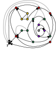
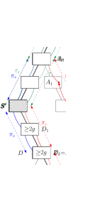
The tree of peels:
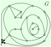
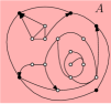
We will compute a tree that stores, roughly speaking, the hierarchy of peels for some outerface, see also Figure 1. Formally, pick a root-vertex arbitrarily, except that it should not be a cutvertex. Choose as outerface of a face incident to . Define and compute the peels of . These layers are not quite the peels of (because we start with one vertex rather than a face), and not quite the layers of a breadth-first search (BFS) tree (because we include in the next layer all vertices that share a face with vertices of the previous layer, whether they are adjacent or not). We direct each edge from the higher-indexed to the lower-indexed layer; edges connecting vertices within a layer remain undirected.
We organize the layers into a tree (the tree of peels) as follows: The root of is a node that corresponds to the entire graph ; define . For , add a node to for each connected component of . Component is part of one connected component of ; make a child of the node corresponding to in . Define to be the outerface vertices of .

Throughout this paper, we will use ‘node’ (and upper-case letters) for the elements of while we reserve ‘vertex’ (and lower-case letters) for . An interior node of is a node that is neither the root nor a leaf. We think of each node as ‘storing’ the vertices in and observe that these vertices induce a connected subgraph. Also, every vertex of is stored at exactly one node of . We need a few easy observations:
Observation 3.1 ()
The following holds for the tree of peels :
-
1.
The root of has a single child.
-
2.
Let be the nodes that store the ends of an edge . Then either is undirected and , or is directed (say ) and is the parent of .
-
3.
For any interior node of , the size is at least the fence-girth.
Proof
(1) We chose root-vertex so that it is not a cutvertex; therefore is connected and there is only one node that is a child of .
(2) For edge , let be the smallest index for which layer contains or . If both are in , then belong to the same node since they are in one connected component. If one of them (say ) is not in , then , so the edge is directed and becomes a child of since the edge ensures that is in the connected component that defined .
(3) Recall that node corresponds to a connected component of the graph obtained by deleting some of the levels. Since is not a leaf, subgraph has at least one vertex not on the outerface. Therefore, the outerface of contains a cycle that has inside and outside (since ). This cycle is a fence and all its vertices belong to . ∎
Augmenting :
It will be helpful if every vertex except root-vertex has an outgoing edge. In general, this need not hold for our input graph . We therefore augment with further edges. The following result was shown in [4]; the result there was for the peels while our definition of layers is slightly different, but one easily verifies that the proof carries over.
Claim 3.2
(based on Obs. 2 in [4]) We can add edges to (while maintaining planarity) such that for all every vertex in has a neighbour in .
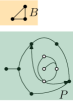
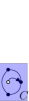
Let be the graph obtained by adding a set of directed edges such every vertex except has an outgoing edge in (Figure 1(g)). Because we only add edges between adjacent layers, the following is easily shown.
Observation 3.3 ()
The augmented graph has the same tree of peels as (assuming we start with the inherited planar embedding and outerface and use the same root-vertex).
Proof
Observe first that since we start with the same root-vertex and outerface, and only add directed edges, color=blue!50!white]FYI: We used to assume that is minimal, but I dont want to waste effort on discussing how to find this efficiently. So downgraded this to ‘add only directed edges’, which is easy to achieve. the layers are exactly the same in both and . Assume is obtained by adding just one edge (the full proof is then by induction on the number of added edges). Observe that belong to one face of since we can add edge to while staying planar. Since is connected, so is the boundary of . For any face the vertices belong to at most two consecutive layers by definition of peels; for the specific face the vertices belong to exactly two consecutive layers (say and ) since they include which are not on the same layer by construction of . So there exists in a path (along the boundary of ) that connects and and has all vertices in and .
With this, the connected components that define the tree of peels are exactly the same for both graphs. To see this, observe that when we have removed for some , then edge provides no connectivity among components that we did not have via path instead. Once we have removed , one of (and hence the added edge) has been removed from the graph, and so again does not add any connectivity. ∎
Adding edges to may decrease the fence-girth, but not the node-sizes of , which is all that will be used below. We will in the following only consider graph , so every vertex has an outgoing edge.
The detour-method:
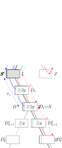
We need the following method to connect two given vertices of that are stored in the same node of (Figure 3(a) and Figure 2).
Definition 1
Fix a node of , and two vertices , as well as exit conditions which are (possibly negative) integers that will be specified by each application. The detour method at node finds a path connecting and as follows:
-
•
Initialize ; we have . We will also maintain paths (from to ) and (from to ); initially these are simply and .
-
•
If , then set to be a path from to that has distance at most . Exit with ‘success’ and return and .
-
•
If , and was the root, then return ‘fail’.
-
•
Otherwise let be the parent of . Find directed edges and , append them to paths and , update and repeat.
Since each iteration gets us closer to the root, the algorithm must terminate. If it exits successfully, say at index , then we get a walk To bound the length of this walk, the following observation will be useful:
Observation 3.4 ()
If the detour-method does not succeed at index , and is not the root, then .
color=blue!50!white]proof kicked to appendix
Proof
Recall that there are directed edges and by and that . Write for the graph induced by , and observe that must all belong to one inner face of since it bounds a connected component of the subgraph of where the peels up to have been removed. Furthermore, have neighbours both strictly inside and strictly outside (due to their outgoing edges). So there must be a simple cycle along the boundary of that contains both and . Walking along the shorter side of hence gives a walk from to of length at most . By the stopping-condition did not hold at , so this implies and the result holds by integrality. ∎
We demonstrate how to use the detour-method with the following result that will be needed later. For any node , write for the number of vertices stored at strict ancestors of .
Lemma 1 ()
Assume that for all interior nodes . For any node and any we have .
Proof
We are done if is the root or its child or a grandchild of , for then we can connect and with a path of length at most 4 by following directed edges until we reach root-vertex . So assume that has a parent , grand-parent and great-grandparent , therefore since and are internal nodes. Hence and the desired upper bound is . For ease of writing define , so the desired upper bound becomes . Apply the detour-method at , using for . If the method returns successfully at index with paths , then combining the three paths gives as desired.
So now assume for contradiction that the detour-method fails, and let (for ) be the nodes and vertices that it used; we have since the method can only fail at the root. Since the detour-method did not succeed at , color=blue!50!white]FYI: This needed a major rewrite; Obs.3.4 doesn’t hold for the root note. we did not have a path of length at most from to . But , so are connected by a path of length 0. So or . Now bound the sizes of as follows:
-
•
For , Observation 3.4 implies .
-
•
For , this bound becomes .
-
•
For , we also know since is not the root by .
-
•
Root stores one vertex .
We therefore have a contradiction:
∎

4 Outerplanarity and fence-girth
In this section, we first prove that any planar graph has outerplanarity at most where is a (user-given) integer that is supposed to be at most the fence-girth.111We use a parameter that is separate from the fence-girth since the latter can be ; to minimize the upper bound one should set to be . Then we discuss implications and lower bounds.
Separator-node :
To prove the upper bound, define the layers , augmentation and tree of peels as in Section 3. If any interior node of stores fewer than vertices, then repoert that was too big (cf. Obs. 3.1(3)) and abort. Otherwise, apply the separator theorem (Theorem 2.1) to the tree , using node-weight , i.e., the number of stored vertices. Let be a node such that any subtree of stores at most vertices; we write for these stored vertices. We know that , because the root has only one child, and .
Crucially, is close to all other nodes of . Since we will frequently need the following upper bound, we introduce a convenient notation for it.
Observation 4.1
For any node of we have .
Proof
Let be the path from to in . Every interior node of belongs to the same subtree of , and satisfies since it is neither leaf nor root. Node also belongs to and . Altogether therefore or , which implies by integrality. ∎
The overall idea of our proof is now to pick a vertex , and to argue that for all vertices . Actually, for most cases below, this will hold for any choice of .
Vertices stored in :
Let be the subtree of that contains root . For vertices in this subtree, the detour method proves the distance-bound.
Claim 4.2
Assume that . For any and any we have .
Proof
Figures 2 and 3(a) illustrate this proof. Let be the node that stores , and let be the least common ancestor of and ; this is a strict ancestor of since . Follow directed edges from to some vertex ; the resulting path has length since every directed edge gets us closer to the root. Likewise we can get a path of length from to some node (possibly ).
Now apply the detour-method with , using . This will always exit with ‘success’ at a node that is not the root, because any two vertices stored at the child of the root have outgoing edges towards the root-vertex and hence distance . Let be the paths, then has length .
To bound , consider the path from to in , which goes through , and let be the ancestors of that were visited by the detour-method. If , then by Obs. 3.4 we have for , node and the interior nodes of store at least vertices each which nodes and store at least one vertex. Therefore
hence which is at most by integrality. If then by Obs. 4.1. Either way . ∎
Vertices at descendants of :
In light of Claim 4.2, we only need to worry about vertices that are stored at descendants of . We first introduce two methods to find short paths for these in special situations. Recall that denotes the number of vertices stored at strict ancestors of node .
Claim 4.3
Assume that and . Then for any and any vertex stored at a descendant of we have .
Proof
Claim 4.4
Let be a descendant of . Let be a vertex of eccentricity at most in the connected graph (Obs. 2.2). Follow directed edges from to reach a vertex . Then for any vertex stored at a descendant of we have .
Proof
See Figure 3(c). Use directed edges to go from to a vertex along a path of length . Find a path of length at most to connect to , and then follow directed edges to get to . Combining the paths gives the desired length since .∎
Corollary 1
Assume that . Then there exists an such that for any vertex stored at a descendant of we have .
So we are done if or . Otherwise we distinguish the descendants of by their depth, using Claim 4.4 (for a carefully chosen ) for the ‘deep’ ones and the method of Claim 4.3 for the others. Define the threshold-value , call a node deep if it is a descendant of with , and call a vertex deep if it is stored at a deep node. A straightforward math manipulation gives the following upper bound.
Observation 4.5 ()
We have .
Proof
Recall that is an integer and observe that . We also know that
Therefore
which yields the result by integrality. ∎
Claim 4.6
Assume that and and . Then for any and any stored at a descendant of that is not deep, we have .
Proof
For deep nodes we show that there exists a suitable node with which to apply Claim 4.4. This is proved via a counting-argument: due to the (carefully chosen) threshold otherwise more than vertices would be stored in tree . color=blue!50!white]proof moved to the appendix
Claim 4.7
Assume that at least vertices are deep. Then there exists a descendant of (possibly itself) such that is an ancestor of all deep nodes, and .
Proof
Let be the least common ancestor of all deep nodes. This is a descendant of as well (possibly ), so enumerate the path from to as for some . We are done if for some , so assume (for contradiction) that the nodes store at least vertices each. If were deep (so ) then would store at least vertices. We also store vertices at strict ancestors at , vertices at and at least deep vertices, in total hence more than , impossible.
So is not deep, see also Figure 3(d). Since is the least common ancestor of deep descendants, therefore it must have at least two children that are ancestors of deep descendants. For , enumerate the path from to a deep descendant of as . Then for node is not a leaf and stores at least vertices, so . So for we can find vertices stored at not-deep descendants of distance from . In total these not-deep strict descendants of hence store at least vertices. As above therefore more than vertices are stored in the tree of peels, impossible. ∎
Now we put everything together.
Theorem 4.8
Let be a planar graph with vertices and let be an integer that is at most the fence-girth of . Then has a planar supergraph with . Furthermore, a vertex of with this eccentricity can be found in linear time.
Proof
Compute layers , augmentation , and tree of peels as in Section 3. Find separator-node and compute , , and the number of deep vertices. If and there are at least deep vertices, then arbitrarily fix a deep node and find node of Claim 4.7 by walking from towards until we encounter a node that stores at most vertices. In all other cases set . Pick as in Claim 4.4 applied to . Each of these steps takes linear time (we elaborate on this in Section 4.1).
Applying various cases we show that for all (which implies the result by ). This holds for all by Claim 4.2, so consider a vertex stored at a descendant of . The bound holds by Claim 4.3 if and by Corollary 1 if , so assume neither. If is not deep, then apply Claim 4.6. If is deep and there are at least deep vertices, then combine Claim 4.7 with Claim 4.4 to get the bound. The only remaining case is that , , is deep, and at most vertices are deep (so since there is a deep vertex at ). In this case, , for otherwise ’s parent would also be deep and store deep vertices. Also by . We used and picked as in Claim 4.4, so this gives as desired. ∎
Theorem 4.8 implies C2 from the introduction, for if is triangulated then necessarily and so the radius-bound holds for the input-graph as well. It also implies C1:
Corollary 2
Let be a spherically-embedded graph with vertices and let be an integer that is at most the fence-girth of . Then has fse-outerplanarity at most . Furthermore, an outerface of that achieves this outerplanarity can be found in linear time.
Proof
Without changing the spherical embedding of , compute the super-graph with ; the outerplanarity bound holds by Obs. 1.1 and the outerface can be found by picking any face incident to the vertex that achieves this eccentricity. ∎
Discussion:
Theorem 4.8 requires . We can always choose such a if is simple, but if has parallel edges or loops (which we did not exclude) then in the fixed spherical embedding the fence-girth may only be 2 or 1. We hence briefly discuss the case . Going through all proofs where or is actually used (Lemma 1, Claim 4.2 and 4.3), one sees that the results hold for if we increase the permitted distance-bound by 2. (Likewise we need to raise the permitted distance-bound in Claim 4.6 since it uses Lemma 1.) Therefore for . For , by Obs. 2.2. color=green]this paragraph could go if we need space
4.1 Run-time considerations
color=blue!50!white]this entire subsection is new and not yet very polished In this section, we elaborate on why the various steps of our algorithm can be implemented in linear time. No complicated data structures are needed for this; all bounds can be obtained via careful accounting of the visited edges.
Our first step is to compute the layers , given the spherical embedding and the root-vertex . This can simply be done with a breadth-first search as follows. Temporarily compute the radial graph, which is a bipartite with one vertex class the vertices of and the other vertex class with one vertex per face of the planar embedding; it has edges whenever a face is incident to a vertex. Then the layers are the same as the even-indexed BFS-layers of the radial graph if we start the breadth first search at root . Clearly this takes linear time to compute.
Next we must compute the augmentation . It follows directly from the proof in [4] that this can be done in linear time by scanning each face, but for completeness’ sake we repeat this proof and analyze the run-time here.
Claim 4.9
The augmentation can be computed in linear time.
Proof
We first paraphrase the proof from [4] to show that graph exists. Consider any face , and fix one vertex of that minimizes its layer-number (i.e., the index of the layer containing ). Break ties among choices for arbitrarily. For any vertex on that is not in , add an edge if it did not exist already. Clearly this maintains planarity since all new edges can be drawn inside face . Repeat at all faces to get the edges for graph . To see that this satisfies the condition, consider an arbitrary vertex in layer for some . Thus was on the outer-face of , but not on the outer-face of . It follows that some face incident to had vertices in . So our procedure added an edge from to some vertex in face that is in layer .
To find the edges efficiently, we assume that every vertex stores its layer-number. For each face we can then walk along in time to find one vertex with the smallest layer-number. In a second walk along , add all edges of that fall within face . The only non-trivial step is to check whether already existed. This could be done with suitable data structures in amortized time per edge, but the simplest approach is to not check this at all; duplicate edges in do not hurt us since we add at most edges per face and hence a linear number of edges in total. ∎
Our next step is to compute the tree of peels of , for which the main challenge is to compute the connected components after we have deleted some layers . Assume we have kept track of all edges that connect to . For each (say with ), walk along the face to the right of , from and away from , until we reach another edge for which is to the left. Repeat at the face to the right of , and continue repeating until we return to edge at the face to its left. The visited vertices form the outer-face of one connected component of , so define a new node for them, set to be the visited vertices, and make the child of the node that stored . If there are edges of left that have not been visited yet, then repeat at them to obtain the next node. At the end we have determined all nodes that together cover layer . The run-time for this is proportional to , so linear over all layers.
The next few steps (in the proof of Theorem 4.8) are to compute a number of values, and to traverse to determine all deep nodes and the number of vertices that they store; clearly this can be done in time. Likewise we can find the appropriate node to use in linear time, and finding can then be done in by using Observation 2.2 to find a central node in and then following outgoing edges until we reach . The rest of the proof is an argument that the radius is small if we use as center, but we do not actually need to perform any computation here since we already found the appropriate . So overall the run-time for Theorem 4.8 is linear, and similarly one argues the run-time for Corollary 2.
4.2 Tightness
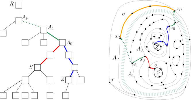
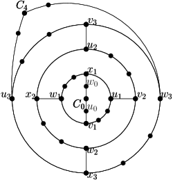
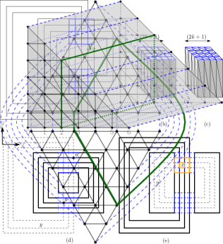
We now design graphs with large outerplanarity (relative to the fence-girth ). (These graphs actually have girth , i.e., any cycle (not just those that are fences) has length at least .) We do this first for the fixed-spherical-embedding outerplanarity, where the lower bounds hold even for . Then, for and at a slight decrease of the lower bound, we give bounds for the (unrestricted) outerplanarity. Roughly speaking, the graphs consist of nested cycles of length , with a single vertex or path inside the innermost / outside the outermost cycle, and (if desired) with edges added to ensure that all spherical embeddings have the same fse-outerplanarity. See Figure 5.
color=blue!50!white]FYI: defn of nested cycles kicked to appendix
Lemma 2 ()
For there exists an infinite class of spherically embedded graphs of girth and fence-girth for which the fse-outerplanarity is at least .
Before giving this proof, we briefly recall the definition of nested cycles. Let be a sequence of disjoint subgraphs in a plane graph . We call nested cycles if for all subgraph is a cycle that contains inside and outside. Note that and need not be cycles.
Proof
The graphs in consist of nested -cycles, with singletons as the innermost and outermost ‘cycles’. Formally, define (for ) to be a -cycle, set and to be singleton vertices, and arrange as nested cycles to obtain the (disconnected) graph with vertices (see Figure 4(a)).
We claim that (for odd) has at least peels regardless of the choice of the outerface. To see this, let be the index such that is incident to and ; up to symmetry we may assume and therefore . Let be the peels when is the outerface. Then contains , but no vertex of , so we must have at least peels (containing ). Since therefore the number of peels is at least . ∎
Theorem 4.10 ()
For there exists an infinite class of planar graphs of girth and fence-girth that have outerplanarity at least .
Proof
For the proof is very easy: Take graph from Lemma 2 and arbitrarily triangulate it while respecting the given spherical embedding. The resulting graph has a unique spherical embedding and requires (for odd) at least peels.
For graph also extends , but we must be more careful in how to add edges to keep the fence-girth big. Recall that consists of singleton , 4-cycles , and singleton , arranged as nested cycles. Enumerate each as , where for all four names refer to the same vertex. Let be the graph obtained from by adding connector-edges and for (see Figure 4(b)). One easily verifies that is bipartite, hence has fence-girth . It also is 2-connected and hence any spherical embedding can be achieved by permuting or flipping the 3-connected components at a cutting pair [13]. But any cutting pair of has only two cut-components (hence we cannot permute), and flipping the components gives the same graph (up to renaming) since is symmetric. Therefore all spherical embeddings of are the same, up to renaming of vertices. Hence for odd graph has at least peels in any planar embedding.


Now consider even, and assume that has been defined already. To obtain from it, first extend path by one vertex, i.e., it becomes a path with vertices from to . Likewise expand path by one vertex. Finally for , subdivide cycle twice, once on the part between and and once on the part between and . The connector-edges remain unchanged. Construct similarly from : expand paths and by one vertex, but subdivide (for ) only once, on the part between and . For both even and odd, graph can be obtained by subdividing edges of , hence its outerplanarity cannot be better and is (for odd) at least . Since has vertices, hence its outerplanarity is as desired. It remains to argue the girth, so fix an arbitrary simple cycle in and assume that it visits for some and no other nested cycles. If then equals and has length . If , then uses at least two connector-edges, and parts of and that connect such connector-edges; each such part has length at least and so in this case. So the shortest cycle has length at least , and this is achieved (and the cycle is a fence) at . ∎


5 Outerplanarity and Diameter
With much the same techniques as for Theorem 4.8, we can also bound the outerplanarity in terms of the diameter, as long as we permit a ‘correction-term’ of .
Theorem 5.1
Any simple plane graph with vertices has a plane supergraph with .
Proof
Compute layers , augmentation and the tree of peels as in Section 3. If then consists only of root and its unique child that stores all vertices of ; in consequence has outerplanarity at most by . So assume that and let be two nodes of with . Let be the node ‘halfway between them’, i.e., of distance from along the unique path from to in . One easily verifies that for all nodes of , otherwise would be too far away from either or since is a tree. Also note that by Obs. 3.1(2) and since is a supergraph. Finally observe that , for is an interior node by and stores at least three vertices by simplicity while at least one of is not an ancestor of and stores at least one vertex.
Pick arbitrarily. For any (say is stored at node ), we find a path from to as follows (see also Figure 3(b) and 3(c)): Let be the least common ancestor of and (quite possibly or ). Follow directed edges from and to reach vertices ; the total number of these edges is . Observe that and also . Using Lemma 1 therefore and so . ∎
Theorem 5.1 implies C3 from the introduction: The fse-outerplanarity of is at most the fse-outerplanarity of , which is at most . If is triangulated then necessarily and so . Theorem 5.2 implies that the ‘correction-term’ of cannot be avoided for the graph in Figure 6.
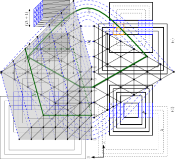
Theorem 5.2 ()
For every positive integer , there exists a triangulated graph with vertices that has diameter at most and radius at least .
Proof
Let be the triangular grid of sidelength defined as follows. Each vertex of corresponds to a point in that satisfies and . Two such points are connected if and only if their Euclidean distance is , i.e., one of the three coordinates has changed by while another has changed by . Let be a second copy of this grid, and add connector-edges for any and that have the same coordinates, and one of these coordinates is 0. We can visualize the resulting graph as lying on the triangular prism, after omitting the -coordinates, see also Figure 6. Graph has vertices as desired. It is not quite triangulated; let be obtained from by inserting arbitrary diagonals into the quadrangular faces incident to the connector-edges.
Define to be the two vertices with -coordinate . For , consider the set of all vertices that have -coordinate , and note that these form a cycle of length . Using these cycles, it is very easy to lower-bound the radius. Consider an arbitrary vertex , say it has coordinates . Since we may (up to renaming of coordinates) assume that . Let . Then each of the disjoint cycles contains on one side and on the other. So any path from to must contain at least one vertex from each of these cycles, and . So any vertex has eccentricity at least , and .
Now we upper-bound the diameter. Fix two arbitrary vertices , and assume that they have -coordinates and respectively; up to renaming . We can walk from to some vertex in steps, since for all every vertex in has at least one neighbour in . So . Vertices and both belong to , a cycle of length , and hence . Therefore and since this holds for all vertex-pairs we have . ∎
6 Remarks
While the ‘’-part of our bound in Theorem 4.8 is tight, the ‘’ part could use improvement. We can easily prove (with the same techniques as in Theorem 5.1) a bound of , but does every planar graph with fence-girth have outerplanarity ?
Also, our linear-time algorithm carefully side-steps the question of how to compute the fence-girth (it instead uses a parameter for which the node-sizes of are big enough). Testing whether the fence-girth is at most is easily done if the spherical embedding is fixed and is a constant, using the subgraph isomorphism algorithm by Eppstein [16]. But the fence-girth need not be constant and Eppstein’s algorithm does not work if the embedding can be changed. Algorithms to compute the girth [10] do not seem transferrable to the fence-girth. How easy is it to compute the fence-girth, both when the spherical embedding is fixed and when it can be chosen freely?
Acknowledgments
Research by TB supported by NSERC; FRN RGPIN-2020-03958. Research by DM supported by NSERC; FRN RGPIN-2018-05023.
References
- [1] Alam, M.J., Bläsius, T., Rutter, I., Ueckerdt, T., Wolff, A.: Pixel and voxel representations of graphs. In: Giacomo, E.D., Lubiw, A. (eds.) Proc. of the 23rd International Symposium on Graph Drawing and Network Visualization (GD). LNCS, vol. 9411, pp. 472–486. Springer (2015). https://doi.org/10.1007/978-3-319-27261-0_39
- [2] Ali, P., Dankelmann, P., Mukwembi, S.: The radius of k-connected planar graphs with bounded faces. Discret. Math. 312(24), 3636–3642 (2012). https://doi.org/10.1016/j.disc.2012.08.019
- [3] Baker, B.S.: Approximation algorithms for np-complete problems on planar graphs (preliminary version). In: 24th Annual Symposium on Foundations of Computer Science, Tucson, Arizona, USA, 7-9 November 1983. pp. 265–273. IEEE Computer Society (1983). https://doi.org/10.1109/SFCS.1983.7, https://doi.org/10.1109/SFCS.1983.7
- [4] Biedl, T.: On triangulating -outerplanar graphs. Discrete Applied Mathematics 181, 275–279 (2015)
- [5] Biedl, T., Mondal, D.: Improved outerplanarity bounds for planar graphs. In: Proceedings of the 50th International Workshop on Graph-Theoretic Concepts in Computer Science. Springer (1996)
- [6] Bienstock, D., Monma, C.L.: On the complexity of embedding planar graphs to minimize certain distance measures. Algorithmica 5(1), 93–109 (1990). https://doi.org/10.1007/BF01840379
- [7] Boitmanis, K., Freivalds, K., Ledins, P., Opmanis, R.: Fast and simple approximation of the diameter and radius of a graph. In: Àlvarez, C., Serna, M.J. (eds.) Experimental Algorithms, 5th International Workshop, WEA 2006, Cala Galdana, Menorca, Spain, May 24-27, 2006, Proceedings. Lecture Notes in Computer Science, vol. 4007, pp. 98–108. Springer (2006). https://doi.org/10.1007/11764298_9, https://doi.org/10.1007/11764298_9
- [8] Cabello, S.: Subquadratic algorithms for the diameter and the sum of pairwise distances in planar graphs. ACM Transactions on Algorithms (TALG) 15(2), 1–38 (2018)
- [9] Chan, T.M., Skrepetos, D.: Faster approximate diameter and distance oracles in planar graphs. Algorithmica 81(8), 3075–3098 (2019). https://doi.org/10.1007/s00453-019-00570-z, https://doi.org/10.1007/s00453-019-00570-z
- [10] Chang, H., Lu, H.: Computing the girth of a planar graph in linear time. SIAM J. Comput. 42(3), 1077–1094 (2013). https://doi.org/10.1137/110832033, https://doi.org/10.1137/110832033
- [11] Chepoi, V., Dragan, F.F., Vaxès, Y.: Center and diameter problems in plane triangulations and quadrangulations. In: Eppstein, D. (ed.) Proceedings of the Thirteenth Annual ACM-SIAM Symposium on Discrete Algorithms, January 6-8, 2002, San Francisco, CA, USA. pp. 346–355. ACM/SIAM (2002), http://dl.acm.org/citation.cfm?id=545381.545427
- [12] Demaine, E.D., Hajiaghayi, M.T., Nishimura, N., Ragde, P., Thilikos, D.M.: Approximation algorithms for classes of graphs excluding single-crossing graphs as minors. J. Comput. Syst. Sci. 69(2), 166–195 (2004). https://doi.org/10.1016/j.jcss.2003.12.001, https://doi.org/10.1016/j.jcss.2003.12.001
- [13] Di Battista, G., Tamassia, R.: Incremental planarity testing. In: 30th IEEE Symposium on Foundations of Computer Science. pp. 436–441 (1989)
- [14] Diestel, R.: Graph Theory, 4th Edition, Graduate texts in mathematics, vol. 173. Springer (2012)
- [15] Dolev, D., Leighton, F.T., Trickey, H.: Planar embedding of planar graphs. Tech. rep., Massachusetts Inst of Tech Cambridge lab for Computer Science (1983)
- [16] Eppstein, D.: Subgraph isomorphism in planar graphs and related problems. J. Graph Algorithms Appl. 3(3), 1–27 (1999). https://doi.org/10.7155/jgaa.00014, https://doi.org/10.7155/jgaa.00014
- [17] Eppstein, D.: Diameter and treewidth in minor-closed graph families. Algorithmica 27(3), 275–291 (2000). https://doi.org/10.1007/s004530010020, https://doi.org/10.1007/s004530010020
- [18] Gawrychowski, P., Kaplan, H., Mozes, S., Sharir, M., Weimann, O.: Voronoi diagrams on planar graphs, and computing the diameter in deterministic Õ(n) time. SIAM J. Comput. 50(2), 509–554 (2021), https://doi.org/10.1137/18M1193402
- [19] Giacomo, E.D., Didimo, W., Liotta, G., Meijer, H.: Computing radial drawings on the minimum number of circles. J. Graph Algorithms Appl. 9(3), 365–389 (2005). https://doi.org/10.7155/jgaa.00114
- [20] Grohe, M.: Local tree-width, excluded minors, and approximation algorithms. Comb. 23(4), 613–632 (2003). https://doi.org/10.1007/s00493-003-0037-9, https://doi.org/10.1007/s00493-003-0037-9
- [21] Hajiaghayi, M.T., Nishimura, N., Ragde, P., Thilikos, D.M.: Fast approximation schemes for k-minor-free or k-minor-free graphs. Electron. Notes Discret. Math. 10, 137–142 (2001). https://doi.org/10.1016/S1571-0653(04)00379-8, https://doi.org/10.1016/S1571-0653(04)00379-8
- [22] Harant, J.: An upper bound for the radius of a 3-connected planar graph with bounded faces. Contemporary methods in graph theory (Bibliographisches Inst., Mannheim, 1990) 353, 358 (1990)
- [23] Kammer, F.: Determining the smallest such that G is -outerplanar. In: Arge, L., Hoffmann, M., Welzl, E. (eds.) Proceedings of the 15th Annual European Symposium on Algorithms (ESA)). Lecture Notes in Computer Science, vol. 4698, pp. 359–370. Springer (2007)
- [24] Leiserson, C.E.: Area-efficient graph layouts (for VLSI). In: 21st Annual Symposium on Foundations of Computer Science. pp. 270–281. IEEE Computer Society (1980)
- [25] Lipton, R., Tarjan, R.: A separator theorem for planar graphs. SIAM J. Appl. Math. 36(2), 177–189 (1979)
- [26] Pramanik, T., Mondal, S., Pal, M.: The diameter of an interval graph is twice of its radius. International Journal of Mathematical and Computational Sciences 5(8), 1412 – 1417 (2011)
- [27] Shook, J.M., Wei, B.: A characterization of the centers of chordal graphs. arXiv preprint arXiv:2210.00039 (2022)
- [28] username ‘verifying’ (https://mathoverflow.net/users/82650/verifying) : Diameter vs radius in maximal planar graphs. MathOverflow https://mathoverflow.net/questions/227888/diameter-vs-radius-in-maximal-planar-graphs (2013), online; accessed June 19, 2023
- [29] Weimann, O., Yuster, R.: Approximating the diameter of planar graphs in near linear time. ACM Trans. Algorithms 12(1), 12:1–12:13 (2016). https://doi.org/10.1145/2764910, https://doi.org/10.1145/2764910
- [30] Wulff-Nilsen, C.: Wiener Index, Diameter, and Stretch Factor of a Weighted Planar Graph in Subquadratic Time. Ph.D. thesis, Department of Computer Science, University of Copenhagen (2008)
- [31] Zhang, H., He, X.: Visibility representation of plane graphs via canonical ordering tree. Inf. Process. Lett. 96(2), 41–48 (2005)