lrdcases { \newcaseslrdcases* ## {
Improved Swarm Engineering: Aligning Intuition and Analysis
Abstract
We present a set of metrics intended to supplement designer intuitions when designing swarm-robotic systems, increase accuracy in extrapolating swarm behavior from algorithmic descriptions and small test experiments, and lead to faster and less costly design cycles. We build on previous works studying self-organizing behaviors in autonomous systems to derive a metric for swarm emergent self-organization. We utilize techniques from high performance computing, time series analysis, and queueing theory to derive metrics for swarm scalability, flexibility to changing external environments, and robustness to internal system stimuli such as sensor and actuator noise and robot failures.
We demonstrate the utility of our metrics by analyzing four different control algorithms in two scenarios: an indoor warehouse object transport scenario with static objects and a spatially unconstrained outdoor search and rescue scenario with moving objects. In the spatially constrained warehouse scenario, efficient use of space is key to success so algorithms that use mechanisms for traffic regulation and congestion reduction are the most appropriate. In the search and rescue scenario, the same will happen with algorithms which can cope well with object motion through dynamic task allocation and randomized search trajectories. We show that our intuitions about comparative algorithm performance are well supported by the quantitative results obtained using our metrics, and that our metrics can be synergistically used together to predict collective behaviors based on previous results in some cases.
Index Terms:
Swarm Robotics, Swarm Engineering, Foraging.I Introduction
Swarm Robotics (SR) is the study of the coordination of large numbers of simple robots [1]. SR systems can be homogeneous (single robot type and identical control software) or heterogeneous (multiple robot types and/or control software) [2, 3, 4]. The main differentiating factors between SR systems and multi-agent robotics systems stem from the mechanisms on which SR systems are based. Historically, these were principles of biological mimicry or problem solving techniques inspired by natural systems of agents such as bees, ants, and termites [5].
The duality between SR and natural systems enables effective parallels to be drawn with many naturally occurring problems, such as foraging, collective transport of heavy objects, environmental monitoring, object sorting, hazardous material cleanup, self-assembly, exploration, and collective decision making [6, 7, 8]. As a result, SR systems are especially suited for complex tasks in dynamic environments where robustness and flexibility are key to success.
Moving beyond strictly biomimetic design, many modern SR systems have retained the desirable properties of natural systems while employing elements of more conventional multi-robot system design [9]. Those properties are:
Emergent Self-Organization. Self-organization is the appearance of structure within the swarm, which can be spatial, temporal, or functional. It arises at the collective level due to inter-robot interactions and robot decisions at the individual level [10, 11]. Once established, self-organization is generally resistant to external stimuli, and this resistance is crucial to solving complex problems with only simple agents [12, 13]. Self-organization is related to, but distinct from, the concept of emergence, which is the set difference between individual and collective swarm behavior, where the swarm behavior arises both from inter-robot interactions and individual robot decisions [14, 13]. Emergent and self-organizing behaviors are often both present in SR systems as robots collectively find solutions to a problem that they cannot solve alone [15, 12]. We term this dichotomy emergent self-organization, i.e, a two-way link between collective and individual level behaviors.
Scalability. Scalable systems are able to maintain efficiency and effectiveness as system size grows. SR systems, like natural systems, can achieve scalability to hundreds or thousands of agents through decentralized control [16]; other methods of maintaining effectiveness at larger scales include local agent communication [17, 18] and heterogeneous robots or robot roles [19, 20]. Scalability can arise directly from the design of the swarm control algorithm, but more often as a cumulative result of emergent self-organizing behaviors which are themselves decentralized and local [13].
Flexibility. Flexible systems are able to modify their collective behavior in response to unknown stimuli in the external environment, e.g., changing weather conditions [20, 21, 12]. Individual agents make decisions based on locally available information from neighbors and their own limited sensor data. This produces a spatially distributed response which arises from robot decisions as the swarm reacts and adapts to the environment. SR systems, like natural systems, can achieve flexibility in a variety of ways: pheromone trails, site fidelity, localized communication, and task allocation strategies [21, 20]. Some analytical methods, such as task allocation strategies, explicitly encode mechanisms for the swarm to collectively attempt to mitigate adversity and exploit beneficial changes in dynamic environmental conditions [21, 22]. Other methods, such as pheromone trails, rely on the plasticity of self-organizing behaviors and the development of emergent behaviors to achieve flexibility. The flexibility of such methods can therefore be coupled to, but is still distinct from, emergent and self-organizing behaviors [13].
Robustness. Robust systems are able to modify their collective behavior in response to internal, as opposed to environmental, stimuli. Such stimuli can include sensor and actuator noise, changes in system size due to the introduction of new robots, and robot failures. Robustness is therefore an emergent property of systems which demonstrate resilience to the effects of internal stimuli on individual robots [13] (e.g., losing a single robot or set of robots minimally perturbs the collective behavior of the swarm). Robustness is crucial for crossing the simulation-reality gap [6, 23]. Some SR systems handle sensor and actuator noise analytically [24, 25, 26], and can provide theoretical guarantees of robustness. Other systems rely on emergent behaviors [27] and do not provide theoretical guarantees; in such cases, robustness is coupled to, but again distinct from, emergent self-organization.
The duality between designing swarm control algorithms directly to be scalable and self-organizing, while incorporating emergent behaviors for flexibility and robustness, can be leveraged in the design of practical SR systems. First formally discussed by [28], swarm engineering seeks to design systems which are based on rigorous mathematical methods but which also possess the desirable system properties discussed above [29]. Each of these desirable properties can be designed for by answering the following design questions:
-
1.
Does the solution show emergent self-organization, indicating collective intelligence and its potential to be used in variants of the given problem?
-
2.
Does the solution scale to the current and future needs of the modeled scenario?
-
3.
Can the solution flexibly handle unknown environments or those with fluctuating conditions?
-
4.
Is the solution robust to sensor/actuator noise and population size fluctuations?
In order to answer these questions we first need a method for quantifying each of the desirable system properties with numerical calculations; to the best of our knowledge, such a methodology does not exist. The main contribution of this paper is the establishment of such a methodology and several demonstrations of its utility. Specifically, we propose:
-
1.
Metrics for SR systems properties. We present metrics for swarm emergent self-organization, scalability, flexibility, and robustness as analysis tools to assist with answering our design questions (Sections IV, V, VI and VII). Our approach is domain agnostic and serves as a starting point to develop application-specific variants. Furthermore, we establish the groundwork for more comprehensive theories of swarm behavior, because measuring system properties precisely is a necessary precursor to developing theories about what elements of a swarm control algorithm give rise to observed behaviors.
-
2.
Realistic scenario modeling. We apply our metrics to two real-world problems: indoor warehouse object transport (Section IX) and outdoor search and rescue (Section X). Through application to these complex real-world scenarios we expand the range of characteristics affecting swarm behavior which can be meaningfully studied in simulation. For example, the ability to precisely measure how different levels of sensor and actuator noise affect swarm behavior allows us to incorporate noise-generating elements of real-world problems into our scenario model and better study their effects. Without such methodology, those effects can only be studied qualitatively, which is not as useful.
A preliminary version of this paper was published in the IJCAI conference [20]. It provided metrics for scabalility, emergent self-organization, and flexibility, and evaluated them in an indoor warehouse setting. This paper extends previous work in the following ways:
-
1.
Refined metrics for emergent self-organization, scalability, and flexibility, and added metrics for robustness.
-
2.
Applying our metrics to a search and rescue scenario, in addition to an indoor warehouse scenario.
-
3.
Adding two methods that use a different way of doing task allocation to the set of swarm control algorithms which are used for comparison in each scenario.
-
4.
More thorough discussion of recent related work in swarm engineering and our metrics.
The rest of the paper is organized as follows. Section II discusses related works in swarm engineering. We discuss swarm emergent self-organization, scalability, flexibility, and robustness, and derive metrics for each in Sections IV, V, VI and VII. Section VIII describes our two real-world problems along with design constraints and candidate solutions. In Sections IX and X we apply our metrics to those two problems. We conclude with a discussion in Section XI of common themes between the two scenarios.
II Related Work
Previous work in swarm engineering can be broadly classified into two overlapping categories: automatic robot controller synthesis [23] which may guarantee collective behaviors and system properties [28, 30, 26, 31, 32], and the use of mathematical techniques to analyze and predict the collective behavior of swarms from characteristics of individual robot controllers [33, 18, 34].
A method for optimal foraging, as defined from a biological perspective, was presented in [33] based on pheromone trails. Differential equations were used to model the collective behavior of reactive robots [35] and robots with memory which perform task allocation [18]. Evolutionary techniques have also been used, and the resulting controllers shown to be capable of successfully crossing the simulation-reality gap [23, 36]; other works [37] have evolved swarm supervisors (e.g., replacements for human supervisors).
Controller synthesis via combined Lyapunov functions and control theoretic techniques can provide guarantees that the resulting swarm is “safe” (i.e., stay in a desired set of states) in problems such as area patrol, autonomous driving, and robot walking [38, 39, 40]. Similarly, ensemble dynamics filtering has been used to provably shape swarm dynamics during search and rescue [41]. Temporal logic has been used as an alternative basis for controller synthesis in scenarios where the results of robot actions are not immediately observable [28, 32] (e.g., robot motion between spatial locations), for identifying unrealizable controllers and analyzing synthesizer output [42], and automated suggestion to make unrealizable controllers realizable [43]. For a review of recent works and issues in controller synthesis, see [44].
Some previous works have considered swarm behavior in real-world settings with simulated or real robots in scenarios with non-ideal characteristics; that is, they systematically study how swarm behavior scales, exhibits flexibility, or exhibits robustness to sensor and actuator noise when ideality assumptions commonly employed during algorithm development are relaxed. Notable simulation-based examples include [20, 45] and examples with real robots include [46].
From a swarm engineering perspective, consider which of the following algorithms would have greater utility: a heuristic control algorithm with no provable guarantees but good performance on many problems of interest, or a rigorously derived control algorithm with many theoretical guarantees but relatively poor performance on problems of interest? Depending on the application parameters, stakeholders, and other factors, either algorithm may be considered the “best.”; this echoes the concept of ecological rationality, in which the actual performance of an organism in an environment is more important than its potential performance/how well adapted it is to an environment on paper.
Historically speaking, the “best” algorithm is selected through iterative refinement: testing, algorithmic study, etc. The quality of the solution depends strongly on the experience of the designer [23]. The number of design iterations can be reduced through (1) more accurate problem modeling, or (2) quantitative metrics for system properties that can be used to predict performance on variances of the problem. Previous work ([9, 47]) in swarm engineering on algorithm selection for a target application only implicitly considers the swarm properties through raw performance comparisons; a methodology capable of (1) and (2) was presented in [20] for some swarm properties.
III Metric Summaries and Preliminaries
In the sections that follow we define metric axes and derive metrics for swarm emergent self-organization, scalability, flexibility, and robustness in Sections V, IV, VI and VII. We have defined our axes and metrics to be as general as possible and applicable to almost all domains within multi-robot systems; more precise axes specific to a given domain may provide deeper insight than our definition at the expense of limited wider applicability.
The notation we use is summarized in Table I. A taxonomy of SR properties with our metric axes is in Table II, and a top-level summary of our metrics is in Table III.
| Quantity | Description |
|---|---|
| A swarm of homogeneous robots, each running . | |
| The robot control algorithm present on each robot in . | |
| The number of robots in . | |
| Two specific swarm sizes, with . | |
| A single time step of execution/the total execution time of . | |
| , | The sub-swarm () which is (is not) working on an assigned task of interest. |
| A task of interest which is working on at . may be working on multiple tasks simultaneously. | |
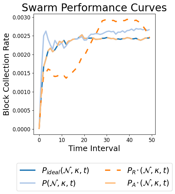
| The temporal performance curve a swarm traces out over time, measurable at each under . | |
| The temporal performance curve a swarm traces out over time, measurable at each under . | |
| Fraction of time lost to inter-robot interference within . | |
| Fraction of performance lost to inter-robot interference within . | |
| Continuous one-dimensional signal representing the ideal environmental conditions or the conditions that was developed in. | |
| Continuous one-dimensional signal representing the signed waveform of an adverse deviation from , where positive values indicate increased adversity in environmental conditions in comparison with , and negative values indicate decreased adversity. | |
| Optimal reactivity, defined as , where is a non-zero constant per dependent on the value of . | |
| Optimal adaptability curve, where the Dynamic Time Warp , regardless of . | |
| Optimal sensor and actuator noise robustness, where . | |
| Optimal population dynamics robustness, where for all , despite fluctuating . |
| Swarm Property | Property Axis 1 | Property Axis 2 |
|---|---|---|
| Emergent | ||
| Self-Organization | Spatial | Task-based |
| Scalability | Degree of cooperation | N/A |
| Flexibility | Reactivity | Adaptability |
| Robustness | Sensor & actuator noise | Population dynamics |
| Swarm Property | Notation | Summary and Intuition |
|---|---|---|
| Emergent Self-Organization | The Spatial emergent self-organization of . Computed via the degree of sub-linearity of inter-robot interference with swarm sizes. | |
| The Task emergent self-organization of . Computed via the degree of super-linearity of performance gains with swarm sizes. | ||
| Scalability | The fraction of the performance of due to (parallel) cooperation, opposed to (serial) independent action. Computed via a modified version of the Karp-Flatt metric for analyzing potential speedups in high performance computing systems. | |
| Flexibility | The proportional Reactivity of to fluctuating changes in environmental conditions over time: if conditions improve, performance improves, if conditions worsen, performance worsens. Computed via the Dynamic Time Warp (DTW) distance of from the optimal reactivity curve . | |
| The Adaptability of to fluctuating changes in environmental conditions: regardless of how conditions change, performance remains the same. Computed via the Dynamic Time Warp (DTW) distance of from the optimal adaptability curve . | ||
| Robustness | The robustness of to noisy sensors and actuators. Regardless of how noisy sensors and actuators are, the performance of should remain the same as with noise-free sensors and actuators. Computed via the Dynamic Time Warp (DTW) distance of from the ideal performance curve . | |
| The robustness of to fluctuating population sizes () over time as a result of permanent or temporary robot failures and task reallocations. Computed via the degree of sub-linear of performance decreases as the swarm population increases its variability. |
is an arbitrary performance measurement of some aspect of the behavior of : time to complete a certain number of tasks, task completion rate, etc. This formulation of swarm performance allows us to simultaneously analyze (1) cumulative performance by summing across all (scalability and emergent self-organization), and (2) temporally varying performance curves via pairwise point comparison for each (flexibility and robustness). We proceed with the following assumptions:
-
1.
for all .
-
2.
If is considered to be better than at time , then . Performance measures where smaller values are better (e.g., average time to task completion) can be made to satisfy this assumption by taking their reciprocal at each .
IV Swarm Emergent Self-Organization
IV-A Background
Within SR, no widely accepted theory of self-organizing systems exists [48, 11], in part because emergent, self-organizing swarms cannot be easily understood by studying individual parts in isolation [13]. In SR systems, interactions between components can overtake outside interactions and give rise to new emergent behaviors not predictable from component study; that is, directly from the swarm control algorithm [15, 49, 12, 13]. However, self-organization can be related to the latency of information propagation through a swarm and swarm sparseness [50], and is often synergistically coupled to emergent behaviors [13].
While many papers show evidence that their algorithms exhibit emergent behavior ([51, 47, 16]), or provide a framework for logical reasoning about emergent properties ([10, 52, 53]), a general theory of emergence remains elusive. Nevertheless, some common preconditions for self-organizing emergent behaviors have been observed [54, 13]. Let be a swarm of robots, then the preconditions are:
-
1.
Positive feedback via heuristics which promote organization at the collective level, such as reactive recruitment and reinforcement. In constrained physical environments it can lead to emergent spatial self-organization [55].
- 2.
-
3.
Random fluctuations via random walks, random task switching, etc., are necessary for collective creativity and problem solving, though they can also lead to sub-optimal collective solutions if not moderated by other properties.
-
4.
Multiple interactions between robots. Robots use information from other robots, possibly through joint environment manipulation, to choose how to act. More interactions can lead to more informed decisions.
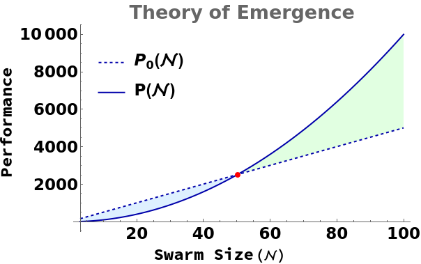
Early analyses of emergent behavior posited that a swarm of units only exhibits emergent behavior when exceeds a critical size [57]. Below this threshold, swarm attempts at self organization can negatively affect performance (Fig. 1, light blue shaded region). A more generalized definition defines emergence as the positive difference [58] (Fig. 1, shaded region), where is the amount of performance achieved by a swarm of robots, and is the amount of performance achieved by an equivalent swarm of independent agents; this intuition is also mentioned in [35, 12, 13]. In essence, emergent systems exhibit non-linearities in behavior; self-organizing systems also exhibit non-linearities as they acquire and maintain a spatial, temporal, or functional structure [13].
From these observations we develop our definition of emergent self-organization. We reject the argument that the ability of to accomplish a complex task is evidence of emergent self-organization. Consider “programmed” emergence in which robot behaviors “fit” together and directly “sum” to the desired outcome—clearly the collective behavior is easily predictable from component study, and therefore not emergent. Instead, we define emergent self-organization as the second order effects of the robot control algorithm; that is, how a complex sequence of robot-environment and robot-robot interactions can give rise to superlinear behaviors (e.g., performance gains) [12]. As an example, consider a control algorithm for cooperatively building 3D structures [59, 60]: the swarm’s ability to collectively build such structures does not in itself indicate self-organization (a single robot can also do it). Nor does it unilaterally indicate emergence: if a single robot takes seconds to build a structure, and robots take seconds to build the same structure, that is predictable from component study, since increased interference might cause a slowdown. However, if robots can build the same structure in less than seconds, then that is indicative of emergent self-organization (superlinear performance gain).
IV-B Axes Intuitions
Our two metric axes (see Table II) are based on characteristics of self-organizing systems, in which the systems are generally far from equilibrium and show an increase in order [13]. We can infer from [15, 13] that SR systems with a high degree of local interactivity should exhibit higher levels of emergent self-organization than systems with a low degree of interactivity [14, 11, 10]. From Fig. 1, we know that emergent behavior can be quantitatively measured as a super-linear increase in swarm performance as increases linearly. We argue that sub-linear increases in inter-robot interference across linearly increasing are also indicative of emergent behavior, since there may be a correlation between reduced interference and increased performance with self-organization.
We measure spatial self-organization, defined as collective optimization of inter-robot interference and movement patterns, by measuring the sub-linearity of inter-robot interference as increases. If the proportional increase in the amount of performance lost due to inter-robot interference between swarms of size and , with , is sub-linear, then self-organization has occurred. That is, has learned to leverage inter-robot interactions to become more spatially efficient with increasing . In the absence of self-organizing, random robot motions would produce approximately linear increases in inter-robot interference as the size of increases, and be in equilibrium regarding interference levels. In order for spatial self-organization to reliably arise, must be operating in a bounded space; without this restriction, a swarm will not necessarily be motivated to manage space efficiently. This restriction manifests itself in applications such as warehouses [41].
We measure task-based self-organization, defined as collective optimization of task allocation, by measuring the super-linearity of the marginal performance gain as increases [61]. If a super-linear increase in performance gained due to optimization of higher level swarm functions is observed between two swarms of size and , then emergent self-organization has occurred. That is, the swarm has learned to leverage inter-robot interactions and relationships between tasks to become more efficient with larger . In applications without a bounded operating arena, task-based self-organization is more likely to emerge than spatial self-organization, as it does not directly depend on environmental factors.
IV-C Metric Derivations
Formalizing our intuition, we define our task emergent self-organization measure as follows. We calculate (post-hoc) the number of robots experiencing inter-robot interference, instead of doing useful work, within on each timestep , denoted as . This can then be used to compute the per-timestep fraction of overall performance loss as follows:
| (1) |
Eq. 1 quantifies a swarm’s ability to detect and eliminate non-cooperative situations between agents (e.g., frequent inter-robot interference) as increases [49]. For we subtract the interference that would have occurred in a swarm of independent robots which never interfered with each other. If we compute Eq. 1 for two swarms of size , sub-linear increases in the computed value indicate that a swarm of robots is capable of emergent self-organization. We can now define our spatial emergent self-organization measure , where positive values indicate self-organization, as:
| (2) |
V Swarm Scalability
V-A Background
In recent years, swarm engineering has produced many design tools and methods for rigorous algorithm analysis and derivation of analytical, rather than weakly inductive proofs of correctness [22, 16, 31, 62, 63, 32]. Despite this, there has not been a corresponding increase in the number of robots used, which is important for tackling problems of real-world scale. Investigation of simple behaviors such as pattern formation, localization, or collective motion is generally evaluated at small scales, with 20–40 robots [64, 23, 22], and more complex behaviors such as foraging and task allocation with 20–30 robots [65, 66, 31]. Notable exceptions to this trend include [62, 6, 48, 20], which used 600, 768, 375, and 16,384 robots respectively.
While these swarm sizes may technically meet the criteria to be a considered a swarm (10–20 robots [1]), from a swarm engineering perspective they may not provide enough confidence in algorithm correctness, since studies at small scales may suffer from unmanifested theoretical and empirical scalability issues. Furthermore, reliably analyzing emergent and self-organizing behaviors during the design process is difficult at small scales since they only reliably arise at larger scales, where “larger” is problem-dependent [52].
Previous work calculated swarm scalability as (i.e., per-robot efficiency) [6]. While this measure provides insight into scalability, it is not predictive (e.g. given , we cannot plausibly estimate without retroactively charting across a range of values for ).
V-B Axis Intuition
Our metric axis (see Table II) is based on the intuition that robots in are analogous to nodes in a supercomputing system: if a job takes seconds with robots, ideally it will take seconds with robots in a perfectly parallelizable system. We adapt the Karp-Flatt metric [67] which measures the level of parallelization of a program and the plausibility of speedups if more computational resources are added, to swarm engineering, where it exposes the portion of observed performance rooted in inter-robot cooperation. Using such a metric, higher values will indicate cooperative swarms and plausible predictions of efficiency increases for larger .
V-C Metric Derivation
Formalizing our intuition, we define our scalability measure , where , using the Karp-Flatt metric:
| (4) |
In Eq. 4, the term in is the serial fraction from the original Karp—Flatt paper. Our formulation defines “speedup” as the performance gain with robots over the performance with robots, rather than over the performance with 1 robot, per the original paper. This “marginal performance gain” provides comparable results between which require a critical to perform well (i.e., sub-linear increases in performance across small ), and which have more linear increases in performance across small . Negative values for are possible, due to the fact that the original Karp-Flatt metric assumes that is a monotonically increasing function (i.e., adding more processors always gives some marginal gain), and this assumption is not valid in general for SR systems when adding more robots.
VI Swarm Flexibility
VI-A Background
Flexibility among agents within a swarm in response to environmental changes is an important aspect of their collective utility: they should be able to react to factors in the environment, such as the quality or safety of locations within it, while also not changing their behavior in response to every fluctuation [12]. Some works on flexibility compare the raw performance of swarm control algorithms under dynamic environmental conditions [21, 18] or conditions from those they were developed in [68, 69, 6]. However, the resultant claims of flexibility due to performance similarity across scenarios is strictly qualitative, due to a lack of mathematical quantification of “difference” in scenario conditions as a factor in performance comparisons.
VI-B Axes Intuitions
A swarm is considered flexible if it can self-organize to cope with a variety of non-ideal environmental conditions (defined by ) which change over time and are different than the conditions it was developed in. These changes can include the cost of performing a particular action (e.g., picking up/dropping an object in foraging), maximum robot speed (e.g., wheeled robots buffeted in variable winds in outdoor environments) or the performance of some tasks more slowly than others (e.g., carrying objects of differing weights).
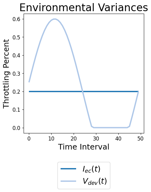
We measure swarm flexibility along two opposing axes (see Table II) in order to encompass a wide range of possible design constraints. First, its reactivity: how quickly and proportionally changes according to changes in , as shown in Fig. 2. Second, its adaptability: does not change, regardless of (i.e., consistent performance). That is, if non-ideal environmental conditions change over time, performance does not change in ideal environmental conditions, as shown in Fig. 2. Adaptive swarms minimize performance losses under adverse conditions (), and resist performance increases under beneficial deviations from , (i.e., ).
VI-C Metric Derivations
Using the results of [70], we derive temporally-aware measures quantifying the difference between expected and observed performance in arbitrary environmental conditions, and use it to calculate swarm reactivity and adaptability.
To derive the performance curve of a swarm with optimal reactivity, , we note that such a swarm will react instantaneously and proportionally whenever is non-zero. Define as a per-timestep constant representing the signed proportional difference between ideal and non-ideal conditions:
| (5) |
Then, for all , and we can now define our reactivity measure :
| (6) |
where is a Dynamic Time Warp similarity measure between two discrete curves and , based on the conclusions in [70]. We note that DTW correctly matches temporally shifted sequences of applied variance and observed performance (achieving is not possible for realistic swarms), and exhibits robustness to signal noise.
It is clear from our intuition above that in a swarm with optimal adaptability, for all . We can now define our adaptability measure :
| (7) |
where is a Dynamic Time Warp similarity measure, for the same reasons described above for .
VII Swarm Robustness
VII-A Background
Bjkernes et al. [45] show that contrary to the common assumption in SR literature, larger swarms can be less robust than smaller swarms, and argue that fundamental changes to SR system design, such as the inclusion of an artificial immune system, are required to detect and self-heal from faults. A generic framework for fault detection in robot swarms based on immunological response and peer voting was presented in [71], and showed a high level of accuracy in identifying a faulty robot in real-robot swarms, even if swarm behavior collectively changed over time. Other works in formation control [72] and decision making [73] treat robustness from the perspective of the ability of to meet its goals in the presence of malicious robots, and provide provable collective behavior guarantees, which are by their nature guarantees of emergent behavior. Availability analysis, i.e., determining what fraction of a swarm will be available on average in statistical equilibrium to work on tasks, given robot malfunction and repair rates, has investigated both independent and coupled robot malfunction rates [74].
Swarm robustness in the presence of single robot sensor malfunction was demonstrated in [4], allowing failing robots to share data with functioning robots. Swarm robustness to Gaussian noise was measured and analyzed by [26, 24] on collective swarm motion, and on obstacle detection [25]. Gaussian noise was applied to robot sensor readings in [9], and their effects studied for different variants of a foraging algorithm. The Fokker-Planck equation was derived from statistical physics for a given Langevin equation governing robot motion, including noise models, and applied to the analysis of simple phototaxis (i.e., motion towards light) behaviors [48]. Other works inject a small level of uniform or Gaussian noise (0.5–10%) to help narrow the simulation-reality gap, without performing statistical analysis [6, 66]. Many theoretic works do not incorporate noise into their models [18, 30]; exceptions include [26]. Similarly, many application oriented works do not systematically evaluate algorithms in the presence of noise; exceptions include [9, 24].
VII-B Axes Intuitions
We motivate our robustness axes by considering real world examples such as underwater, mining, and warehouses [68, 41]. In such environments, swarms may have to deal with one or more of: (1) high levels of sensor and actuator noise, (2) adversarial task re-allocation in which robots can leave a sub-swarm working on a certain task at any time, and (3) frequent robot mechanical failures. We therefore define a swarm’s robustness along two axes.
First, sensor and actuator noise robustness, or its ability to collectively adapt to temporally varying levels of sensor and actuator noise. Swarm sensor and actuator noise robustness should measure how close of remains to when affects the internal state of via sensor and actuator noise, where is the performance of with idealized, noise-free sensors.
Second, population dynamics robustness, or its ability to collectively adapt to temporal changes in the swarm size . We emphasize the collective adaptation, as our robustness definition is an emergent property. Swarm population dynamics robustness of should measure the ability to maintain the same level of performance as population size changes. As robots enter and leave over time (permanently or temporarily), they will have an inaccurate world model. Different will cope with these robots in different ways and will ultimately affect differently. We want to correlate with changes in . Building on [74], we derive expressions for the average number of robots in the system and how long a robot stays in the system, and use this to define our population dynamics robustness measure.
VII-C Metric Derivations
It is clear from our intuition above that in a swarm with optimal sensor and actuator noise robustness , for all . We can now define our sensor and actuator noise robustness measure :
| (8) |
where is a Dynamic Time Warp similarity measure, as described in Section VI for and . We compare performance curves, rather than cumulative performance values, in order to account for swarm emergent (partial) mitigation of the noise via changing behaviors.
To compute the variability of , we first derive the average amount of time a robot spends in , .
In queueing theory, queues are described by a tuple [75]. is the arrival process, which is typically Markovian, is the service time distribution, which is also typically Markovian, is the number of service channels available to service items as they leave the queue. We study the queue, in which items arrive at rate , remain in the queue for a period of time, and are serviced at rate [75]. We define three queues to model the possible sources of a temporally varying resulting from robots leaving , extending [74], as follows:
-
1.
Birth queue, , is an M/M/1 queue defined by , which models the periodic addition of robots to at rate that have been released from other tasks to join to work on task . begins with robots in it and has a finite population; that is, every robot not part of at is a member of this queue.
-
2.
Death queue, , is an M/M/0 queue defined by modeling the permanent removal of robots from as they critically malfunction or are permanently reallocated to other tasks and are removed from the swarm at rate . We treat the two cases identically. There are 0 servers in this queue, and hence . begins with 0 robots in it.
-
3.
Repair/reallocation queue, , is a birth-death M/M/1 queue defined by . models the temporary removal of robots from as they (1) non-critically malfunction, or (2) are temporarily reallocated to other tasks at rate (we treat the two cases identically), and return to to work on at rate . begins with 0 robots in it.
Assuming that (1) the service/arrival rates are constant, (2) are all independent, and (3) a robot can be at most in one queue at a time, we leverage the additive property of Poisson random variables and combine into a single M/M/1// queue, , which models the number of robots not in at .
To have a stable system, the utilization must be :
| (9) |
Depending on the relative arrival and service rates of , stability can be achieved in many different ways. Similarly, the variance of the size of can also vary greatly as robots stay in the swarm for different amounts of time on average. Using Little’s law [75] to calculate the average amount of time each robot spends in we have:
| (10) |
and the total amount of time that a robot spends not in :
| (11) |
We can now compute the amount of time a robot is not in (and therefore in ), by taking . Higher values of indicate more stable swarms, and lower values indicate more volatile swarms in which more “experienced” robots will have to work with the sub-optimal actions of less experienced robots which are newly added, have been repaired, or have finished a different task. We now define our population dynamics robustness measure by correlating with :
| (12) |
Eq. 12 measures the difference between and , weighted by swarm population variance, .
VIII Application Scenarios Overview
We examine two scenarios: indoor warehouse object transport (Section IX), and outdoor search and rescue (Section X), framed as swarm control algorithm selection problems. The scenarios span different problem domains in which SR systems have been successfully applied, and thus serve as excellent testbeds for determining the utility of our approach as an assistive tool in the development of SR systems. Both scenarios are “obstacle-free”, in that there are no predefined obstacles. However, robots act as moving obstacles to each other; this maps naturally to many SR applications in which there are no humans in the operating area due to safety concerns.
We frame our two scenarios as foraging tasks, in which robots gather objects from a finite operating arena and bring them to a central location. We include intuitions about how each controller will perform in each scenario based solely on their technical descriptions (Sections IX and X, respectively), so that we can determine to what extent our intuitions are supported by the numerical results from our metrics.
VIII-A Motivation via Modeling Scenario Characteristics
We motivate the need for insightful metrics by considering the design constraints shown below, each of which may be present or absent in specific scenarios such as the two we study in this work. Without precise numerical quantification of the effect of constraints on swarm behavior, then any evaluation of control algorithms will be strictly qualitative, and based solely on iterative refinement and engineer intuition. We show that our metrics encompass all the constraints shown below, and therefore solve the problem of modeling real-world scenario characteristics in a comprehensive way.
-
1.
Environmental Disturbances. In many cases, it may not be feasible to develop and test SR systems in the exact environmental conditions in which they will operate (e.g., space, military, disaster cleanup applications) due to cost or locality constraints [76]. Therefore, flexibility in reacting and adapting to unknown conditions is critical.
-
2.
Noisy environments. In many environments, sensor and actuator readings may not be accurate beyond the usual level of noise. Levels of noise can vary (1) depending on the robot’s current location in the operating arena, and (2) the current time (e.g., temporally varying sources). In this work, we consider a noise model in which the exact noise level is not known a priori, but its distribution is known or can be reasonably inferred. We further assume that the effects of sensor and actuator noise are spatially homogeneous and affect all sensors and actuators equally.
-
3.
Unreliable robots. All robots are fallible, due to the nature of robotic hardware. It is only a question of how often they fail and if the failure is permanent or repairable. Some prior work has considered temporary failures [74, 4]; we expand the scope by considering the effect of temporary and permanent robot failures.
-
4.
Semi-adversarial task reallocation. Given the inherent flexibility to adapt to perform different tasks efficiently, it is expected that not all robots within a swarm will be working on the same task at the same time, as different system operators dynamically reallocate robots to tasks in real-time. Previous work in swarm robotics in general, and foraging in particular, assumed that system operators will have exclusive use of the entire swarm, whatever its size is, for the task at hand (i.e., for all ) ([47, 20, 27, 66, 6]). For simplicity of analysis, we assume that all robot reallocations are independent and can happen at any time.
-
5.
Operating arena size. If the size of the arena in which will operate is known beforehand, variable swarm density is an appropriate model, in which swarms of increasing size are placed in the same arena. If the size of the arena is not known beforehand, constant swarm density is more appropriate, in which the size of the operating arena scales linearly with increasing . Our definition of swarm density loosely falls under the Eulerian continuum for swarm dynamics described in [77]. The choice of variable or constant swarm density is a critical factor in the design process. With variable density, robots in swarms with higher densities will experience more inter-robot interactions than robots in smaller swarms, thus skewing performance results. With constant density, as swarm sizes increase, the arena size also increases proportionally, greatly reducing skewing artifacts. An appropriate model needs to be chosen in either case, as swarm density, not size, is the critical factor in determining swarm emergent self-organization [58, 63].
-
6.
Object Distribution. The distribution of the objects to be gathered in the operating arena can be modeled in various ways. The most common distribution is random (Fig. 3a), in which objects are scattered uniformly in a square or circular environment [30, 58, 9, 6]. Other studied distributions include power law (Fig. 3b), in which objects are clustered in groups of various sizes [6]. When the object distribution is not known or cannot be inferred a priori, random or power law are appropriate, following empirical observations [6]. The single source distribution (Fig. 3c) has also been extensively studied [47, 20, 65, 27, 66].
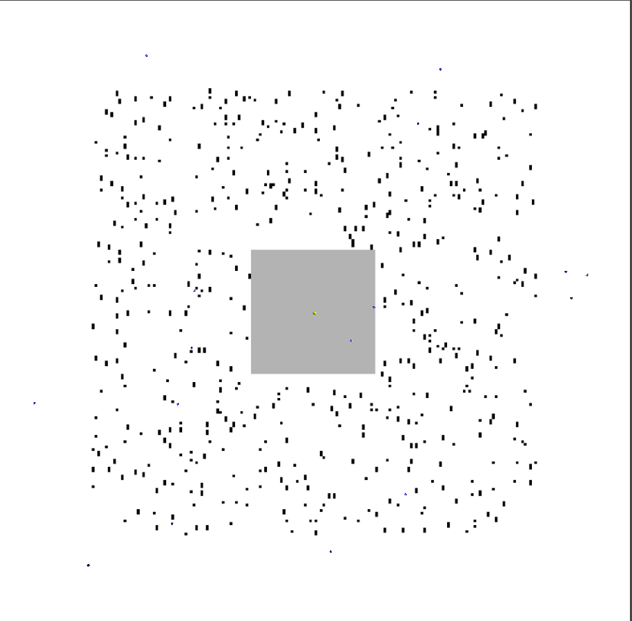
(a) Example random object distribution (scenario 1 medium warehouse, Section IX). 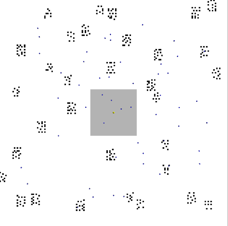
(b) Example power law object distribution (scenario 2, Section X). 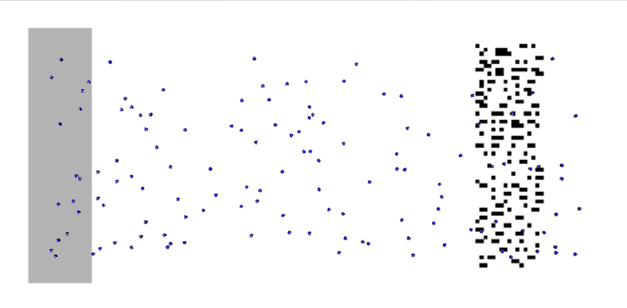
(c) Example single source object distribution (scenario 1 small warehouse, Section IX). Figure 3: Examples of foraging distributions. The nest is dark gray, objects are black, robots dark blue, and the yellow blobs are lights above the nest which robots use for phototaxis. -
7.
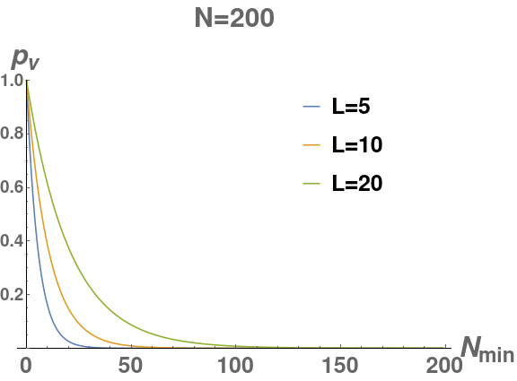
Minimum collective performance. In SR systems with task reallocation and robotic failures, a common design constraint is a minimum performance that must meet in statistical equilibrium, as fluctuates. We use the notion of swarm availability, and define as the probability that robots from a swarm of size are allocated to task at time (for a derivation, see [74]):
(13) Using Eq. 13 we can now solve for either:
-
•
, obtaining a ratio that the rates of robots entering/leaving must satisfy if are specified.
-
•
A range of achievable , given the rates of robots entering/leaving , and a range of values (see Fig. 10a for examples of this analysis).
-
•
VIII-B Candidate Algorithms ()
We have selected four state-of-the-art foraging swarm control algorithms, which in our notation we indicate with . Videos for each with different spatial distributions of the swarm are included in the multimedia accompaniment to this paper, to provide intuitive grounding of the behavior of each algorithm111https://www-users.cs.umn.edu/~harwe006/showcase/tro-2021. We selected these algorithms because they use common paradigms for foraging algorithms, from simple reactive random walks to more complex methods with theoretical bases which do task allocation. Comparative analysis across such a wide spectrum of complexity using our metrics will constitute a significant “stress test.” If they provide predictive insights, we will have strong empirical evidence that they capture underlying elements of swarm behavior.
-
•
Correlated Random Walk (CRW). Robots do a correlated random walk, which is a random walk in which the direction of the motion at each step depends on the direction of the previous step [78], until they acquire an object, which they then transport to the nest using phototaxis, i.e., motion in response to light. Robots do not reallocate tasks, i.e., they always do the same task, and have no memory (reactive algorithm). Similar controllers can be found in [35, 11].
-
•
Decaying Pheromone Object (DPO). Robots track objects they have seen using exponentially decaying pheromones [6, 27], and determine the “best” object to acquire using derived information relevance. Robots do not perform dynamic task allocation (i.e., always perform the same task). Similar controllers can be found in [33].
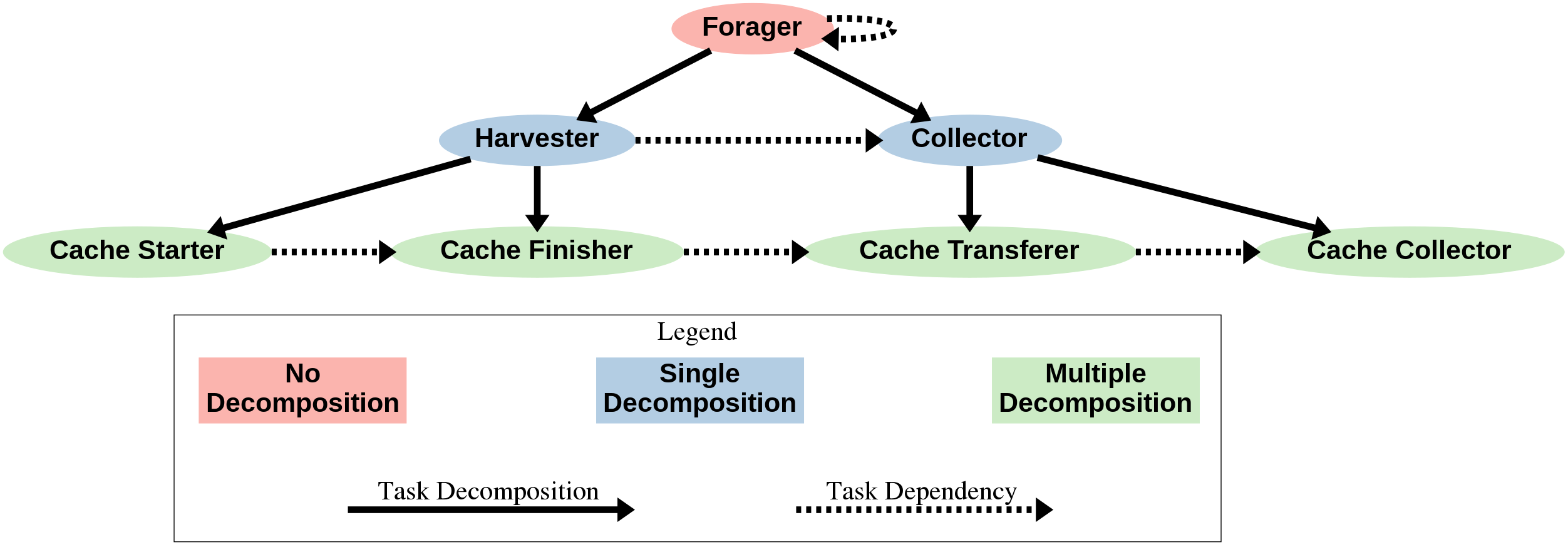
Figure 4: Task decomposition graph for the foraging task. The set of red and blue tasks correspond to a scheme in which robots do the whole task or 1/2 task (single decomposition option). The set of red and blue and green tasks correspond to a scheme in which robots do the whole task, 1/2 task, or 1/4 task (multi-decomposition option). By decomposing the task into multiple parts, there are now task dependencies between the parts, which the swarm has to collectively learn. -
•
STOCHM. Robots stochastically allocate tasks using the STOCH-N1 algorithm [27], a stochastic choice depending on the location of the most recently executed task within the graph of tasks available to each robot (Fig. 4). From Fig. 4, STOCHM robots can allocate any of the red or blue tasks, which are: (1) the entire task, Forager, retrieving an object and bringing it to the nest, (2) the first half of the task, Harvester, retrieving an object and bringing it to a static intermediate drop site (cache), or (3) the second half of the task, Collector, picking up a block from a cache and bringing it to the nest.
-
•
STOCHX. Robots also use the STOCH-N1 algorithm on the graph in Fig. 4. However, they can now choose red, blue, or green tasks, i.e., they can exploit existing caches and perform tasks related to dynamically creating new caches. The new available tasks are: placing a block somewhere to start a new cache, Cache Starter, placing a block next to a started cache to finish creating it, Cache Finisher, transferring a block between two caches, making progress towards the nest, Cache Transferer, and picking up a block from a cache and bringing it to the nest, Cache Collector. A similar algorithm for mobile caches was developed in [19].
VIII-C Experimental Framework
The experiments described in this paper have been carried out in the ARGoS simulator [79]. We employ a dynamical physics model of the robots in a three dimensional space for maximum fidelity, even if robots are restricted to motion in the XY plane, using a model of the marXbot developed by [80]. For all the experiments we average the results of 192 experimental runs of seconds. We utilize SIERRA222https://github.com/swarm-robotics/sierra.git to automatically generate simulation inputs, run experiments, and generate the graphs seen in this paper.
IX Scenario 1: Indoor Warehouse
This scenario is inspired by the use of robots in Amazon warehouses, in which SR system designers have to select a control algorithm to be deployed in a small () and a medium () warehouse of an order fulfillment company. The company has just expanded from a previous small warehouse, where they had 50 robots divided into 10 teams of 5, with each team assigned to assist with filling a given order.
After some preliminary analysis, the company believes that sufficient throughput can be maintained with robots in the small warehouse, but do not know how many robots will be needed in the medium warehouse.
| Intuitions | |
|---|---|
| CRW | • Modest spatial self-organization compared to other algorithms due to the efficiency of random motion in reducing interference. • Moderate reactivity and adaptability as a memory-less algorithm. |
| DPO | • Low spatial self-organization compared to CRW swarms because of competition at collectively learned locations of foraging targets. • Low reactivity and adaptability because is affected by changing environmental conditions but cannot substantially change behavior. |
| STOCHM | • Suffers from congestion near the locations of static caches, which may outweigh the self-organization possible due to multiple tasks. • Low self-organization because algorithm complexity and spatial cache requirements make learning through interaction in spatially constrained environments difficult. • More flexible than DPO due to the presence of caches to help regulate traffic, and the maintenance of the caches by an outside process independent of swarm behavior. • Less scalable than CRW and DPO because it balances exploitation and exploration of the search space. |
| STOCHX | • High levels of self-organization, greater flexibility, and population dynamics robustness via dynamic cache usage. • Algorithm complexity and spatial cache management make learning in spatially constrained environments difficult, so high task-based self-organization only expected in less constrained environments. • Lower raw performance than other algorithms because has to do additional work on dynamic cache management (e.g., exploration vs. exploitation of the environment). • Less scalable than STOCHM because the solution space is larger. |
IX-A Design Constraints
This scenario, or variants of it, has been studied by [47, 27, 66, 9]. Given the company’s description of their scenario, we define the following design constraints:
-
•
: Measures the rate of object collection; more efficient gather more objects per on average.
-
•
Operating arena: Fixed sizes (, ) with variable swarm density.
-
•
Object distribution: Single source for the small warehouse, and random for the medium warehouse.
-
•
Environmental disturbances: Periodic events such as shift changes and deliveries may occur, which we model as square waves, applying throttling functions to the maximum robot speed while carrying an object. This models increased congestion or additional computational time needed to plan safe trajectories in the presence of unknown dynamic obstacles while transporting goods.
Given that the frequency and disruption of the disturbances is unknown, we test throttling levels , and set the frequency , modeling periods of intense disruption that appear roughly every 1.4 hours.
-
•
Sensor and actuator noise: Given the tightly controlled indoor environment, there are no unexpected sources of sensor or actuator noise; precise indoor localization methods may also be available. However, no SR system is noise free, so we will investigate the effect of minor levels of Gaussian noise with .
-
•
Task reallocations: Given that robots will work alongside humans in both warehouses, we assume that human employees (or a centralized warehouse AI) can reallocate robots at any time as workloads evolve throughout the day. We do not have an estimate of how often this will occur from the company’s problem description, but given that , and 50 robots are available, we can compute the reallocation rates using Eqs. 13, 9 and 10 for the small warehouse, and extrapolate for the medium warehouse as needed.
-
•
Minimum collective performance: Achieved by robots for all in the small warehouse, which we extrapolate for the medium warehouse, .
-
•
Robot reliability: Given the tightly controlled indoor environment and assumed regular maintenance of robots, the overall robotic temporary failure, repair, and permanent failure rates should be negligible, and we set and , as is fixed throughout operation.
We use a arena with a single-source object distribution for the small warehouse, and a arena with a random object distribution for the medium warehouse, modeling smaller and larger scale order fulfillment operations, respectively. We use the intuitions in Table IV and perform a comparative analysis of the swarm properties, i.e., emergent self-organization, scalability, flexibility, and robustness of the candidate algorithms described in Section VIII-B to determine if our intuitions are supported by our numerical metric calculations. We omit results where no statistically significant differences are observed, or where the observed trends are the same as those for the shown warehouse.
IX-B Emergent Self-Organization Analysis


In Fig. 5a, the level of spatial self-organization remains relatively constant across all swarm sizes, indicating that each is able to manage increasingly restricted space reasonably well. The small arena size restricts the ability of swarms to learn task parameters by conflating beneficial inter-robot interactions with excessive collision avoidance, and there are no statistically significant differences in the spatial self-organization among the more complex STOCHM and STOCHX algorithms. We see statistically significant differences between CRW and the other algorithms in the small warehouse, however, as its purely reactive nature is relatively unaffected by the conflation.
Spatial self-organization emerges due to sufficiently large perturbations of robot exploratory random walks via interference by robots returning to the nest with objects and the otherwise random motion of the swarm for CRW. In more spatially constrained situations, DPO robots are less random, but compensate for this with memory. STOCHM and STOCHX robots have additional fluctuations due to their stochastic task allocation policies. Overall, these observations demonstrate the importance of the random fluctuations system property necessary for self-organization to occur, as discussed in Section IV-A, and that in spatially constrained environments self-organization can arise even in less “intelligent” algorithms due to the high levels of inter-robot interaction. This suggests that algorithmic randomness is the most important factor in emergence, together with swarm density, which was shown in previous work to be critical to develop self-organization [58].
From Fig. 5b we see few statistically significant differences between the level of spatial self-organization for CRW, DPO, and STOCHM. In this less spatially constrained environment, the swarm must collectively learn more from fewer interactions (i.e., there is less conflation between different types of inter-robot interactions), demonstrating the importance of the multiple interactions system property necessary for self-organization to occur, as discussed in Section IV-A. As expected, the complex STOCHX algorithm is the most adept at doing this via its dynamic use of caches, and obtains a near linear scaling in self-organization as is increased.
IX-C Scalability Analysis


From Fig. 6, we see much tighter confidence intervals for the simpler CRW and DPO algorithms, and broader intervals for STOCHM and STOCHX, indicating that while more “intelligent” algorithms have the potential to be highly scalable, their scalability is also more stochastic than simpler algorithms. This is in agreement with the intuitions laid out in Table IV: more complex algorithms balance exploring the solution space with exploiting the current solution, resulting in reduced performance and scalability, while simpler algorithms perform more exploitation of the current solution than exploration, resulting in increased performance and scalability.
Between Fig. 5 and Fig. 6 we see strong orthogonality between self-organization and scalability/performance: algorithms which are more “intelligent” are less reliably scalable, though they can be more scalable than less intelligent algorithms. Previous work [27] has shown that STOCHX outperforms the other algorithms in foraging scenarios more conducive to the emergence of strong traffic patterns. The random foraging environment of the medium warehouse is much more adverse, leading to the observed lower performance and scalability. This difference demonstrates the interaction between scenario characteristics and swarm dynamics, the necessity of accurate modeling and thorough analysis when designing SR systems, and the importance of matching algorithms to environments to which they are naturally well-suited.
IX-D Flexibility Analysis


In Figs. 7 and 8, we see more statistically significant differences between algorithms in reactivity and adaptability for the medium warehouse than for the small one, which is likely due to the conflation of the experimental variables for inter-robot interference and environmental adversity in the small warehouse, as discussed in Section IX-B. We also see further evidence of synergy between our measures in the correlation between the relative levels of spatial and task-based self-organization and flexibility.
STOCHM and STOCHX swarms have the highest levels of self-organization (Fig. 5), and the highest reactivity and adaptability as well for more disruptive . The DPO algorithm, while more complex than CRW, is not as reactive or adaptive, demonstrating that adding cognitive capacity to a given algorithm is not guaranteed to make the swarm more flexible. DPO swarms are unable to substantially react to changing environmental conditions because they are fundamentally unable to alter their behavior, which is compounded with increased congestion at shared resources, which manifests as a lack of “intelligence” in changing environmental conditions.
STOCHM performs better due to the more complex task allocation distributions, and STOCHX swarms, as expected, are generally the most reactive and adaptive of all evaluated algorithms. Both STOCHM and STOCHX are also cognitive, suggesting that it is possible to design a complex, cognitive algorithm which is just as flexible as a reactive algorithm—an important insight during the design process. More work is needed to further explore this relationship, but our results suggest that there is a threshold of emergent self-organization for cognitive algorithms which must be met in order to obtain collective performance which consistently outperforms that of simpler biomimetic algorithms.
In the medium warehouse (Figs. 7b and 8b), because the relative levels of inter-robot interference are lower, we see much more consistent trendlines of approximately the same slope for STOCHX swarms, indicating that such swarms are sufficiently “intelligent” to maintain nearly identical marginal reactivity to increasingly adverse environmental conditions (i.e., very small slopes). Other algorithms, having less “intelligence,” show decreasing marginal reactivity (i.e., increasing slopes).
IX-E Robustness Analysis


For the small warehouse in Fig. 9a, the CRW and STOCHX algorithms generally show statistically equivalent robustness. Of all the candidate algorithms, CRW is the least reliant on the accuracy of sensors/actuators of all algorithms, while STOCHX has a high level of self-organization—both equivalent means of achieving robustness to sensor and actuator noise. DPO and STOCHM likewise are not statistically different in terms of sensor and actuator noise robustness, except at higher . We see a clearer separation between algorithms in the medium warehouse in Fig. 9b, again likely due to the reduced conflation between different types of inter-robot interactions. In both Figs. 9a and 9b, we also see strong evidence of “phase transitions” of the behavior of all algorithms with . The transition is much more pronounced for DPO and STOCHM, in which the ability of these algorithms to handle injected noise begins to break down—a crucial insight in the design process.
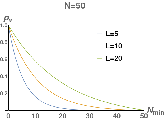


To analyze population dynamics robustness, we use for the small warehouse, per the company’s specification, and Eq. 13 to solve for , given desired steady state , shown in Fig. 10a. Given that sufficient performance can be achieved (per scenario specification) with robots for any algorithm, we see that this corresponds to , meaning that approximately 40% of the time all 5 robots of a given team were available to work on filling an order. For the medium warehouse, we use and , extrapolating from the company’s specification, and solve for in the same manner, shown in Fig. 10b. With , the availability curves drop off much more steeply, and we must have larger team sizes to achieve the same level of availability as the small warehouse.
We again see the same dichotomy between STOCHM/DPO and STOCHX/CRW in the small warehouse in Fig. 11a for higher population variances: the emergent self-organization of the STOCHX algorithm makes it the most robust to fluctuating swarm sizes, while other algorithms struggle. We speculate that the dynamic use of caches by STOCHX allows additional information about the current swarm task distribution to be encoded into the environment, which can then be partially recovered by returning/new robots, per our intuition. In Fig. 11b, we see much stronger evidence of synergy between our metrics: the relative ordering mirrors the level of emergent self-organization, with the caveat of a possible lack of statistically significant differences between STOCHM and CRW.
We have discussed swarm self-organization, scalability, flexibility, and robustness for the warehouse scenario for all . It would now be up to the company to take our results and determine which of the four main swarm properties are most important to them to make a final algorithm decision.
Overall, we see strong evidence in this section’s analyses of the synergistic nature of our metrics for SR system properties: trends within and between curves on graphs of each can be intuitively explained, and easily mapped back to the technical specifications of a given method in ways that are not evident from raw performance curves. We have observed strong correlations between emergent self-organization, scalability, flexibility, and robustness, and our intuitions in Table IV.
X Scenario 2: Outdoor Search and Rescue
This scenario is inspired by the human-swarm interaction discussion in [8], in which we as SR system designers are tasked with choosing an appropriate control algorithm for an outdoor search and rescue task. The system will be deployed in disaster zones/military conflict zones in a fully autonomous fashion as a first response measure, to assess a given outdoor environment and to search for “objects” of interest within the environment. These objects can be unconscious civilians trapped in rubble, or places of utility line breaks (e.g., gas lines), which need to be quickly discovered and reported to human responders for further investigation in order to minimize loss of life and further infrastructure damage. Some civilians may be conscious and trying to make their way out of the disaster zone or help others, in which case they need to be found and guided to the nearest safe zone. Similarly, the location of utility line breaks may appear to “move” as robot onboard sensing is not powerful enough to provide precise coordinates in potentially occluding environmental conditions.
Moderate levels of robot losses are expected due to the instability of the environment, despite hardened robotic hardware. Therefore, relatively large is required to ensure the success of the mission; we evaluate all algorithms with (12 used for baseline reference), and show raw performance results with . The selected control algorithm needs to be highly scalable and intelligent, so that it can efficiently adapt to a wide range of problem scales and unknown environmental conditions, and provide stable performance across highly volatile environmental conditions.
| Intuitions | |
|---|---|
| CRW | • No negative effects from moving targets, strong robustness to fluctuating populations, and high flexibility because of lack of memory. • Robustness to sensor noise because of minimal sensor usage. |
| DPO | • Lower levels of self-organization than CRW, because its world model assumes static object locations. • Low robustness to sensor and actuator noise because of high sensor usage. • Minimal population dynamics robustness, due to dependence on accurate world models for efficiency. • Low flexibility due to lack of ability to change allocated task. |
| STOCHM | • Poor self-organization and population dynamics robustness due to static cache usage with moving targets; minimal information about task distribution can be encoded into caches because they are maintained by an outside process. • Low population dynamics robustness due to dependence of behavior on accurate robot world models, but higher than DPO, because some information about the world model carried by robots is now encoded in the environment, and the ability to choose from multiple tasks should also improve collective re-convergence to steady-state. |
| STOCHX | • Modest self-organization due to dynamic cache usage and highly flexible task allocation distribution despite moving targets; better than STOCHM because caches can be created and depleted to help offset target motion. • Modest population dynamics robustness, flexibility due to the ability to encode the current task distribution into environmental state for inexperienced robots to find via caches (or a lack thereof). |
X-A Design Constraints
This scenario, or variants of it, has been studied by [81, 7]. We define the following design constraints:
-
•
: measures the rate at which objects are picked up for the first time; more efficient will discover more objects faster.
-
•
Operating arena: Variable size with constant swarm density; size of the arena in which targets can be found is not known beforehand. Given the limited sensing capabilities of the robots, and the anticipated robot losses due to malfunction or environmental issues, relatively large swarm sizes should be tested.
-
•
Object distribution: Not known a priori, so random or power law are appropriate models; we choose power law. Objects can move randomly over time; it is not known how often this happens so we evaluate performance with .
-
•
Environmental disturbances: Potentially large gradually evolving environmental disturbances during swarm operation, such that the swarm operating conditions will change from favorable to unfavorable or vice versa, and back again throughout swarm operation (e.g., a passing storm, windy conditions, change in visibility, etc). We apply throttling functions to the maximum robot speed during operation, and use a sinusoidal disturbance model with throttling amplitudes and frequency , modeling cyclically shifting environmental conditions roughly every 2.75 hours.
-
•
Sensor and actuator noise: Environmental disturbances may occur, such as clouds interfering with localization, fluctuating lighting conditions interfering with perception, etc. Given our hardened robotic hardware, we select a Gaussian noise model with as an appropriate model, and test with .
-
•
Robot reliability: Environmental disturbances and the general unpredictability of operating in an outdoor environment may give rise to software or hardware artifacts which will cause robots to fail permanently, so we test .
-
•
Task reallocations: No unexpected task reallocations, due to the time sensitivity of the application, so we set .
We develop the intuitions shown in Table V, and perform a comparative analysis of the emergent self-organization, scalability, flexibility, and robustness of the candidate described in Section VIII-B to determine if our intuitions are supported by our numerical measurements. We omit results where no statistically significant differences are observed.
X-B Emergent Self-Organization Analysis


In Fig. 12, we see a strong dichotomy: STOCHX and CRW swarms show consistent levels of self-organization across swarm sizes for both high and low rates of target motion, while the self-organization of DPO and STOCHM swarms is much more sensitive to swarm sizes across both target motion rates. As swarm sizes increase, it naturally becomes easier to find moving targets through sheer numbers rather than intelligent algorithm design. At smaller swarm sizes, STOCHX exhibited the strongest trends (marginally), and was therefore able to overcome some of the world model errors introduced by target motion through the emergence of specialized task allocation distributions, dynamic cache usage, and bucket brigading, while the (partially) random walk used in CRW also proves an effective strategy, despite its simplicity.
DPO relies heavily on static target locations, while STOCHM relies on both static target and static cache locations. As a result, much of the learning of STOCHM swarms to utilize caches is wasted due to the unconstrained nature of the environment and target motion. Overall, the strategies used by these algorithms are much less effective when compared with STOCHX and CRW, as we would intuitively expect.


From Fig. 13, we observe a negative correlation between emergent self-organization and performance, in contrast to [27]. This suggests that the correlation between self-organization and performance is highly dependent on the nature of the environment and that in dynamic or extremely adversarial environments, less “intelligent” algorithms may perform better, as we would expect.
X-C Scalability Analysis
The extremely adverse power law object distribution in this scenario is not conducive to self-organization because of its irregular block clusters. In combination with a constant swarm density and target motion this leads to no statistically significant differences in scalability between the algorithms. This result is in contrast to [27], in which differences in emergent self-organization were positively correlated with statistically significant differences in scalability. This again suggests that positive correlation only holds in static environments, and that in dynamic and adversarial environments, “intelligence” plays a minimal role in determining scalability.
Having analyzed the effect of target movement rate, we set a moderate rate of to simplify the rest of our analyses.
X-D Flexibility Analysis


In Fig. 14a, we see the same dichotomy observed in Sections X-B and X-C: CRW and STOCHX are the most reactive algorithms, and DPO and STOCHM are the least. However, this dichotomy only emerges for higher levels of environmental disturbances; for smaller levels, the algorithms are largely statistically equivalent. Overall, as expected, the CRW and STOCHX algorithms are the most reactive, due to their memory-less nature and ability to dynamically utilize caches, respectively. DPO and STOCHM, which rely on static object and cache locations, are much less reactive.
In Fig. 14b, we see fewer significant differences between algorithm adaptability, regardless of the level of environmental disturbance, with the exception of CRW showing significant differences with DPO and STOCHM for higher levels of environmental disturbance. In the presence of randomized target motion, we expect it to be difficult for algorithms to also adapt to changing environmental conditions. In this instance, the memory-less CRW algorithm is the only algorithm able to statistically differentiate itself from the other evaluated algorithms.
X-E Robustness Analysis


In Fig. 15b, we see identical trends for each individual , as well as identical trends between . The robustness of CRW and STOCHX swarms to sensor and actuator noise is statistically identical in most cases for increasing . For CRW swarms this is likely due to their low reliance on the accuracy of sensors and actuators during operation: the more reliant a swarm control algorithm is on accurate sensor and actuator information, the less robust it will be to adverse environmental conditions which negatively affect sensors and actuators. For STOCHX swarms this is likely due to their ability to be flexible and switch tasks dynamically to attempt to mitigate the noise (e.g., less transporting of objects over long distances, which is more prone to localization errors).
DPO, STOCHM, and STOCHX swarms have noticeably lower robustness for larger values of , and undergo phase changes at , with the overall robustness dramatically dropping for larger . This is the inflection point at which the combination of increasing noise and moving objects overwhelms the swarm’s cognitive ability to compensate; it occurs at much lower for STOCHM swarms than those for DPO and STOCHX, due to their usage of static caches as they attempt to adapt.
In Fig. 15a, CRW swarms exhibit a high level of population dynamics robustness, due to their memory-less nature; similarly for STOCHX swarms with their ability to encode the current task distribution into environmental state for inexperienced robots to find via caches. DPO and STOCHM, lacking such abilities, have much lower robustness. For the omitted graph with , statistically identical responses to pure death dynamics follow directly from our intuition: with large swarm sizes, the loss of an individual robot affects the swarm’s overall progress on its task much less. However, this observation is likely tied to the extremely adversarial nature of the scenario, and we would reasonably expect differences to emerge in a more favorable environment.
Our results in this section suggest strong synergy between our robustness and flexibility measures, similar to what was observed for the first scenario. We have again seen quantitative confirmation of our intuitions for each through our derived metrics for each of the swarm properties of self-organization, scalability, flexibility, and robustness. It would now be up to project managers to take our recommendations and make a final decision. However, our results suggest that the STOCHX algorithm is, on the whole, best suited to the outdoor search and rescue application.
XI Discussion
The application of our proposed metrics to the object transport and search-and-rescue scenarios in Sections IX and X provides a weakly inductive proof of their correctness and utility within the foraging domain, if not more broadly. Despite fundamental differences in characteristics between scenarios, our metrics were still able to expose the same underlying traits of each controller which originated in our intuitions (Tables IV and V). We saw similar dichotomies emerge between the CRW/STOCHX and DPO/STOCHM controllers, and that while more “intelligent” algorithms might not be the most scalable or highly performing, depending on environmental conditions and scenario characteristics, they were reliably more flexible and robust. This is an important insight for swarm engineers to consider when designing SR systems, and is not easily obtainable from simply comparing raw performance results.
Furthermore, our methodology provided a clear mapping from results back to our intuitions for the evaluated algorithms in both scenarios. We therefore argue that our proposed metrics are insightful tools for making theoretically grounded decisions on algorithm selection from high level algorithm descriptions, such as those we presented in Section VIII, for many real-world applications beyond the foraging tasks discussed here, and they should be included in the swarm engineer’s toolbox.
Our general definition of is an arbitrary performance measure, and by basing all of our measures on it, it is easy to analyze other foraging algorithms. For example, in analyzing a partial differential equation behavioral prediction approach to foraging, we could define as the number of robots carrying objects back to the nest [35], or how well population fractions engaged on various tasks are balanced [18]. In [19], the use of dynamic depots could lead to a logical definition of as the average load level or wait time of each depot.
We emphasize again that the definitions of our measures were intended to be application agnostic; it is possible to define more precise definitions specific to a given application. For example, one could define emergent self-organization according to the rate at which something happens (e.g., rate of construction progress [59]), with the rate of a baseline algorithm with a “random” construction strategy subtracted. Such a definition would have more utility in the realm of autonomous construction than our definition, but would have little outside of it; our measures, while not as precise as application-specific ones, can be used broadly across many sub-fields in swarm robotics.
XII Conclusions and Future Work
We have presented a set of metrics for more precise characterization of swarm emergence, scalability, flexibility, and robustness in order to provide mathematical tools to support the iterative design process of SR systems within swarm engineering. We demonstrated the utility of our methodology in the context of two different foraging tasks under various design constraints, and have shown that they provide intuitive insight into recommending a given method for a scenario.
Next steps in this research include applying our methodology to other domains within SR, such as collective transport, pattern formation, etc. We are also interested in combining our derived measures with predictive modeling and investigating how analytical derivations of and from scenario input parameters can be leveraged to predict swarm emergent self-organization, scalability, flexibility, and robustness from fundamental principles, and have begun investigating this in our ongoing work.
In order to facilitate future research and collaboration, the code used for this research is open source, and can be found at https://github.com/swarm-robotics/fordyca and https://github.com/swarm-robotics/sierra.
References
- [1] E. Şahin, “Swarm robotics: From sources of inspiration to domains of application,” in Swarm Robotics, ser. LNCS 3342. Springer, 2005, pp. 10–20.
- [2] M. Dorigo et al., “Swarmanoid: A novel concept for the study of heterogeneous robotic swarms,” IEEE Robotics Automation Magazine, vol. 20, no. 4, pp. 60–71, 2013.
- [3] Y. Rizk, M. Awad, and E. W. Tunstel, “Cooperative heterogeneous multi-robot systems: A survey,” ACM Comput. Surv., vol. 52, no. 2, Apr. 2019.
- [4] R. K. Ramachandran, N. Fronda, and G. S. Sukhatme, “Resilience in multi-robot target tracking through reconfiguration,” in 2020 IEEE International Conference on Robotics and Automation (ICRA), 2020, pp. 4551–4557.
- [5] T. H. Labella and M. Dorigo, “Division of labor in a group of robots inspired by ants’ foraging behavior,” ACM Trans. on Autonomous and Adaptive Systems (TAAS), vol. 1, no. 1, pp. 4–25, Sep. 2006.
- [6] J. P. Hecker and M. E. Moses, “Beyond pheromones: evolving error-tolerant, flexible, and scalable ant-inspired robot swarms,” Swarm Intelligence, vol. 9, no. 1, pp. 43–70, 2015.
- [7] V. Kumar and F. Sahin, “Cognitive maps in swarm robots for the mine detection application,” Proc. IEEE Int’l Conference on Systems, Man and Cybernetics, vol. 4, pp. 3364–3369, 2003.
- [8] D. Carrillo-Zapata, E. Milner, J. Hird, G. Tzoumas, P. J. Vardanega, M. Sooriyabandara, M. Giuliani, A. F. T. Winfield, and S. Hauert, “Mutual shaping in swarm robotics: User studies in fire and rescue, storage organization, and bridge inspection,” Frontiers in Robotics and AI, vol. 7, p. 53, 2020.
- [9] E. Castello, T. Yamamoto, F. D. Libera, W. Liu, A. F. Winfield, Y. Nakamura, and H. Ishiguro, “Adaptive foraging for simulated and real robotic swarms: the dynamical response threshold approach,” Swarm Intelligence, vol. 10, no. 1, pp. 1–31, 2016.
- [10] A. F. T. Winfield and J. Sa, “On formal specification of emergent behaviours in swarm robotic systems,” Science, pp. 363–371, 2005.
- [11] A. Galstyan, T. Hogg, and K. Lerman, “Modeling and mathematical analysis of swarms of microscopic robots,” in Proceedings 2005 IEEE Swarm Intelligence Symposium, 2005. SIS 2005., 2005, pp. 201–208.
- [12] E. R. Hunt, “Phenotypic plasticity provides a bioinspiration framework for minimal field swarm robotics,” Frontiers in Robotics and AI, vol. 7, p. 23, 2020.
- [13] T. De Wolf and T. Holvoet, “Emergence versus self-organisation: Different concepts but promising when combined,” in Engineering Self-Organising Systems, S. A. Brueckner, G. Di Marzo Serugendo, A. Karageorgos, and R. Nagpal, Eds. Springer Berlin Heidelberg, 2005, pp. 1–15.
- [14] C. Szabo, Y. M. Teo, and G. K. Chengleput, “Understanding complex systems: Using interaction as a measure of emergence,” in Proc. Winter Simulation Conference, Dec 2014, pp. 207–218.
- [15] M. Cotsaftis, “An emergence principle for complex systems,” in Complex Sciences. Springer Berlin Heidelberg, 2009, pp. 1105–1117.
- [16] L. Matthey, S. Berman, and V. Kumar, “Stochastic strategies for a swarm robotic assembly system,” Proc. IEEE Int’l Conf. on Robotics and Automation, pp. 1953–1958, 2009.
- [17] W. Agassounon, A. Martinoli, and R. Goodman, “A scalable, distributed algorithm for allocating workers in embedded systems,” in 2001 IEEE International Conference on Systems, Man and Cybernetics. e-Systems and e-Man for Cybernetics in Cyberspace (Cat.No.01CH37236), vol. 5, 2001, pp. 3367–3373 vol.5.
- [18] K. Lerman, C. Jones, A. Galstyan, and M. J. Mataríc, “Analysis of dynamic task allocation in multi-robot systems,” International Journal of Robotics Research, vol. 25, no. 3, pp. 225–241, 2006.
- [19] Q. Lu, G. M. Fricke, T. Tsuno, and M. E. Moses, “A bio-inspired transportation network for scalable swarm foraging,” in Proc. IEEE Int’l Conf. on Robotics and Automation, 2020, pp. 6120–6126.
- [20] J. Harwell and M. Gini, “Swarm engineering through quantitative measurement of swarm robotic principles in a 10,000 robot swarm,” in Proc. Twenty-Eighth Int’l Joint Conference on Artificial Intelligence, IJCAI-19, Aug. 2019, pp. 336–342.
- [21] W. A. Just and M. E. Moses, “Flexibility through autonomous decision-making in robot swarms,” in 2017 IEEE Symposium Series on Computational Intelligence (SSCI), 2017, pp. 1–8.
- [22] A. F. T. Winfield, W. Liu, J. Nembrini, and A. Martinoli, “Modelling a wireless connected swarm of mobile robots,” Swarm Intelligence, vol. 2, no. 2-4, pp. 241–266, Dec. 2008.
- [23] G. Francesca, M. Brambilla, A. Brutschy, V. Trianni, and M. Birattari, “Automode: A novel approach to the automatic design of control software for robot swarms,” Swarm Intelligence, vol. 8, no. 2, pp. 89–112, Jun 2014.
- [24] F. DallaLibera, S. Ikemoto, T. Minato, H. Ishiguro, E. Menegatti, and E. Pagello, “Biologically inspired mobile robot control robust to hardware failures and sensor noise,” in RoboCup 2010: Robot Soccer World Cup XIV, J. Ruiz-del Solar, E. Chown, and P. G. Plöger, Eds. Berlin, Heidelberg: Springer Berlin Heidelberg, 2011, pp. 218–229.
- [25] A. Claudi, D. Accattoli, P. Sernani, P. Calvaresi, and A. F. Dragoni, “A noise-robust obstacle detection algorithm for mobile robots using active 3d sensors,” in Proceedings ELMAR-2014, 2014, pp. 1–4.
- [26] A. E. Turgut, H. Çelikkanat, F. Gökçe, and E. Şahin, “Self-organized flocking in mobile robot swarms,” Swarm Intelligence, vol. 2, no. 2, pp. 97–120, Dec 2008.
- [27] J. Harwell, L. Lowmanstone, and M. Gini, “Demystifying emergent intelligence and its effect on performance in large robot swarms,” in Proc. Autonomous Agents and Multi-agent Systems (AAMAS), May 2020, pp. 474–482.
- [28] A. F. T. Winfield, C. J. Harper, and J. Nembrini, “Towards dependable swarms and a new discipline of swarm engineering,” in Swarm Robotics. SR 2004. Lecture Notes in Computer Science. Springer, 2005, vol. LNCS 3342, pp. 126–142.
- [29] M. Brambilla, E. Ferrante, M. Birattari, and M. Dorigo, “Swarm robotics: A review from the swarm engineering perspective,” Swarm Intelligence, vol. 7, no. 1, pp. 1–41, 2013.
- [30] A. Campo and M. Dorigo, “Efficient multi-foraging in swarm robotics,” in Advances in Artificial Life, LNAI 4648. Springer, 2007.
- [31] N. Correll, “Parameter estimation and optimal control of swarm-robotic systems: A case study in distributed task allocation,” in Proc. IEEE Int’l Conf. on Robotics and Automation, May 2008, pp. 3302–3307.
- [32] S. Moarref and H. Kress-Gazit, “Reactive synthesis for robotic swarms,” in Formal Modeling and Analysis of Timed Systems, D. N. Jansen and P. Prabhakar, Eds. Cham: Springer International Publishing, 2018, pp. 71–87.
- [33] M. S. Talamali, T. Bose, M. Haire, X. Xu, J. A. R. Marshall, and A. Reina, “Sophisticated collective foraging with minimalist agents: a swarm robotics test,” Swarm Intelligence, vol. 14, no. 1, pp. 25–56, Mar 2020.
- [34] S. Berman, Á. Halász, V. Kumar, and S. Pratt, “Algorithms for the analysis and synthesis of a bio-inspired swarm robotic system,” in Swarm Robotics. Springer-Verlag Berlin Heidelberg, 2007, vol. LNCS 4433, pp. 56–70.
- [35] K. Lerman, A. Galstyan, A. Martinoli, and A. Ijspeert, “A macroscopic analytical model of collaboration in distributed robotic systems,” Artificial Life, vol. 7, no. 4, pp. 375–393, 2001.
- [36] A. Ligot, K. Hasselmann, and M. Birattari, “Automode-arlequin: Neural networks as behavioral modules for the automatic design of probabilistic finite-state machines,” in Swarm Intelligence, M. Dorigo, T. Stützle, M. J. Blesa, C. Blum, H. Hamann, M. K. Heinrich, and V. Strobel, Eds. Cham: Springer International Publishing, 2020, pp. 271–281.
- [37] E. Hogg, S. Hauert, D. Harvey, and A. Richards, “Evolving behaviour trees for supervisory control of robot swarms,” Artificial Life and Robotics, vol. 25, no. 4, pp. 569–577, Nov 2020.
- [38] D. Panagou, M. Turpin, and V. Kumar, “Decentralized goal assignment and safe trajectory generation in multirobot networks via multiple lyapunov functions,” IEEE Transactions on Automatic Control, vol. 65, no. 8, pp. 3365–3380, 2020.
- [39] P. Glotfelter, I. Buckley, and M. Egerstedt, “Hybrid nonsmooth barrier functions with applications to provably safe and composable collision avoidance for robotic systems,” IEEE Robotics and Automation Letters, vol. 4, no. 2, pp. 1303–1310, 2019.
- [40] A. D. Ames, G. Notomista, Y. Wardi, and M. Egerstedt, “Integral control barrier functions for dynamically defined control laws,” IEEE Control Systems Letters, vol. 5, no. 3, pp. 887–892, 2021.
- [41] T. W. Hsieh, M. Ani, Mather, “Robustness in the Presence of Task Differentiation in Robot Ensembles,” Redundancy in Robot Manipulators and Multi-Robot Systems, pp. 93–108, 2013.
- [42] T. Baumeister, B. Finkbeiner, and H. Torfah, “Explainable reactive synthesis,” in Automated Technology for Verification and Analysis, D. V. Hung and O. Sokolsky, Eds. Cham: Springer International Publishing, 2020, pp. 413–428.
- [43] A. Pacheck, S. Moarref, and H. Kress-Gazit, “Finding missing skills for high-level behaviors,” in 2020 IEEE International Conference on Robotics and Automation (ICRA), 2020, pp. 10 335–10 341.
- [44] M. Birattari et al., “Automatic off-line design of robot swarms: A manifesto,” Frontiers in Robotics and AI, vol. 6, p. 59, 2019.
- [45] J. D. Bjerknes and A. F. T. Winfield, On Fault Tolerance and Scalability of Swarm Robotic Systems. Berlin, Heidelberg: Springer Berlin Heidelberg, 2013, pp. 431–444.
- [46] M. Rubenstein, C. Ahler, N. Hoff, A. Cabrera, and R. Nagpal, “Kilobot: A low cost robot with scalable operations designed for collective behaviors,” Robotics and Autonomous Systems, vol. 62, no. 7, pp. 966–975, 2014, reconfigurable Modular Robotics.
- [47] J. Harwell and M. Gini, “Broadening applicability of swarm-robotic foraging through constraint relaxation,” IEEE Int’l Conf. on Simulation, Modeling, and Programming for Autonomous Robots (SIMPAR), pp. 116–122, May 2018.
- [48] H. Hamann and H. Wörn, “A framework of space-time continuous models for algorithm design in swarm robotics,” Swarm Intelligence, vol. 2, no. 2-4, pp. 209–239, 2008.
- [49] J.-P. Georgé and M.-P. Gleizes, “Experiments in Emergent Programming Using Self-organizing Multi-agent Systems,” Multi-Agent Systems and Applications IV, vol. 3690, pp. 450–459, 2005.
- [50] D. Tarapore, R. Groß, and K.-P. Zauner, “Sparse robot swarms: Moving swarms to real-world applications,” Frontiers in Robotics and AI, vol. 7, p. 83, 2020.
- [51] M. Frison, N. L. Tran, N. Baiboun, A. Brutschy, G. Pini, A. Roli, M. Dorigo, and M. Birattari, “Self-organized task partitioning in a swarm of robots,” in Swarm Intelligence. Springer, Berlin, Heidelberg, 2010, vol. LNCS 6234, pp. 287–298.
- [52] H. Li, T. Wang, H. Wei, and C. Meng, “Response strategy to environmental cues for modular robots with self-asssembly from swarm to articulated robots,” Journal of Intelligent and Robotic Systems: Theory and Applications, vol. 81, no. 3-4, pp. 359–376, 2016.
- [53] G. Beni, “Order by disordered action in swarms,” in LNCS 3342. Springer, 2005.
- [54] E. Bonabeau, M. Dorigo, D. d. R. D. F. Marco, G. Theraulaz, G. Théraulaz et al., Swarm intelligence: from natural to artificial systems. Oxford University Press, 1999, no. 1.
- [55] N. Correll and A. Martinoli, Towards optimal control of self-organized robotic inspection systems. IFAC, 2006, vol. 8, no. PART 1.
- [56] D. Payton, M. Daily, R. Estowski, M. Howard, and C. Lee, “Pheromone robotics,” Autonomous Robots, vol. 11, no. 3, pp. 319–324, 2001.
- [57] G. Beni and J. Wang, “Swarm intelligence in cellular robotic systems,” in Robots and Biological Systems: Towards a New Bionics?, P. Dario, G. Sandini, and P. Aebischer, Eds. Berlin, Heidelberg: Springer Berlin Heidelberg, 1993, pp. 703–712.
- [58] K. Sugawara and M. Sano, “Cooperative acceleration of task performance: Foraging behavior of interacting multi-robots system,” Physica D: Nonlinear Phenomena, vol. 100, no. 3-4, pp. 343–354, 1997.
- [59] K. Petersen, R. Nagpal, and J. Werfel, “TERMES: An autonomous robotic system for three-dimensional collective construction,” in Robotics: Science and Systems (RSS), 2011.
- [60] G. K. Nave, N. T. Mitchell, J. A. Chan Dick, T. Schuessler, J. A. Lagarrigue, and O. Peleg, “Attraction, dynamics, and phase transitions in fire ant tower-building,” Frontiers in Robotics and AI, vol. 7, p. 25, 2020.
- [61] A. Rosenfeld, G. A. Kaminka, and S. Kraus, “A study of scalability properties in robotic teams,” in Coordination of Large-Scale Multiagent Systems, 2006, pp. 27–51.
- [62] Y. K. Lopes, S. M. Trenkwalder, A. B. Leal, T. J. Dodd, and R. Groß, “Supervisory control theory applied to swarm robotics,” Swarm Intelligence, vol. 10, no. 1, pp. 65–97, 2016.
- [63] H. Hamann, “Towards swarm calculus: urn models of collective decisions and universal properties of swarm performance,” Swarm Intelligence, vol. 7, pp. 145–172, 2013.
- [64] B. Liu, T. Chu, and L. Wang, “Collective motion in non-reciprocal swarms,” Journal of Control Theory and Applications, vol. 7, no. 2, pp. 105–111, 2009.
- [65] E. Ferrante, A. E. Turgut, E. Duéñez-Guzmán, M. Dorigo, and T. Wenseleers, “Evolution of self-organized task specialization in robot swarms,” PLoS Computational Biology, vol. 11, no. 8, 2015.
- [66] G. Pini, A. Brutschy, M. Birattari, and M. Dorigo, “Task partitioning in swarms of robots: Reducing performance losses due to interference at shared resources,” in Informatics in Control Automation and Robotics, ser. LNEE 85. Springer, 2011, pp. 217–228.
- [67] A. H. Karp and H. P. Flatt, “Measuring parallel processor performance,” Commun. ACM, vol. 33, no. 5, pp. 539–543, May 1990.
- [68] M. Duarte, V. Costa, J. Gomes, T. Rodrigues, F. Silva, S. M. Oliveira, and A. L. Christensen, “Evolution of collective behaviors for a real swarm of aquatic surface robots,” PLoS ONE, vol. 11, no. 3, pp. 1–25, 2016.
- [69] E. Ferrante, E. Duenez-Guzman, A. E. Turgut, and T. Wenseleers, “GESwarm: grammatical evolution for the automatic synthesis of collective behaviors in swarm robotics,” Proc. Conf. on Genetic and Evolutionary Computation (GECCO), pp. 17–24, 2013.
- [70] C. F. Jekel, G. Venter, M. P. Venter, N. Stander, and R. T. Haftka, “Similarity measures for identifying material parameters from hysteresis loops using inverse analysis,” International Journal of Material Forming, pp. 1–24, 2018.
- [71] D. Tarapore, A. L. Christensen, and J. Timmis, “Generic, scalable and decentralized fault detection for robot swarms,” PLOS ONE, vol. 12, no. 8, pp. 1–29, 08 2017.
- [72] L. Guerrero-Bonilla, D. Saldaña, and V. Kumar, “Dense r-robust formations on lattices,” in 2020 IEEE International Conference on Robotics and Automation (ICRA), 2020, pp. 6633–6639.
- [73] J. Usevitch and D. Panagou, “Determining r-robustness of digraphs using mixed integer linear programming,” in 2019 American Control Conference (ACC), 2019, pp. 2257–2263.
- [74] Y. Zhang, F. Bastani, I. L. Yen, F. Jicheng, and I. R. Chen, “Availability analysis of robotic swarm systems,” Proc. 14th IEEE Pacific Rim Int’l Symposium on Dependable Computing, PRDC 2008, pp. 331–338, 2008.
- [75] M. Šeda, J. Šedová, and M. Horký, “Models and simulations of queueing systems,” in Recent Advances in Soft Computing. Proc. 22nd International Conference on Soft Computing (MENDEL 2016), R. Matoušek, Ed. Springer, 2017, vol. 576.
- [76] C. Rouff, “Intelligence in future NASA swarm-based missions,” in Regarding the Intelligence in Distributed Intelligent Systems, Papers from the 2007 AAAI Fall Symposium, T. Finin, L. Kagal, E. F. Kendall, J. H. Li, M. Lyell, and W. Truszkowski, Eds., 2007, vol. AAAI, FS-07-06, pp. 112–115.
- [77] V. Gazi and K. M. Passino, “Stability Analysis of Social Foraging Swarms,” IEEE Transactions on Systems, Man, and Cybernetics, Part B: Cybernetics, vol. 34, no. 1, pp. 539–557, 2004.
- [78] E. Renshaw and R. Henderson, “The correlated random walk,” Journal of Applied Probability, vol. 18, no. 2, pp. 403–414, 1981.
- [79] C. Pinciroli et al., “Argos: a modular, parallel, multi-engine simulator for multi-robot systems,” Swarm Intelligence, vol. 6, pp. 271–295, 12 2012.
- [80] M. Dorigo, “Swarm-bot: An experiment in swarm robotics,” in Proc. IEEE Swarm Intelligence Symposium, 2005, pp. 199–207.
- [81] M. A. Hsieh, Á. Halász, S. Berman, and V. Kumar, “Biologically inspired redistribution of a swarm of robots among multiple sites,” Swarm Intelligence, vol. 2, no. 2, pp. 121–141, Dec 2008.