Improvement on LiDAR-Camera Calibration Using Square Targets
Abstract
Precise sensor calibration is critical for autonomous vehicles as a prerequisite for perception algorithms to function properly. Rotation error of one degree can translate to position error of meters in target object detection at large distance, leading to improper reaction of the system or even safety related issues. Many methods for multi-sensor calibration have been proposed. However, there are very few work that comprehensively consider the challenges of the calibration procedure when applied to factory manufacturing pipeline or after-sales service scenarios. In this work, we introduce a fully automatic LiDAR-camera extrinsic calibration algorithm based on targets that is fast, easy to deploy and robust to sensor noises such as missing data. The core of the method include: (1) an automatic multi-stage LiDAR board detection pipeline using only geometry information with no specific material requirement; (2) a fast coarse extrinsic parameter search mechanism that is robust to initial extrinsic errors; (3) a direct optimization algorithm that is robust to sensor noises. We validate the effectiveness of our methods through experiments on data captured in real world scenarios.
I Introduction
Autonomous Driving (AD) systems are commonly equipped with Light Detection and Ranging (LiDAR) sensors and cameras. Precise intrinsic and extrinsic parameters are crucial for data fusion from these sensors, for which a dedicated calibration procedure is required. In real world scenarios, the calibration procedure is needed both during the manufacturing stage as well as in after-sales service when some sensors need to be replaced. While designing a calibration system for mass production manufacturing pipeline and real world after-sales workshops, there are several critical requirements or constraints to be considered as follows.
-
•
First of all, manufacturing of the vehicles are typically streamlined and only limited amount of time is allowed for each step to ensure production speed. Therefore, the entire calibration procedure should be fast, typically within a few seconds. Towards this end, a fully automatic system without relying on any human intervention is desired.
-
•
Secondly, the calibration method should be applicable to different types of LiDAR sensors regardless of the underlying sensing mechanism.
-
•
Thirdly, no assumption of structural environments can be made due to large variations in after-sales workshops. Instead, calibration targets are generally acceptable as long as they are easy to fabricate (e.g., without requiring certain particular materials), maintain and deploy.
-
•
Last but not the least, the calibration should be able to cope with partial LiDAR observation in close up scans or degraded data quality at large distance.
Existing calibration methods do not comprehensively consider all these requirements. Some require human assistance such as selection of feature points[1]. Alternatively, automatic detection of calibration patterns is possible; yet materials that are friendly to LiDAR reflection is normally needed[2]. Methods that require no calibration target assume suitable calibration environments, which are not widely available in after-sales workshops. In this work, we propose a fully automatic method based on calibration targets that fulfills the requirements listed above. The key contributions of our method, which also reflect the core components of the system, are summarized as follows:
-
•
A fully automatic algorithm for LiDAR-camera calibration based on square targets.
-
•
A multi-stage LiDAR board detection algorithm relying only on geometric information, applicable to different types of LiDAR sensors (Section III-C). No particular material is required for the calibration target.
-
•
A direct optimization method that is more accurate and robust to sparse and incomplete LiDAR observation compared to the state of art method (Section III-E).
II Related work
Existing work on extrinsic calibration between a LiDAR and a camera can be roughly categorized according to the type of features used for data association and optimization. Each line of work is briefly summarized in the following. Another way of categorizing existing work is based on the optimization method, leading to learning based methods and non-learning based methods. We dedicate the last part of this section to the learning-based methods.
II-A Target based Methods
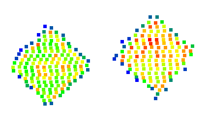
Target-based approaches use specially designed objects to facilitate feature detection and matching. In [3], a checkerboard is used for the calibration of a 2D laser range finder and a camera. Laser points are manually selected and the parameters are estimated using plane-line correspondences. A checkerboard is also utilized in [4], where the segmentation of target point clusters in LiDAR is not discussed. The extraction of checkerboard edges in point cloud is affected by the measurement quantization error, especially at large distances, leading to degraded calibration accuracy [2]. In [2], LiDAR vertices are estimated indirectly by optimizing the transformation between LiDAR and target coordinate frames, where LiDAR targets are detected based on intensities. A good detection performance relies on the target material, target range and the point cloud density, limiting the application scope of the algorithm, as shown in Fig. 1(a). Both [5] and [6] design a rectangular calibration board with four circular holes with different maker patterns. A v-shaped target [7] has also been explored as the calibration target, where extrinsic parameters are estimated via solving the perspective-n-point (PnP) problem. A sphere target has also been leveraged for calibration in [8]. In this paper, square boards are chosen as the calibration target due to their ease of fabrication, enabling easy deployment of the proposed method in real world scenarios.
II-B Appearance based Methods
Image and LiDAR intensity map are used within the mutual information framework for extrinsic calibration [9]. Issues arise when the range sensor does not provide reflectivity information or the observed scene has low reflectivity. In [10], extrinsic parameters are estimated by the optimization of the image intensity variation. This approach assumes constant lighting and suffers from significantly degraded performance in case of illumination variation.
II-C Edge based Methods
LiDAR-camera calibration can be accomplished via registration of LiDAR depth discontinuities and image edges, either using the mutual information framework [11], the grid search method [12] or the optimization method minimizing line projection error [13]. LiDAR edges can be extracted from a single LiDAR scan [12] or from a point cloud map built using LiDAR odometry algorithms [14]. A primary limitation of edge based methods is their assumption that depth discontinuities corresponds mostly to image edges which may be not valid in practice. Moreover, these algorithms require edges in various directions to avoid degenerate optimization.
II-D Learning based Methods
Reg-Net[15] is the pioneering work using deep learning for LiDAR-camera calibration. The techniques in [15] are followed by subsequent works, including the automatic generation of training data by adding perturbation to known calibration, the dual branch architecture for camera and LiDAR feature extraction and the training of several networks for iterative calibration refinement. Lcc-Net[16] is another representative work which uses a cost volume layer for LiDAR-camera feature matching. DXQ-Net [17] learns the calibration flow defined as the offset of the current LiDAR projection in image space. A differentiable optimizer is employed for solving extrinsic parameters. Compared to [16], its generalization ability is greatly enhanced with respect to different environments and sensor installation. However, its accuracy and stability declines noticeably when applied to different sensor models. The generalization issue is common to learning based methods. Besides, the model training requires ground truth calibrations which come from other calibration approaches such as the target-based methods.
III Methodology
III-A System Overview
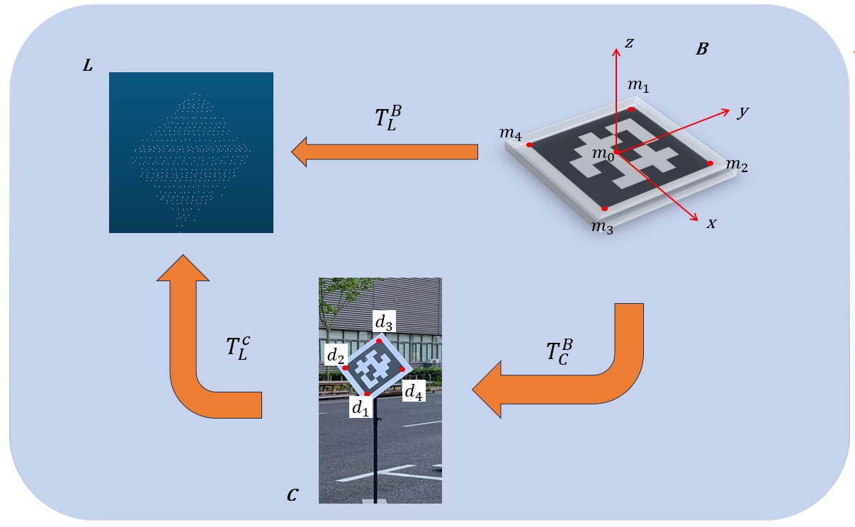
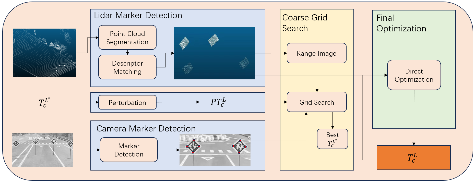
A rigid transformation between two different coordinate systems can be represented by a matrix . As shown in Fig. 2, , , stand for the LiDAR, camera and calibration target (square board) coordinate systems respectively. The right superscript and subscript denote the two coordinate systems involved in the transformation. In our target application scenarios, the coarse extrinsic parameters , camera intrinsic parameters and the square target length are assumed to be known. In particular, the coarse extrinsic parameter can be obtained from vehicle mechanical design. Additionally, the sensors are assumed to be time synchronized. The algorithm begins with calibration target detection from LiDAR and camera. A grid search is then performed to identify the extrinsic candidate which allows the best alignment between LiDAR and camera detection results. At last, a direct optimization method is designed to deliver the final estimation of the extrinsic parameters. Fig. 3 shows the pipeline of the proposed method.
III-B Camera Marker Detection
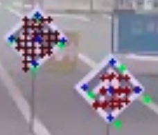
AprilTag[18] is widely used in robotic applications and is chosen for camera target detection in this paper. represents the center and the four vertices of the AprilTag pattern in the target coordinate system , and represents the corners detected in a image. Due to AprilTag’s encoding system, corners detected in the image can establish one-to-one correspondence with the target vertices. The transformation between the camera and a calibration target can then be estimated using the PnP algorithm. Fig. 2 shows an example of the 2D-3D correspondence. For each target, the camera detection algorithm outputs the four image corners and .
III-C LiDAR Marker Detection
This section presents our two-stage algorithm for detecting markers on LiDAR point cloud. Prior to finding potential markers, the point cloud is segmented into several clusters. Then a descriptor representing each cluster is extracted. Considering that only a small portion of clusters contain markers, a descriptor-based verification is adopted to identify board-like, rectangular clusters.
III-C1 Point Cloud Segmentation
As a common first step for point cloud segmentation, ground points are labeled and then removed. Some approaches utilize RANSAC or non-linear optimization to calculate a fine ground plane model, which turn out to be time-consuming. At this point, a fast and robust range image-based method [19] is utilized for segmenting both ground points and non-ground points.
Based on the vertical and horizontal resolutions, each 3D point in the LiDAR sensor’s coordinate system is projected onto a cylindrical range image. Given that the scanning pattern of a MEMS LiDAR might be unevenly distributed, points that locate far in the frustum are removed before calculating the average range of a pixel. Then, with the range image calculated, a four-neighbor breadth-first search for component analysis is conducted pixel-wise[19]. At last, an entire point cloud is segmented into a ground cluster and other non-ground clusters, and the ground cluster is removed.
III-C2 Descriptor Matching
After segmentation, we extract for each non-ground cluster a descriptor which is robust to translation and rotation variance. Existing point cloud descriptor representations mainly fall into two categories: local descriptors and global descriptors. For the sake of computational efficiency and run-time memory cost, global descriptors are considered since they describe the entire object shape and require less computations compared to the local ones. Several types of global descriptors were compared to select the most suitable one for LiDAR board detection, including M2DP[20], Ensemble of Shape Functions (ESF)[21] , Z-projection[22]. M2DP method presents the best performance in terms of precision-recall and time costs for our application.
Before calculating a descriptor, the principal component analysis is performed on each cluster. Then, the points of a cluster are transformed from the sensor’s coordinate system to the eigen space defined by the principal axes and cluster center. In general, M2DP counts the number of point projections in the circular bins of multiple pre-defined planes whose origin aligns with the cluster center. The feature matrix is consisted of multiple rows of projections number vector, and is later decomposed by SVD to form the final descriptor with left and right singular vectors. Different from the original implementation, randomized SVD (rSVD) [23] is employed to accelerate descriptor calculation, which could reduce computational time of matrix decomposition.
| (1) |
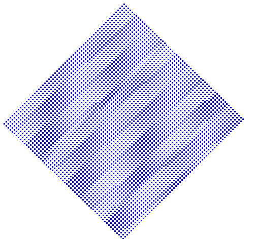
To complete the detection procedure, a descriptor matching method is a must since different observations of a cluster will not be exactly the same. Firstly, as shown in Fig. 1(b), reference descriptors are calculated based on simulated marker board cloud clusters and stored. To compare the similarity between two descriptors, M2DP [20] simply utilizes Euclidean distance (L2 norm) as the similarity measure. Apart from Euclidean distance, other types of similarity measure for descriptor matching are evaluated, including chi-square distance and Pearson’s correlation coefficient (PCC). The latter performs the best regarding robustness and precision-recall. For two n-dimensional vectors and , the Pearson correlation coefficient is defined in the equation1], where and represent mean values and gives an output value ranging from . At last, the negative correlation part is neglected in descriptor matching score, and only the clusters whose matching score exceed the chosen threshold are preserved.
III-D Grid Search
In practice, the translation installation accuracy is of millimeter level. However, it is common to see rotation installation error on the order of one and even a few degrees. Rotation calibration error has a large impact on LiDAR-camera data association, especially for distant objects. Thus a coarse search step is introduced to obtain a more precise initial rotation for the subsequent LiDAR extrinsic optimization.
III-D1 Extrinsic Perturbation
Rotation perturbations are generated by sampling roll, pitch and yaw angles within a predefined range at fixed intervals, and each perturbed angle then is converted to a rotation matrix. Combined with initial extrinsics, a series of extrinsic candidates are generated
III-D2 Extrinsic Candidate Search
With the target pose in camera coordinate system () and an extrinsic candidate in , the board center can be transformed to in LiDAR coordinate system for each target. Throughout the paper, the left superscript indicates the coordinate system that this variable refers to. The quality of the extrinsic candidate is judged based on the total number of LiDAR target points within a fixed-length radius around for all targets. With our experiments showing that the popular k-nearest neighbor(kNN) algorithm is time-consuming with a large number of image-LiDAR frame pairs and several targets in each frame, a novel range image-based search method is proposed to accelerate calculations. First of all, each point from LiDAR marker detections III-C is projected onto a range image based on specified sensor’s resolutions as the reference data structure for searching. Then, the regions for radius search in range image are calculated based on projections of camera marker detection centers. In order to find the region of interest (ROI) in range image for judging alignment, eight vertices of a bounding box whose side length equals the marker board’s length and which is centered at are calculated first. Then, the ROI for each marker detection in range image is defined by the minimum bounding rectangle of these eight vertices’ projections. At last, the number of LiDAR points in ROI is counted pixel-wise, which forms the measure of our judging standard. The best extrinsic candidate has the largest points count number. Alg. 1 shows the implemented search algorithm.
III-E Final Optimization
The coarse grid search step produces initial extrinsic parameters as well as the LiDAR-camera target correspondences. As in [2], for each target, the transformation is first optimized using as the initial value. For each target point cloud cluster , the cost function is defined as below:
| (2) |
| (3) |
| (4) |
Then the target vertices in the LiDAR coordinate system is easily calculated by the transformation of with . After the vertices coordinates of calibration targets in all LiDAR scans are estimated, the final extrinsic can be optimized using the and algorithms. This approach is termed as the indirect optimization method in this paper.
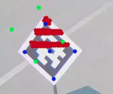
In [2], the parameter in z-axis is tuned according to LiDAR measurement noise, however the effect of different parameter settings is not discussed. If the value is overestimated (larger than real noise level), it will result in insufficient constraints for optimization, thereby leading to inaccurate vertex estimation. Fig. 4(a) shows such an example where the estimated vertex does not agree with the LiDAR point cloud. The parameter tuning will be further discussed in the experimental part.
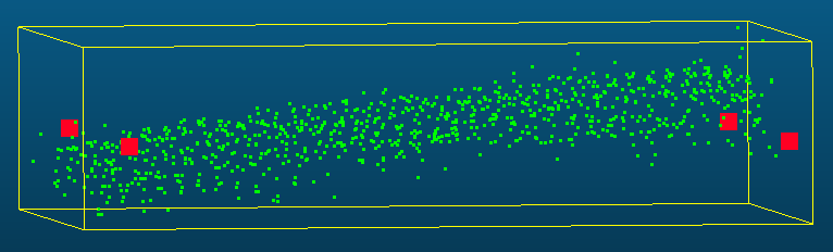
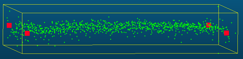
For the indirect optimization method, the accuracy of LiDAR vertex fitting is prone to sparse and sometimes partial LiDAR observation of calibration boards. Fig.5 shows two common scenarios encountered in data acquisition: the calibration targets are either too far or too colse to the sensors. In both cases, the incomplete point cluster can not provide enough constraints to fit precise vertices. Those sub-optimal vertices can adversely affect the precision and robustness of calibration. Inspired by the well-known direct method used in visual odometry [24], a direct optimization method is proposed which still uses the cost in Eq. 2. However, instead of optimizing for each individual LiDAR target, the extrinsic parameters are directly optimized using raw LiDAR board points, avoiding the intermediate vertex fitting step. For direct optimization, these incomplete point clouds combined together are able to give sufficient constraints for extrinsic optimization. Assuming target correspondences in total, the cost can be written as
| (5) |
| (6) |
IV Experiments
The proposed algorithms are tested using real sensory data collected from our vehicle platform. The work of [2] is chosen as the baseline, which is a state of the art method using square targets and is also most related to our work.
IV-A Datasets
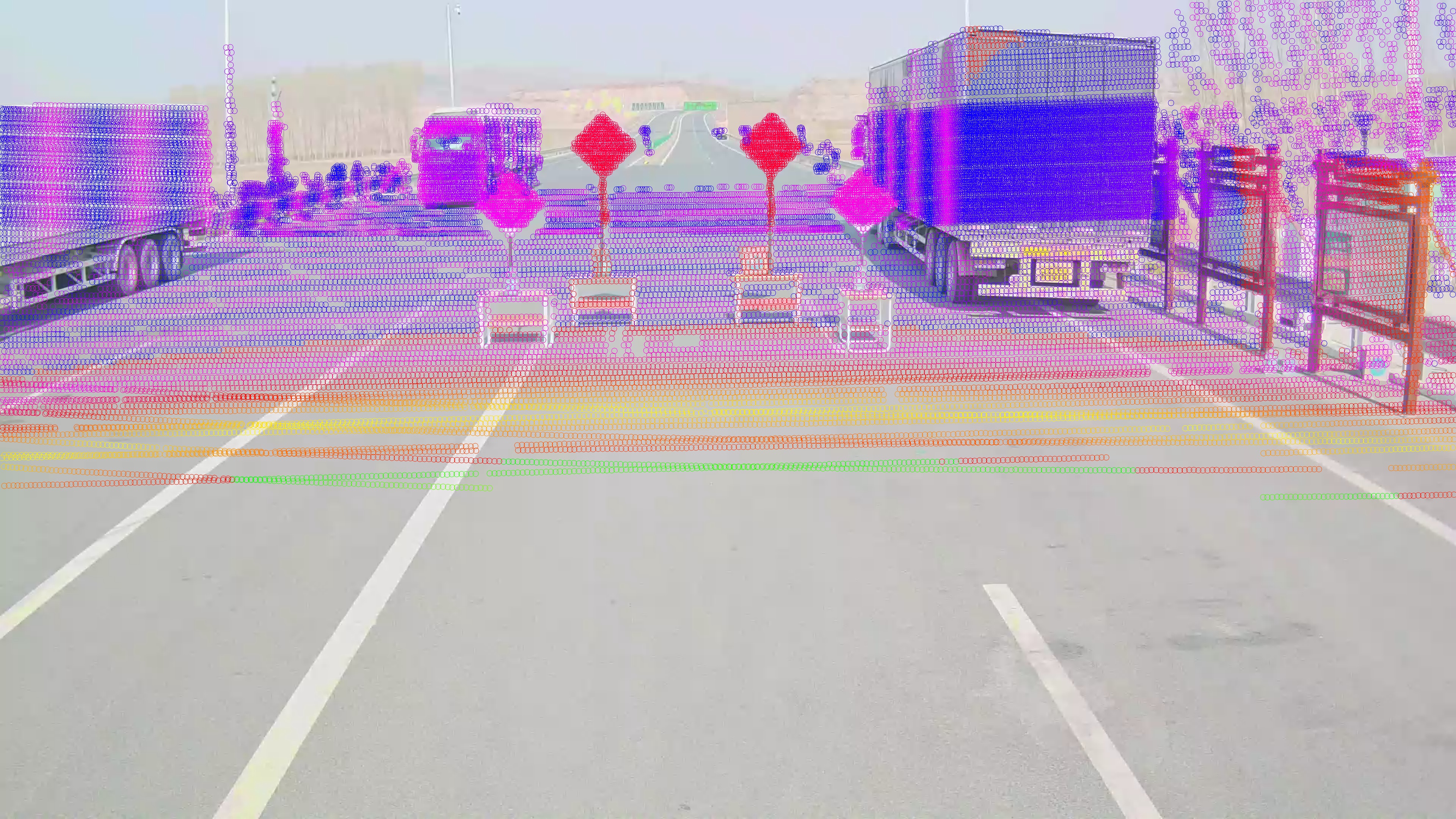
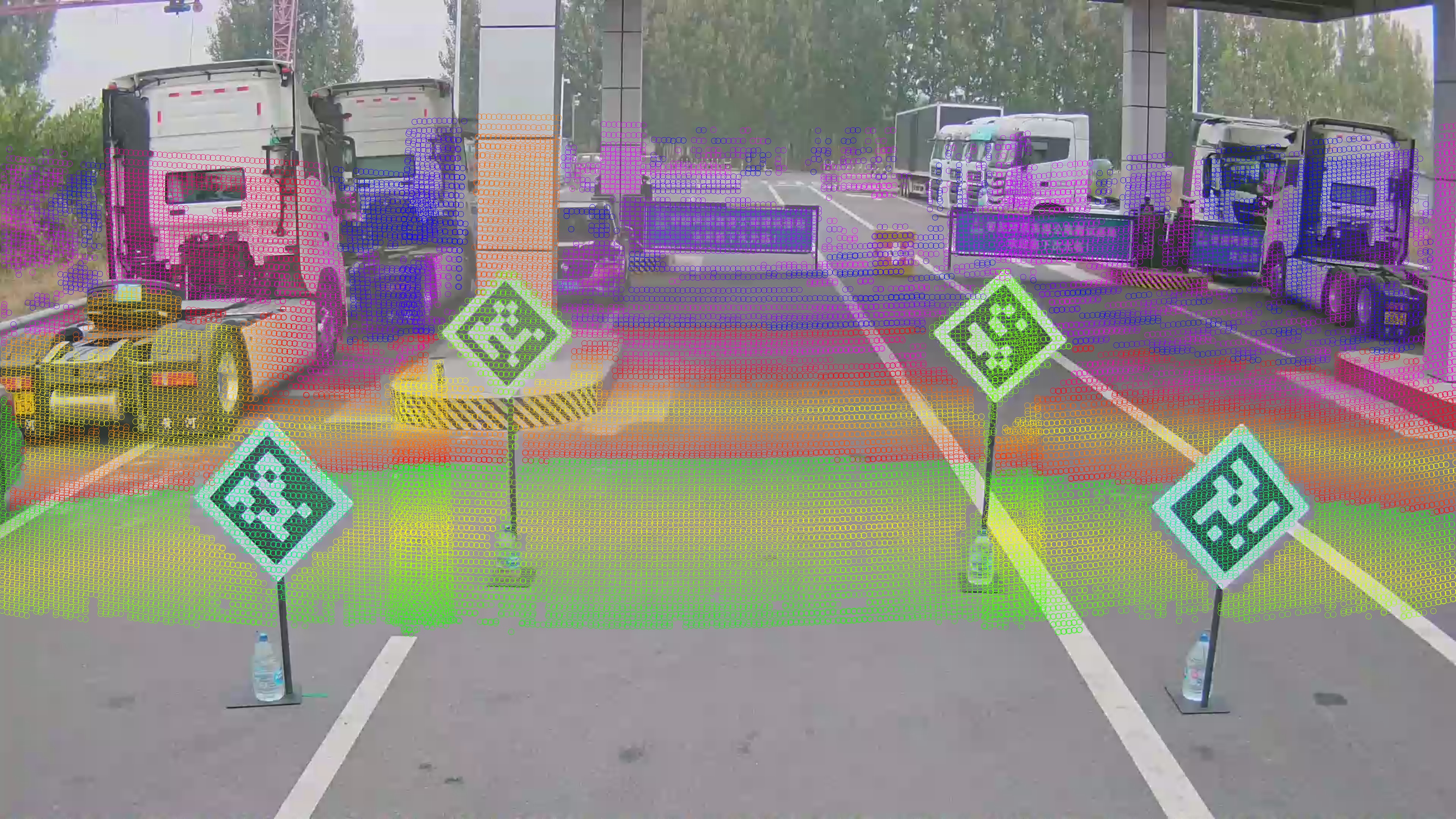
Square calibration boards used in the experiment have a fixed length of 0.6 m and the inner AprilTag marker pattern has a length of 0.48 m. These standard foam boards are mounted on movable stands, with no additional material specifications required. Our camera has a resolution of 3840x1920 pixels. To verify the generalization performance of our proposed algorithms, Robosense111http://robosense.ai/, Innovusion222https://www.seyond.cn/ and Hesai333https://www.hesaitech.com/ are selected for data collection. The vehicle is required to move back and forth within the range of 6 to 30 meters from the calibration targets. Each trajectory lasts around 20 seconds, including 200 LiDAR-camera frame pairs. For each dataset, 5 trajectories are included. Fig. 7 illustrates the data collection scenes.
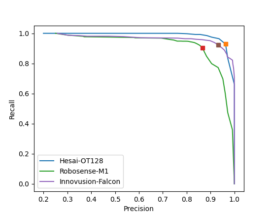
IV-B Evaluation of LiDAR Marker Detection
As III-C presented, we proposed a novel, general and robust LiDAR marker detection algorithm based on geometric descriptor matching without any requirement for board materials. In order to verify the versatility and robustness of the algorithm, the marker centers from different types of LiDAR data in our dataset are annotated. A detection is considered a True Positive (TP) when its center is close to a manually labeled center, otherwise a False Positive (FP). Meanwhile, a labeled center without any detection attached will be regarded as a False Negative(FN). Fig. 6 illustrates curves of different types of LiDAR, including two MEMS LiDAR (Innovusion Falcon, Robosense M1) and one mechanical LiDAR (Hesai OT128), showing that our proposal can adapt to different LiDAR scanning patterns. In this figure, the descriptor matching score threshold for binary classification is set ranging from 0.7 to 0.99, and the threshold used in this paper is 0.94 and same for different types of LiDAR. The square markers in this figure correspond to a score threshold of 0.94.
IV-C Comparison of the Direct and Indirect Optimization Method
The work of [2] did not study the influence of on the calibration accuracy. Table I shows the average projection error (in pixels) between fitted LiDAR vertices and detected camera corners using the indirect optimization method. It is seen that is the best setting. It is also noted that the projection errors of Robosense are larger that the of Innovusion, caused by its larger measurement error compared to Innovusion. Fig. 7 shows an example of projected LiDAR points in the image with the optimized extrinsic parameters.
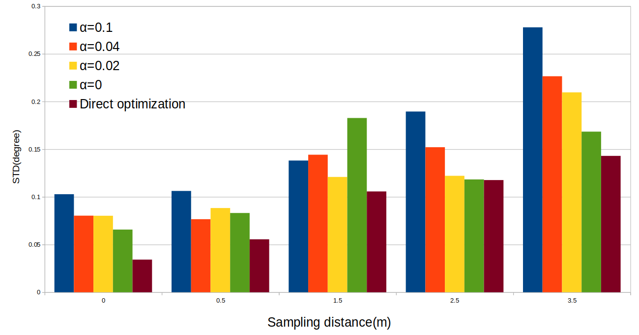
The collected data was down-sampled by distance to compare the robustness of the two optimization methods. That is, a data pair is selected as input for subsequent algorithms only when the vehicle has moved a certain distance. Fig. 8 illustrates the standard derivations (STD) of rotational calibrations. The STD is calculated for 5 different trajectories and the average result (in degree) for roll, pitch and yaw is shown. As the sampling distance increases, the indirect method becomes much more unstable than direct method. Table. II further compares the calibration results of the two optimization methods using data collected at only close or far distances from the calibration targets, shown in Fig.5.
| Parameter | Robosense | Innovusion | Hesai |
|---|---|---|---|
| 9.313 | 5.785 | 8.144 | |
| 7.519 | 4.718 | 6.310 | |
| 7.083 | 4.372 | 5.775 | |
| 6.807 | 4.243 | 5.348 | |
| 6.528 | 4.095 | 5.071 | |
| 6.425 | 4.061 | 5.013 | |
| 6.322 | 4.031 | 5.058 | |
| 6.351 | 3.983 | 4.824 |
IV-D Evaluation of Coarse Grid Search
In order to show the effectiveness of the coarse grid search, a dataset is randomly selected and rotation perturbations are added to the accurately calibrated parameters as the initial value. A rotation perturbation is generated by randomly sampling roll, pitch and yaw angles respectively in the range of -10 to 10 degrees. The search range for our grid search algorithm is from -9 to 9 degrees with the search step being 1.5 degrees. A total of 200 tests are performed, where 100 tests use the proposed grid search to provide initial calibration parameters while the remaining 100 tests directly perform extrinsic optimization. All of the tests using the grid search successfully converged. In contrast, only 6 tests succeed for the 100 tests without using grid search.
IV-E Algorithm Timing
To measure the timing of the algorithm, experiments were performed on a computer equipped with an Intel(R) Core(TM) i7-10750H processor (2.60 GHz, 12 cores) and 32 GB of DDR4 memory. The processing time for 200 image and LiDAR frame pairs is around 18.7 s, 4.93 s, 0.12 s and 1.25 s respectively for LiDAR marker detection, image marker detection, grid search and direct optimization. Note that the indirect optimization algorithm takes 1.63 s. The results demonstrate that the algorithm proposed in this paper is highly efficient and is capable of meeting the real-time requirements of production scenarios.
V Conclusion
A fully automatic approach for LiDAR-camera calibration is proposed in this paper aimed for real world applications in factory manufacturing pipeline and after-sales service. Our method can be applied to different LiDAR sensors, is able to deal with large initial extrinsic errors and achieves superior robustness and accuracy compared to existing algorithms, as demonstrated through experimental evaluations. For future work, the joint calibration of camera intrinsic parameters will be explored within the direct optimization framework.
| Datasets | Close Distance1 | Far Distance2 | ||
|---|---|---|---|---|
| Methods | Indirect | Direct | Indirect | Direct |
| 0.840 | 0.213 | 0.304 | 0.215 | |
| 0.165 | 0.159 | 0.802 | 0.307 | |
| 0.437 | 0.220 | 0.370 | 0.372 | |
-
1
Within 8.5m between targets and sensors
-
2
Above 25m between targets and sensors
References
- [1] M. E. Yecheng Lyu, Lin Bai and X. Huang, “An interactive lidar to camera calibration,” in 2019 IEEE High Performance Extreme Computing Conference (HPEC). IEEE, 2019.
- [2] J.-K. Huang and J. W. Grizzle, “Improvements to target-based 3d lidar to camera calibration,” IEEE Access, vol. 8, pp. 134 101–134 110, 2020.
- [3] Q. Zhang and R. Pless, “Extrinsic calibration of a camera and laser range finder (improves camera calibration),” in 2004 IEEE/RSJ International Conference on Intelligent Robots and Systems (IROS)(IEEE Cat. No. 04CH37566), vol. 3. IEEE, 2004, pp. 2301–2306.
- [4] L. Zhou, Z. Li, and M. Kaess, “Automatic extrinsic calibration of a camera and a 3d lidar using line and plane correspondences,” in 2018 IEEE/RSJ International Conference on Intelligent Robots and Systems (IROS). IEEE, 2018, pp. 5562–5569.
- [5] J. Beltrán, C. Guindel, A. De La Escalera, and F. García, “Automatic extrinsic calibration method for lidar and camera sensor setups,” IEEE Transactions on Intelligent Transportation Systems, vol. 23, no. 10, pp. 17 677–17 689, 2022.
- [6] G. Yan, F. He, C. Shi, P. Wei, X. Cai, and Y. Li, “Joint camera intrinsic and lidar-camera extrinsic calibration,” in 2023 IEEE International Conference on Robotics and Automation (ICRA). IEEE, 2023, pp. 11 446–11 452.
- [7] K. Kwak, D. F. Huber, H. Badino, and T. Kanade, “Extrinsic calibration of a single line scanning lidar and a camera,” in 2011 IEEE/RSJ International Conference on Intelligent Robots and Systems. IEEE, 2011, pp. 3283–3289.
- [8] G.-M. Lee, J.-H. Lee, and S.-Y. Park, “Calibration of vlp-16 lidar and multi-view cameras using a ball for 360 degree 3d color map acquisition,” in 2017 IEEE International Conference on Multisensor Fusion and Integration for Intelligent Systems (MFI). IEEE, 2017, pp. 64–69.
- [9] G. Pandey, J. McBride, S. Savarese, and R. Eustice, “Automatic targetless extrinsic calibration of a 3d lidar and camera by maximizing mutual information,” in Proceedings of the AAAI conference on artificial intelligence, vol. 26, no. 1, 2012, pp. 2053–2059.
- [10] D. Shin, “Computational imaging with small numbers of photons,” Ph.D. dissertation, Massachusetts Institute of Technology, 2016.
- [11] Z. Taylor and J. Nieto, “A mutual information approach to automatic calibration of camera and lidar in natural environments,” in Australian Conference on Robotics and Automation, 2012, pp. 3–5.
- [12] J. Levinson and S. Thrun, “Automatic online calibration of cameras and lasers.” in Robotics: science and systems, vol. 2, no. 7. Citeseer, 2013.
- [13] X. Li, F. He, S. Li, Y. Zhou, C. Xia, and X. Wang, “Accurate and automatic extrinsic calibration for a monocular camera and heterogenous 3d lidars,” IEEE Sensors Journal, vol. 22, no. 16, pp. 16 472–16 480, 2022.
- [14] C. Yuan, X. Liu, X. Hong, and F. Zhang, “Pixel-level extrinsic self calibration of high resolution lidar and camera in targetless environments,” IEEE Robotics and Automation Letters, vol. 6, no. 4, pp. 7517–7524, 2021.
- [15] N. Schneider, F. Piewak, C. Stiller, and U. Franke, “Regnet: Multimodal sensor registration using deep neural networks,” in 2017 IEEE intelligent vehicles symposium (IV). IEEE, 2017, pp. 1803–1810.
- [16] X. Lv, B. Wang, Z. Dou, D. Ye, and S. Wang, “Lccnet: Lidar and camera self-calibration using cost volume network,” in Proceedings of the IEEE/CVF Conference on Computer Vision and Pattern Recognition, 2021, pp. 2894–2901.
- [17] X. Jing, X. Ding, R. Xiong, H. Deng, and W. Yue, “Dxq-net: Differentiable lidar-camera extrinsic calibration using quality-aware flow,” in 2022 IEEE/RSJ International Conference on Intelligent Robots and Systems (IROS). IEEE, 2022, pp. 6235–6241.
- [18] J. Wang and E. Olson, “Apriltag 2: Efficient and robust fiducial detection,” in 2016 IEEE/RSJ International Conference on Intelligent Robots and Systems (IROS). IEEE, 2016, pp. 4193–4198.
- [19] I. Bogoslavskyi and C. Stachniss, “Fast range image-based segmentation of sparse 3d laser scans for online operation,” in 2016 IEEE/RSJ International Conference on Intelligent Robots and Systems (IROS). IEEE, 2016, pp. 163–169.
- [20] L. He, X. Wang, and H. Zhang, “M2dp: A novel 3d point cloud descriptor and its application in loop closure detection,” in 2016 IEEE/RSJ International Conference on Intelligent Robots and Systems (IROS). IEEE, 2016, pp. 231–237.
- [21] W. Wohlkinger and M. Vincze, “Ensemble of shape functions for 3d object classification,” in 2011 IEEE international conference on robotics and biomimetics. IEEE, 2011, pp. 2987–2992.
- [22] N. Muhammad and S. Lacroix, “Loop closure detection using small-sized signatures from 3d lidar data,” in 2011 IEEE International Symposium on Safety, Security, and Rescue Robotics. IEEE, 2011, pp. 333–338.
- [23] X. Feng, W. Yu, and Y. Li, “Faster matrix completion using randomized svd,” in 2018 IEEE 30th International conference on tools with artificial intelligence (ICTAI). IEEE, 2018, pp. 608–615.
- [24] V. K. Jakob Engel and D. Cremers, “Direct sparse odometry,” IEEE Transactions on Pattern Analysis and Machine Intelligence, vol. 40, no. 3, pp. 611–625, 2018.