Incentivized Communication for Federated Bandits
Abstract
Most existing works on federated bandits take it for granted that all clients are altruistic about sharing their data with the server for the collective good whenever needed. Despite their compelling theoretical guarantee on performance and communication efficiency, this assumption is overly idealistic and oftentimes violated in practice, especially when the algorithm is operated over self-interested clients, who are reluctant to share data without explicit benefits. Negligence of such self-interested behaviors can significantly affect the learning efficiency and even the practical operability of federated bandit learning. In light of this, we aim to spark new insights into this under-explored research area by formally introducing an incentivized communication problem for federated bandits, where the server shall motivate clients to share data by providing incentives. Without loss of generality, we instantiate this bandit problem with the contextual linear setting and propose the first incentivized communication protocol, namely, Inc-FedUCB, that achieves near-optimal regret with provable communication and incentive cost guarantees. Extensive empirical experiments on both synthetic and real-world datasets further validate the effectiveness of the proposed method across various environments.
Keywords: Contextual bandit, Federated learning, Incentive Mechanism
1 Introduction
Federated bandit learning has recently emerged as a promising new direction to promote the application of bandit models while preserving privacy by enabling collaboration among multiple distributed clients (Dubey and Pentland, 2020; Wang et al., 2020b; Li and Wang, 2022a; He et al., 2022; Li and Wang, 2022b; Li et al., 2022, 2023; Huang et al., 2021; Tao et al., 2019; Du et al., 2023). The main focus in this line of research is on devising communication-efficient protocols to achieve near-optimal regret in various settings. Most notably, the direction on federated contextual bandits has been actively gaining momentum, since the debut of several benchmark communication protocols for contextual linear bandits in the P2P (Korda et al., 2016) and star-shaped (Wang et al., 2020b) networks. Many subsequent studies have explored diverse configurations of the clients’ and environmental modeling factors and addressed new challenges arising in these contexts. Notable recent advancements include extensions to asynchronous linear bandits (Li and Wang, 2022a; He et al., 2022), generalized liner bandits (Li and Wang, 2022b), and kernelized contextual bandits (Li et al., 2022, 2023).
Despite the extensive exploration of various settings, almost all existing federated bandit algorithms rely on the assumption that every client in the system is willing to share their local data/model with the server, regardless of the communication protocol design. For instance, synchronous protocols (Wang et al., 2020b; Li and Wang, 2022b) require all clients to simultaneously engage in data exchange with the server in every communication round. Similarly, asynchronous protocols (Li and Wang, 2022a; Li et al., 2023; He et al., 2022) also assume clients must participate in communication as long as the individualized upload or download event is triggered, albeit allowing interruptions by external factors (e.g., network failure).
In contrast, our work is motivated by the practical observation that many clients in a federated system are inherently self-interested and thus reluctant to share data without receiving explicit benefits from the server (Karimireddy et al., 2022). For instance, consider the following scenario: a recommendation platform (server) wants its mobile app users (clients) to opt in its new recommendation service, which switches previous on-device local bandit algorithm to a federated bandit algorithm. Although the new service is expected to improve the overall recommendation quality for all clients, particular clients may not be willing to participate in this collaborative learning, as the expected gain for them might not compensate their locally increased cost (e.g., communication bandwidth, added computation, lost control of their data, and etc). In this case, additional actions have to be taken by the server to encourage participation, as it has no power to force clients. This exemplifies the most critical concern in the real-world application of federated learning (Karimireddy et al., 2022). And a typical solution is known as incentive mechanism, which motivates individuals to contribute to the social welfare goal by offering incentives such as monetary compensation.
While recent studies have explored incentivized data sharing in federated learning (Pei, 2020; Tu et al., 2022), most of which only focused on the supervised offline learning setting (Karimireddy et al., 2022). To our best knowledge, ours is the first work that studies incentive design for federated bandit learning, which inherently imposes new challenges. First, there is a lack of well-defined metric to measure the utility of data sharing, which rationalizes a client’s participation. Under the context of bandit learning, we measure data utility by the expected regret reduction from the exchanged data for each client. As a result, each client values data (e.g., sufficient statistics) from the server differently, depending on how such data aligns with their local data (e.g., the more similar the less valuable). Second, the server is set to minimize regret across all clients through data exchange. But as the server does not generate data, it can be easily trapped by the situation where its collected data cannot pass the critical mass to ensure every participating client’s regret is close to optimal (e.g., the data under server’s possession cannot motivate the clients who have more valuable data to participate). To break the deadlock, we equip the server to provide monetary incentives. Subsequently, the server needs to minimize its cumulative monetary payments, in addition to the regret and communication minimization objectives as required by federated bandit learning. We propose a provably effective incentivized communication protocol, based on a heuristic search strategy to balance these distinct learning objectives. Our solution obtains near-optimal regret with provable communication and incentive cost guarantees. Extensive empirical simulations on both synthetic and real-world datasets further demonstrate the effectiveness of the proposed protocol in various federated bandit learning environments.
2 Related Work
Federated Bandit Learning
One important branch in this area is federated multi-armed bandits (MABs), which has been well-studied in the literature (Liu and Zhao, 2010; Szorenyi et al., 2013; Landgren et al., 2016; Chakraborty et al., 2017; Landgren et al., 2018; Martínez-Rubio et al., 2019; Sankararaman et al., 2019; Wang et al., 2020a; Shi et al., 2020, 2021; Zhu et al., 2021). The other line of work focuses on the federated contextual bandit setting (Korda et al., 2016; Wang et al., 2020b), which has recently attracted increasing attention. Wang et al. (2020b) and Korda et al. (2016) are among the first to investigate this problem, where multiple communication protocols for linear bandits (Abbasi-Yadkori et al., 2011; Li et al., 2010) in star-shaped and P2P networks are proposed. Many follow-up works on federated linear bandits (Dubey and Pentland, 2020; Huang et al., 2021; Li and Wang, 2022a; He et al., 2022) have emerged with different client and environment settings, such as investigating fixed arm set (Huang et al., 2021), incorporating differential privacy (Dubey and Pentland, 2020), and introducing asynchronous communication (He et al., 2022; Li and Wang, 2022a). Li and Wang (2022b) extend the federated linear bandits to generalized linear bandits (Filippi et al., 2010). And they further investigated federated learning for kernelized contextual bandits in both synchronous and asynchronous settings (Li et al., 2022, 2023).
In this work, we situate the incentivized federated bandit learning problem under linear bandits with time-varying arm sets, which is a popular setting in many recent works (Wang et al., 2020b; Dubey and Pentland, 2020; Li and Wang, 2022a; He et al., 2022). But we do not assume the clients will always participate in data sharing: they will choose not to share its data with the server if the resulting benefit of data sharing is not deemed to outweigh the cost. Here we need to differentiate our setting from those with asynchronous communication, e.g., Asyn-LinUCB (Li and Wang, 2022a). Such algorithms still assume all clients are willing to share, though sometimes the communication can be interrupted by some external factors (e.g., network failure). We do not assume communication failures and leave it as our future work. Instead, we assume the clients need to be motivated to participate in federated learning, and our focus is to devise the minimum incentives to obtain the desired regret and communication cost for all participating clients.
Incentivized Federated Learning
Data sharing is essential to the success of federated learning (Pei, 2020), where client participation plays a crucial role. However, participation involves costs, such as the need for additional computing and communication resources, and the risk of potential privacy breaches, which can lead to opt-outs (Cho et al., 2022; Hu and Gong, 2020). In light of this, recent research has focused on investigating incentive mechanisms that motivate clients to contribute, rather than assuming their willingness to participate. Most of the existing research involves multiple decentralized clients solving the same task, typically with different copies of IID datasets, where the focus is on designing data valuation methods that ensure fairness or achieve a specific accuracy objective (Sim et al., 2020; Xu et al., 2021; Donahue and Kleinberg, 2023). On the other hand, Donahue and Kleinberg (2021) study voluntary participation in model-sharing games, where clients may opt out due to biased global models caused by the aggregated non-IID datasets. More recently, Karimireddy et al. (2022) investigated incentive mechanism design for data maximization while avoiding free riders. For a detailed discussion of this topic, we refer readers to recent surveys on incentive mechanism design in federated learning (Zhan et al., 2021; Tu et al., 2022).
However, most works on incentivized federated learning only focus on better model estimation among fixed offline datasets, which does not apply to the bandit learning problem, where the exploration of growing data is also part of the objective. More importantly, in our incentivized federated bandit problem, the server is obligated to improve the overall performance of the learning system, i.e., minimizing regret among all clients, which is essentially different from previous studies where the server only selectively incentivizes clients to achieve a certain accuracy (Sim et al., 2020) or to investigate how much accuracy the system can achieve without payment (Karimireddy et al., 2022).
3 Preliminaries
In this section, we formally introduce the incentivized communication problem for federated bandits under the contextual linear bandit setting.
3.1 Federated Bandit Learning
We consider a learning system consisting of (1) clients that directly interact with the environment by taking actions and receiving the corresponding rewards, and (2) a central server that coordinates the communication among the clients to facilitate their learning collectively. The clients can only communicate with the central server, but not with each other, resulting in a star-shaped communication network. At each time step , an arbitrary client becomes active and chooses an arm from a candidate set , and then receives the corresponding reward feedback . Note that is time-varying, denotes the unknown reward function shared by all clients, and denotes zero mean sub-Gaussian noise with known variance .
The performance of the learning system is measured by the cumulative (pseudo) regret over all clients in the finite time horizon , i.e., , where is the regret incurred by client at time step . Moreover, under the federated learning setting, the system also needs to keep the communication cost low, which is measured by the total number of scalars (Wang et al., 2020b) being transferred across the system up to time .
With the linear reward assumption, i.e., , where denotes the unknown parameter, a ridge regression estimator can be constructed based on sufficient statistics from all clients at each time step , where and (Lattimore and Szepesvári, 2020). Using under the Optimism in the Face of Uncertainty (OFUL) principle (Abbasi-Yadkori et al., 2011), one can obtain the optimal regret . To achieve this regret bound in the federated setting, a naive method is to immediately share statistics of each newly collected data sample to all other clients in the system, which essentially recovers its centralized counterpart. However, this solution incurs a disastrous communication cost . On the other extreme, if no communication occurs throughout the entire time horizon (i.e., ), the regret upper bound can be up to when each client interacts with the environment at the same frequency, indicating the importance of timely data/model aggregation in reducing .
To balance this trade-off between regret and communication cost, prior research efforts centered around designing communication-efficient protocols for federated bandits that feature the “delayed update” of sufficient statistics (Wang et al., 2020b; Li and Wang, 2022a; He et al., 2022). Specifically, each client only has a delayed copy of and , denoted as , where is the aggregated sufficient statistics shared by the server in the last communication, and is the accumulated local updates that client obtain from its interactions with the environment since . In essence, the success of these algorithms lies in the fact that typically changes slowly and thus has little instant impact on the regret for most time steps. Therefore, existing protocols that only require occasional communications can still achieve nearly optimal regret, despite the limitation on assuming clients’ willingness on participation as we discussed before.
3.2 Incentivized Federated Bandits
Different from the prior works in this line of research, where all clients altruistically share their data with the server whenever a communication round is triggered, we are intrigued in a more realistic setting where clients are self-interested and thus reluctant to share data with the server if not well motivated. Formally, each client in the federated system inherently experiences a cost 111Note that if the costs are trivially set to zero, then clients have no reason to opt-out of data sharing and our problem essentially reduces to the standard federated bandits problem (Wang et al., 2020b). of data sharing, denoted by , due to their individual consumption of computing resources in local updates or concerns about potential privacy breaches caused by communication with the server. Moreover, as the client has nothing to lose when there is no local update to share in a communication round at time step , in this case we assume the cost is 0, i.e., . As a result, the server needs to motivate clients to participate in data sharing via the incentive mechanism , which takes as inputs a collection of client local updates and a vector of cost values , and outputs the incentive to be distributed among the clients. Specifically, to make it possible to measure gains and losses of utility in terms of real-valued incentives (e.g., monetary payment), we adopt the standard quasi-linear utility function assumption, as is standard in economic analysis (Allais, 1953; Pemberton and Rau, 2007).
At each communication round, a client decides whether to share its local update with the server based on the potential utility gained from participation, i.e., the difference between the incentive and the cost of data sharing. This requires the incentive mechanism to be individually rational:
Definition 1 (Individual Rationality (Myerson and Satterthwaite, 1983))
An incentive mechanism is individually rational if for any in the participant set at time step , we have
| (1) |
In other words, each participant must be guaranteed non-negative utility by participating in data sharing under .
The server coordinates with all clients and incentivizes them to participate in the communication to realize its own objective (e.g., collective regret minimization). This requires to be sufficient:
Definition 2 (Sufficiency)
An incentive mechanism is sufficient if the resulting outcome satisfies the server’s objective.
Typically, under different application scenarios, the server may have different objectives, such as regret minimization or best arm identification. In this work, we set the objective of the server to minimize the regret across all clients; and ideally the server aims to attain the optimal regret in the centralized setting via the incentivized communication. Therefore, we consider an incentive mechanism is sufficient if it ensures that the resulting accumulated regret is bounded by .
4 Methodology
The communication backbone of our solution derives from DisLinUCB (Wang et al., 2020b), which is a widely adopted paradigm for federated linear bandits. We adopt their strategy for arm selection and communication trigger, so as to focus on the incentive mechanism design. We name the resulting algorithm Inc-FedUCB, and present it in Algorithm 1. Note that the two incentive mechanisms to be presented in Section 4.2 and 4.3 are not specific to any federated bandit learning algorithms, and each of them can be easily extended to alternative workarounds as a plug-in to accommodate the incentivized federated learning setting. For clarity, a summary of technical notations can be found in Table 7.
4.1 A General Framework: Inc-FedUCB Algorithm
Our framework comprises three main steps: 1) client’s local update; 2) communication trigger; and 3) incentivized data exchange among the server and clients. Specifically, after initialization, an active client performs a local update in each time step and checks the communication trigger. If a communication round is triggered, the system performs incentivized data exchange between clients and the server. Otherwise, no communication is needed.
Formally, at each time step , an arbitrary client becomes active and interacts with its environment using observed arm set (Line 5). Specifically, it selects an arm that maximizes the UCB score as follows (Line 6):
| (2) |
where is the ridge regression estimator of with regularization parameter , , and . denotes the covariance matrix constructed using data available to client up to time . After obtaining a new data point from the environment, client checks the communication event trigger (Line 9), where denotes the time elapsed since the last time it communicated with the server and denotes the specified threshold.
Incentivized Data Exchange
With the above event trigger, communication rounds only occur if (1) a substantial amount of new data has been accumulated locally at client , and/or (2) significant time has elapsed since the last communication. However, in our incentivized setting, triggering a communication round does not necessarily lead to data exchange at time step , as the participant set may be empty (Line 11). This characterizes the fundamental difference between Inc-FedUCB and DisLinUCB (Wang et al., 2020b): we no longer assume all clients will share their data with the server in an altruistic manner; instead, a rational client only shares its local update with the server if the condition in Eq. (1) is met. In light of this, to evaluate the potential benefit of data sharing, all clients must first reveal the value of their data to the server before the server determines the incentive. Hence, after a communication round is triggered, all clients upload their latest sufficient statistics update to the server (Line 10) to facilitate data valuation and participant selection in the incentive mechanism (Line 11). Note that this disclosure does not compromise clients’ privacy, as the clients’ secret lies in that is constructed by the rewards. Only participating clients will upload their to the server (Line 13). After collecting data from all participants, the server downloads the aggregated updates and to every client (Line 17-20). Following the convention in federated bandit learning (Wang et al., 2020b), the communication cost is defined as the total number of scalars transferred during this data exchange process.
4.2 Payment-free Incentive Mechanism
As mentioned in Section 1, in federated bandit learning, clients can reduce their regret by using models constructed via shared data. Denote as the covariance matrix constructed by all available data in the system at time step . Based on Lemma 5 and 7, the instantaneous regret of client is upper bounded by:
| (3) |
where the determinant ratio reflects the additional regret due to the delayed synchronization between client ’s local sufficient statistics and the global optimal oracle. Therefore, minimizing this ratio directly corresponds to reducing client ’s regret. For example, full communication keeps the ratio at 1, which recovers the regret of the centralized setting discussed in Section 3.1.
Therefore, given the client’s desire for regret minimization, the data itself can be used as a form of incentive by the server. And the star-shaped communication network also gives the server an information advantage over any single client in the system: a client can only communicate with the server, while the server can communicate with every client. Therefore, the server should utilize this advantage to create incentives (i.e., the LHS of Eq. (1)), and a natural design to evaluate this data incentive is:
| (4) |
where denotes the data that the server can offer to client during the communication at time (i.e., current local updates from other participants that have not been shared with the server) and is the historically aggregated updates stored in the server that has not been shared with client . Eq. (4) suggests a substantial increase in the determinant of the client’s local data is desired by the client, which results in regret reduction.
With the above data valuation in Eq. (4), we propose the payment-free incentive mechanism that motivates clients to share data by redistributing data collected from participating clients. We present this mechanism in Algorithm 2, and briefly sketch it below. First, we initiate the participant set , assuming all clients agree to participate. Then, we iteratively update by checking the willingness of each client in according to Eq. (1). If is empty or all clients in it are participating, then terminate; otherwise, remove client from and repeat the process.
While this payment-free incentive mechanism is neat and intuitive, it has no guarantee on the amount of data that can be collected. To see this, we provide a theoretical negative result with rigorous regret analysis in Theorem 3 (see proof in Appendix C).
Theorem 3 (Sub-optimal Regret)
When there are at most number of clients (for some constant ), whose cost value , there exists a linear bandit instance with such that for , the expected regret for Inc-FedUCB algorithm with payment-free incentive mechanism is at least .
Recall the discussion in Section 3.1, when there is no communication is upper bounded by . Hence, in the worst-case scenario, the payment-free incentive mechanism might not motivate any client to participate. It is thus not a sufficient mechanism.
4.3 Payment-efficient Incentive Mechanism
To address the insufficiency issue, we further devise a payment-efficient incentive mechanism that introduces additional monetary incentives to motivate clients’ participation:
| (5) |
where is the data incentive defined in Eq. (4), and is the real-valued monetary incentive, i.e., the payment assigned to client for its participation. Specifically, we are intrigued by the question: rather than trivially paying unlimited amounts to ensure everyone’s participation, can we devise an incentive mechanism that guarantees a certain level of client participation such that the overall regret is still nearly optimal but under acceptable monetary incentive cost?
Inspired by the determinant ratio principle discussed in Eq. (3), we propose to control the overall regret by ensuring that every client closely approximates the oracle after each communication round, which can be formalized as , where is to be shared with all clients and . The parameter characterizes the chosen gap between the practical and optimal regrets that the server commits to. Denote the set of clients motivated by at time as and those motivated by as , and thus . At each communication round, the server needs to find the minimum such that pooling local updates from satisfies the required regret reduction for the entire system.
| (6) |
Algorithm 2 maximizes , and thus the servers should compute on top of optimal and resulting , which however is still combinatorially hard. First, a brute-force search can yield a time complexity up to . Second, different from typical optimal subset selection problems (Kohavi and John, 1997), the dynamic interplay among clients in our specific context brings a unique challenge: once a client is incentivized to share data, the other uninvolved clients may change their willingness due to the increased data incentive, making the problem even more intricate.
To solve the above problem, we propose a heuristic ranking-based method, as outlined in Algorithm 3. The heuristic is to rank clients by the marginal gain they bring to the server’s determinant, as formally defined in Eq. (6), which helps minimize the number of clients requiring monetary incentives, while empowering the participation of other clients motivated by the aggregated data. This forms an iterative search process: First, we rank all non-participating clients (Line 2-3) by their potential contribution to the server (with participant set committed); Then, we segment the list by , anyone whose participation satisfies the overall gap constraint is an immediately valid choice (Line 4). The first client in the valid list and its payment ( if not available) will be our last resort (Line 5); Lastly, we check if there exist potentially more favorable solutions from the invalid list (Line 6). Specifically, we try to elicit up to ( if is not available) clients from the invalid list in rounds, where only one client will be chosen using the same heuristic in each round. If having clients from the invalid list also satisfies the constraint and results in a reduced monetary incentive cost compared to , then we opt for this alternative solution. Otherwise, we will adhere to the last resort.
This Heuristic Search is detailed in Appendix A, and it demonstrates a time complexity of only in the worst-case scenarios, i.e., . Theorem 4 guarantees the sufficiency of this mechanism w.r.t communication and payment bounds.
Theorem 4
Under threshold and clients’ committed data sharing cost , with high probability the monetary incentive cost of Inc-FedUCB satisfies
where is the number of epochs client gets paid throughout time horizon , is the total number of epochs, which is bounded by setting communication threshold , where .
Henceforth, the communication cost satisfies
Furthermore, by setting , the cumulative regret is
5 Experiments
We simulate the incentivized federated bandit problem under various environment settings. Specifically, we create an environment of clients with cost of data sharing , total number of iterations , feature dimension , and time-varing arm pool size . By default, we set . Due to the space limit, more detailed results and discussions on real-world dataset can be found in Appendix E.
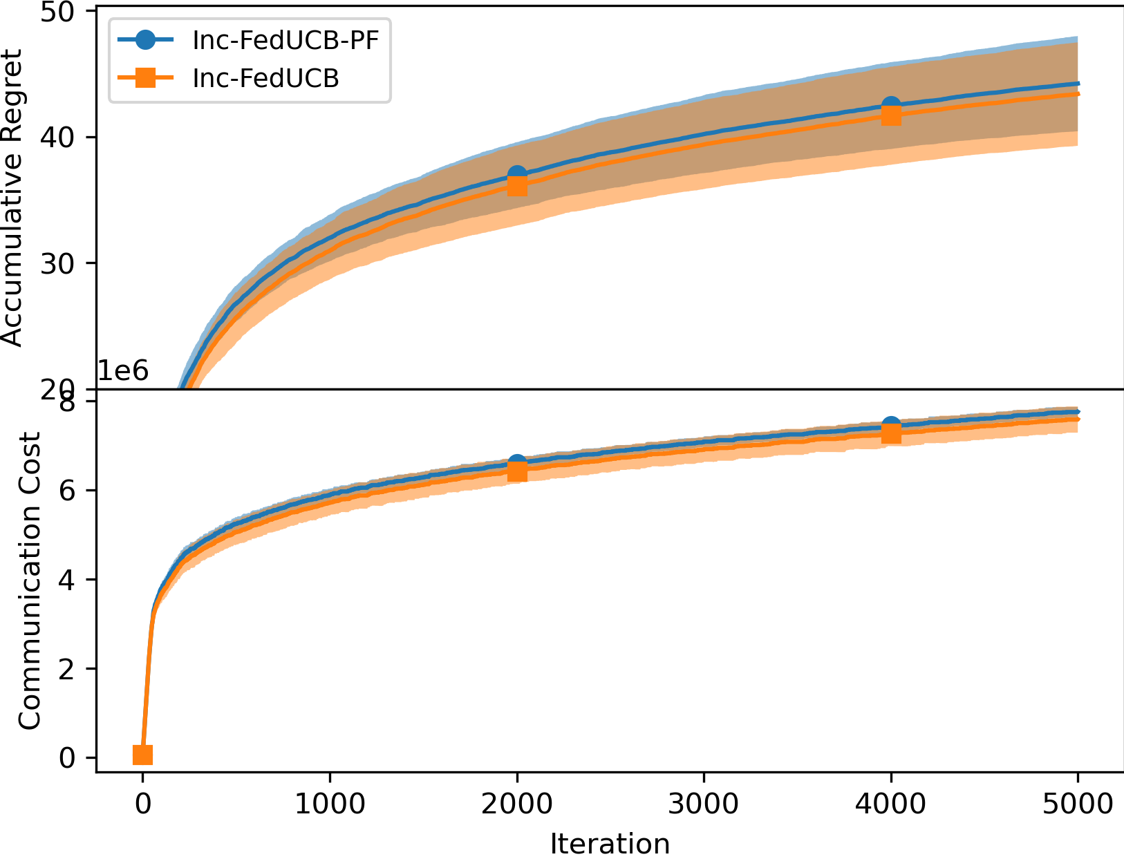
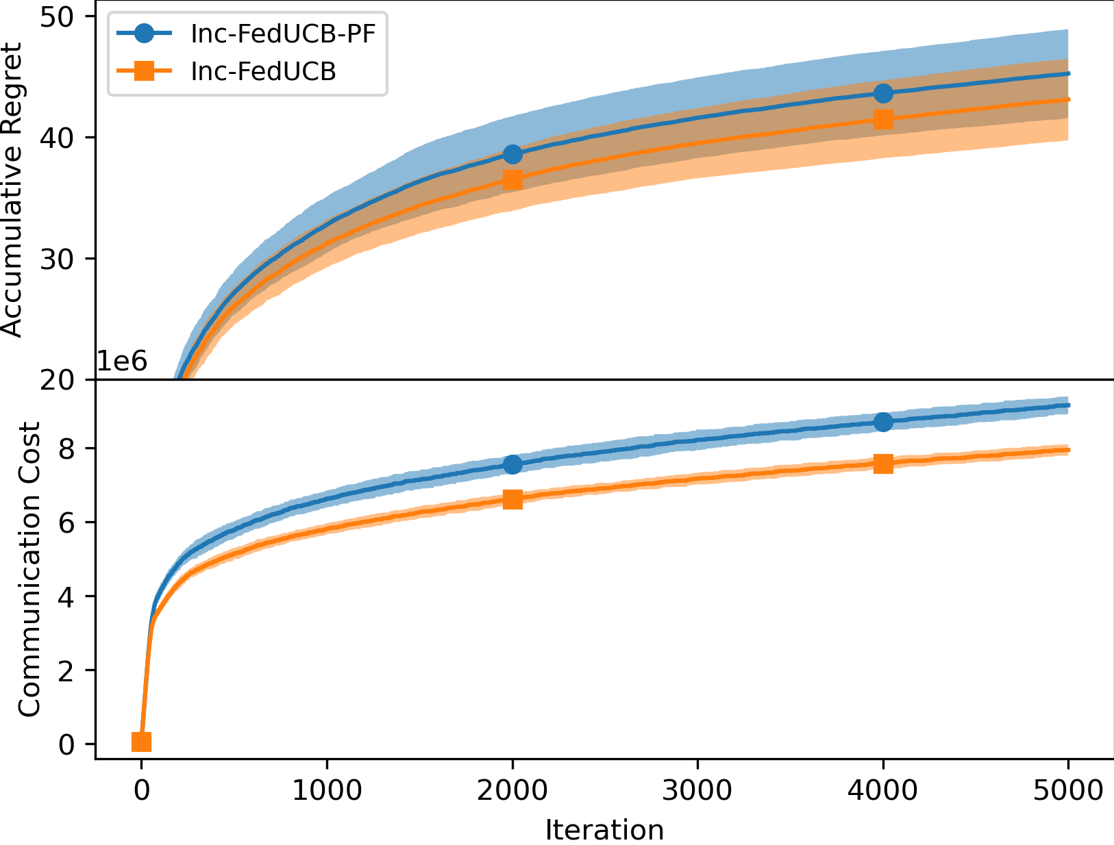
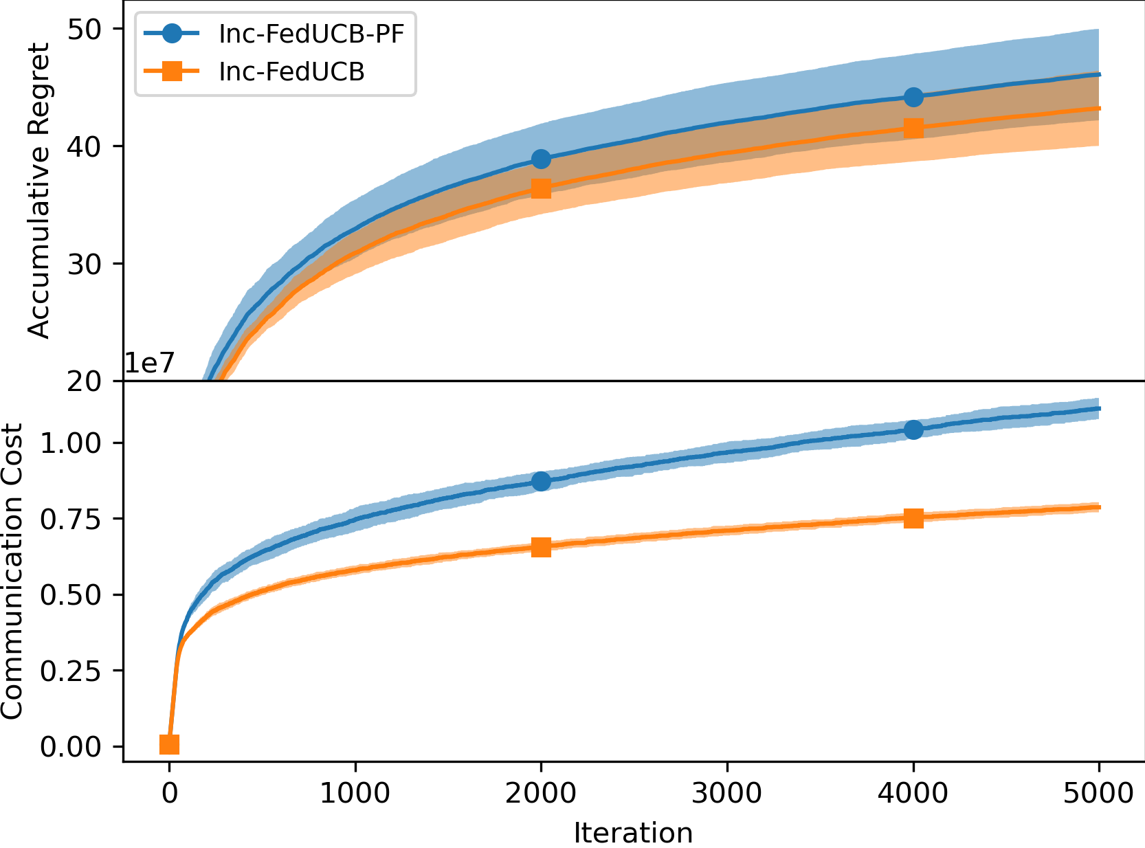
5.1 Payment-free vs. Payment-efficient
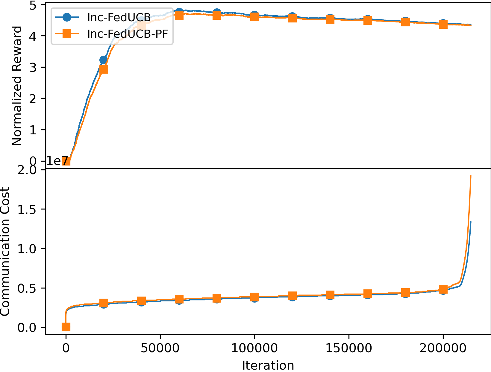
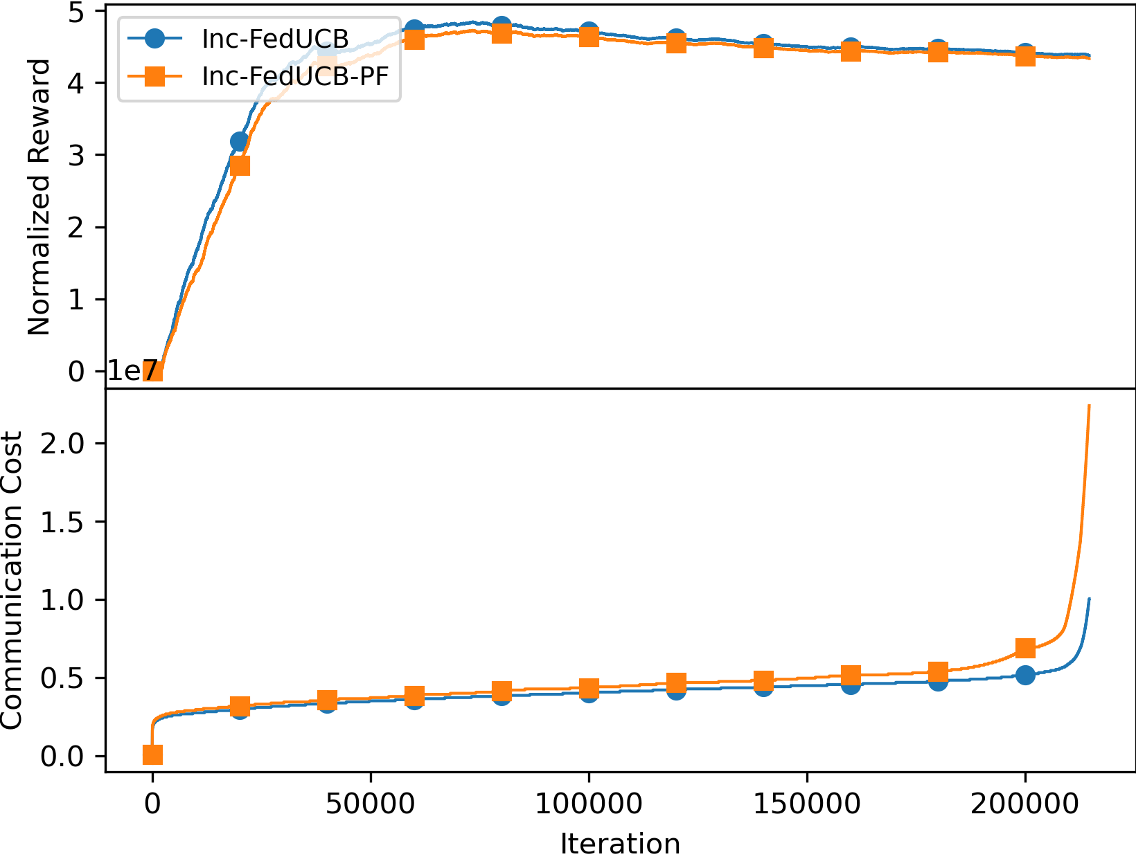
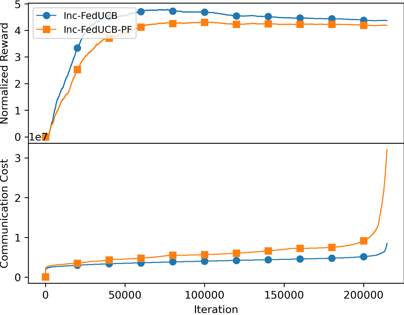
We first empirically compared the performance of the payment-free mechanism (named as Inc-FedUCB-PF) and the payment-efficient mechanism Inc-FedUCB in Figure 1. It is clear that the added monetary incentives lead to lower regret and communication costs, particularly with increased . Lower regret is expected as more data can be collected and shared; while the reduced communication cost is contributed by reduced communication frequency. When less clients can be motivated in one communication round, more communication rounds will be triggered as the clients tend to have outdated local statistics.
5.2 Ablation Study on Heuristic Search
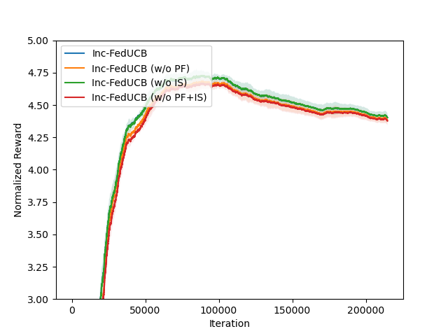
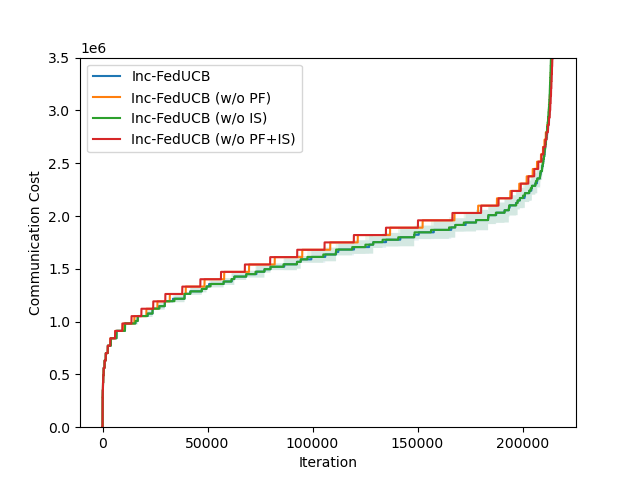
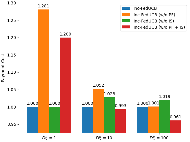
To investigate the impact of different components in our heuristic search, we compare the full-fledged model Inc-FedUCB with following variants on various environments: (1) Inc-FedUCB (w/o PF): without payment-free incentive mechanism, where the server only use money to incentivize clients; (2) Inc-FedUCB (w/o IS): without iterative search, where the server only rank the clients once. (3) Inc-FedUCB (w/o PF + IS): without both above strategies.
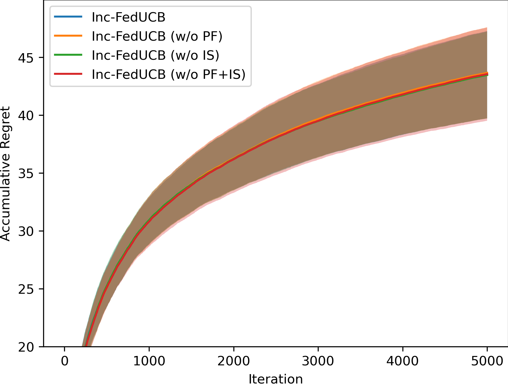
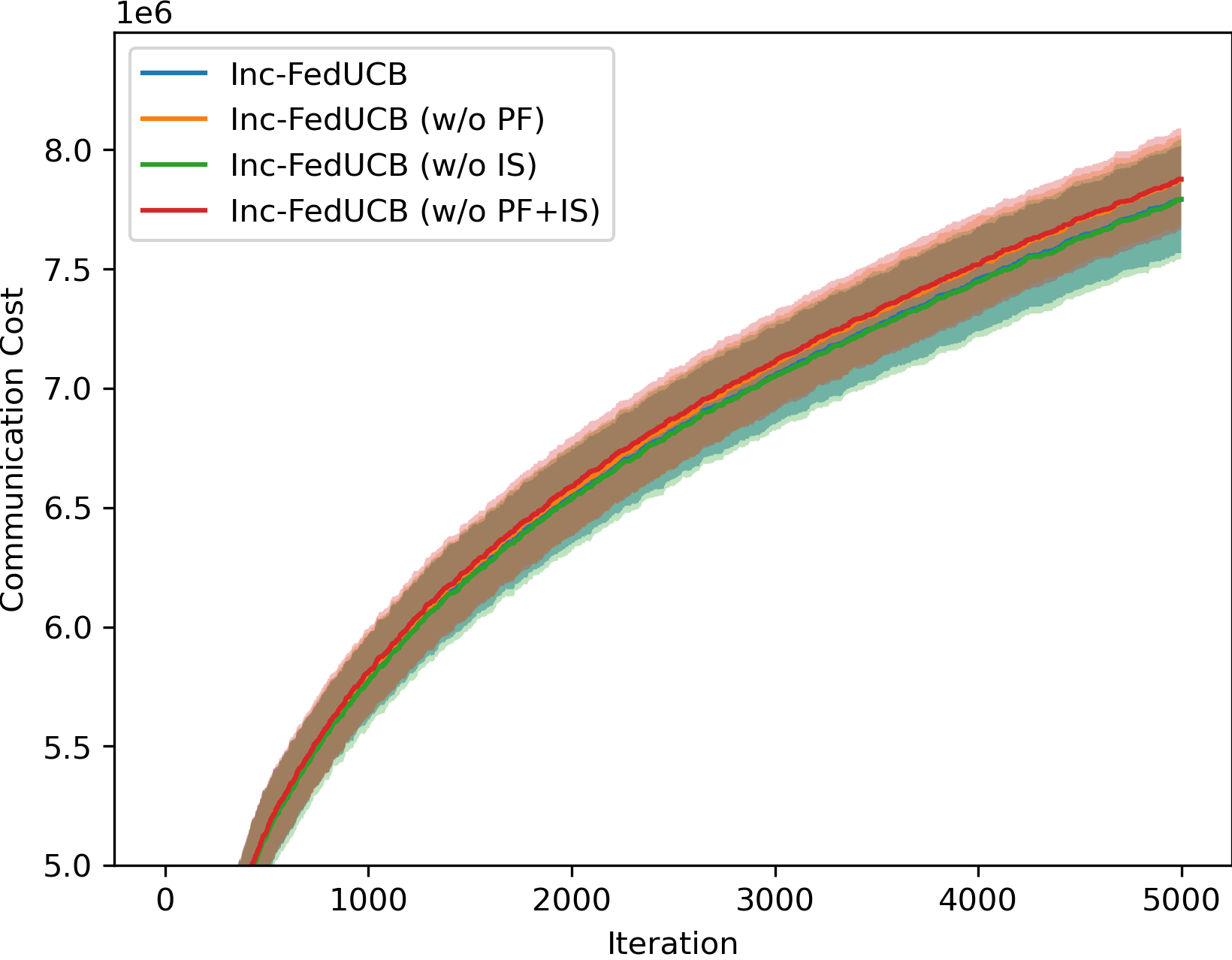
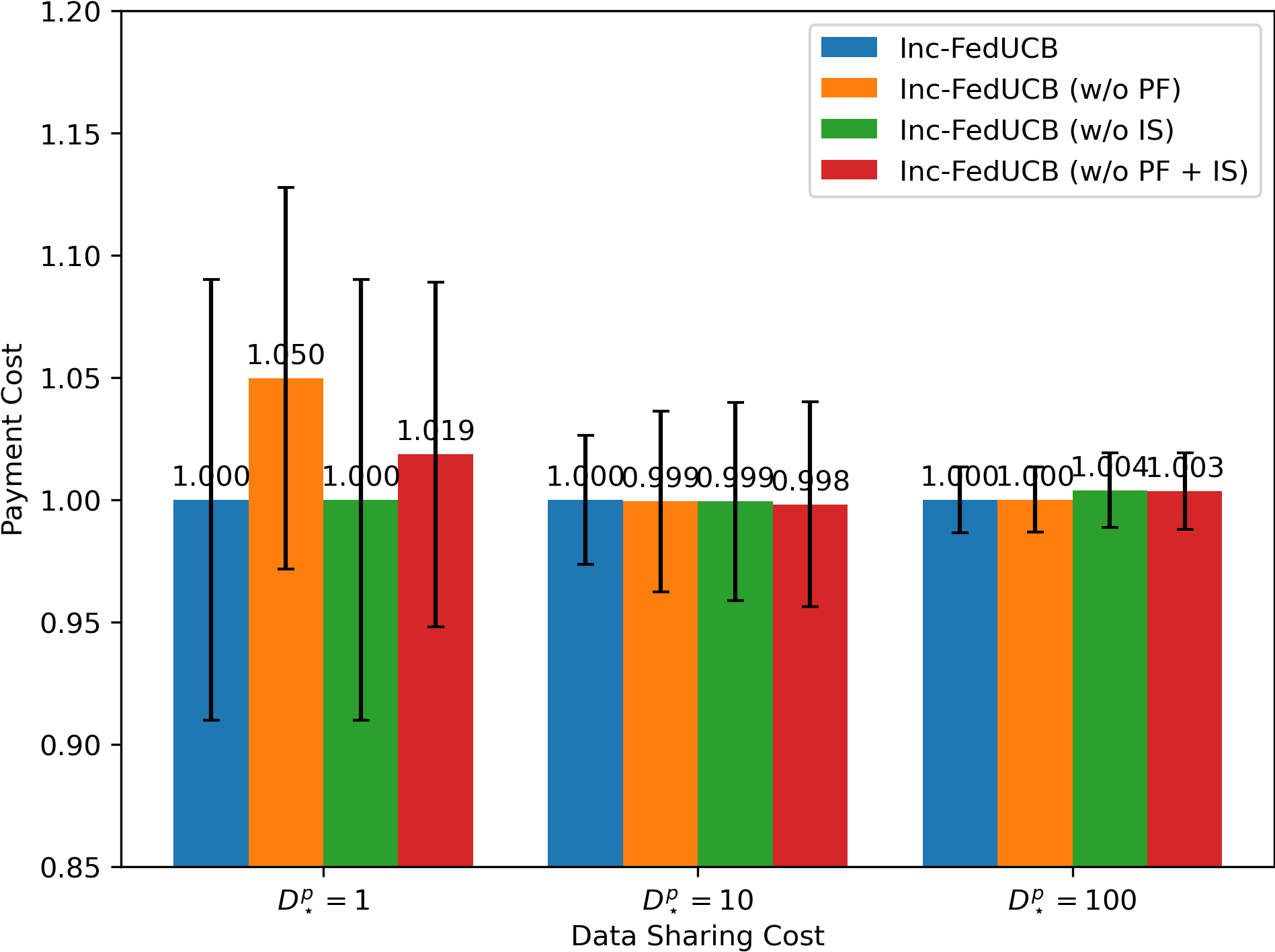
In Figure 2, we present the averaged learning trajectories of regret and communication cost, along with the final payment costs (normalized) under different . The results indicate that the full-fledged Inc-FedUCB consistently outperforms all other variants in various environments. Additionally, there is a substantial gap between the variants with and without the PF strategy, emphasizing the significance of leveraging server’s information advantage to motivate participation.
5.3 Environment & Hyper-Parameter Study
We further explored diverse hyperparameter settings for Inc-FedUCB in various environments with varying , along with the comparison with DisLinUCB (Wang et al., 2020b) (only comparable when ).
| DisLinUCB | Inc-FedUCB () | Inc-FedUCB () | Inc-FedUCB () | ||
| Regret (Acc.) | 48.46 | 48.46 | 48.46 () | 48.46 () | |
| Commu. Cost | 7,605,000 | 7,605,000 | 7,605,000 () | 7,605,000 () | |
| Pay. Cost | \ | 0 | 0 () | 0 () | |
| Regret (Acc.) | \ | 48.46 | 47.70 () | 48.38 () | |
| Commu. Cost | \ | 7,605,000 | 7,668,825 () | 7,733,575 () | |
| Pay. Cost | \ | 75.12 | 60.94 () | 22.34 () | |
| Regret (Acc.) | \ | 48.46 | 48.21 () | 47.55 () | |
| Commu. Cost | \ | 7,605,000 | 7,779,425 () | 8,599,950 () | |
| Pay. Cost | \ | 12,819.61 | 9,050.61 () | 4,859.17 () | |
| Regret (Acc.) | \ | 48.46 | 48.22 () | 48.44 () | |
| Commu. Cost | \ | 7,605,000 | 7,842,775 () | 8,718,425 () | |
| Pay. Cost | \ | 190,882.45 | 133,426.01 () | 88,893.78 () | |
As Table 1 shows, when all clients are incentivized to share data, our method essentially recovers the performance of DisLinUCB, while overcoming its limitation in incentivized settings when clients are not willing to share by default. Moreover, by reducing the threshold , we can substantially save payment costs while still maintaining highly competitive regret, albeit at the expense of increased communication costs. And the reason for this increased communication cost has been explained before: more communication rounds will be triggered, as clients become more outdated.
6 Conclusion
In this work, we introduce a novel incentivized communication problem for federated bandits, where the server must incentivize clients for data sharing. We propose a general solution framework Inc-FedUCB, and initiate two specific implementations introducing data and monetary incentives, under the linear contextual bandit setting. We prove that Inc-FedUCB flexibly achieves customized levels of near-optimal regret with theoretical guarantees on communication and payment costs. Extensive empirical studies further confirmed our versatile designs in incentive search across diverse environments. Currently, we assume all clients truthfully reveal their costs of data sharing to the server. We are intrigued in extending our solution to settings where clients can exhibit strategic behaviors, such as misreporting their intrinsic costs of data sharing to increase their own utility. It is then necessary to study a truthful incentive mechanism design.
References
- Abbasi-Yadkori et al. (2011) Yasin Abbasi-Yadkori, Dávid Pál, and Csaba Szepesvári. Improved algorithms for linear stochastic bandits. In NIPS, volume 11, pages 2312–2320, 2011.
- Allais (1953) Maurice Allais. Le comportement de l’homme rationnel devant le risque: critique des postulats et axiomes de l’école américaine. Econometrica: Journal of the econometric society, pages 503–546, 1953.
- Cesa-Bianchi et al. (2013) Nicolo Cesa-Bianchi, Claudio Gentile, and Giovanni Zappella. A gang of bandits. In Advances in Neural Information Processing Systems, pages 737–745, 2013.
- Chakraborty et al. (2017) Mithun Chakraborty, Kai Yee Phoebe Chua, Sanmay Das, and Brendan Juba. Coordinated versus decentralized exploration in multi-agent multi-armed bandits. In IJCAI, pages 164–170, 2017.
- Cho et al. (2022) Yae Jee Cho, Divyansh Jhunjhunwala, Tian Li, Virginia Smith, and Gauri Joshi. To federate or not to federate: Incentivizing client participation in federated learning. In Workshop on Federated Learning: Recent Advances and New Challenges (in Conjunction with NeurIPS 2022), 2022.
- Ding and Zhou (2007) Jiu Ding and Aihui Zhou. Eigenvalues of rank-one updated matrices with some applications. Applied Mathematics Letters, 20(12):1223–1226, 2007.
- Donahue and Kleinberg (2021) Kate Donahue and Jon Kleinberg. Model-sharing games: Analyzing federated learning under voluntary participation. In Proceedings of the AAAI Conference on Artificial Intelligence, pages 5303–5311, 2021.
- Donahue and Kleinberg (2023) Kate Donahue and Jon Kleinberg. Fairness in model-sharing games. In Proceedings of the ACM Web Conference 2023, pages 3775–3783, 2023.
- Du et al. (2023) Yihan Du, Wei Chen, Yuko Kuroki, and Longbo Huang. Collaborative pure exploration in kernel bandit. In The Eleventh International Conference on Learning Representations, 2023.
- Dubey and Pentland (2020) Abhimanyu Dubey and AlexSandy’ Pentland. Differentially-private federated linear bandits. Advances in Neural Information Processing Systems, 33:6003–6014, 2020.
- Filippi et al. (2010) Sarah Filippi, Olivier Cappe, Aurélien Garivier, and Csaba Szepesvári. Parametric bandits: The generalized linear case. Advances in Neural Information Processing Systems, 23, 2010.
- Harper and Konstan (2015) F Maxwell Harper and Joseph A Konstan. The movielens datasets: History and context. Acm transactions on interactive intelligent systems (tiis), 5(4):1–19, 2015.
- He et al. (2022) Jiafan He, Tianhao Wang, Yifei Min, and Quanquan Gu. A simple and provably efficient algorithm for asynchronous federated contextual linear bandits. In S. Koyejo, S. Mohamed, A. Agarwal, D. Belgrave, K. Cho, and A. Oh, editors, Advances in Neural Information Processing Systems, volume 35, pages 4762–4775. Curran Associates, Inc., 2022.
- Hu and Gong (2020) Rui Hu and Yanmin Gong. Trading data for learning: Incentive mechanism for on-device federated learning. In GLOBECOM 2020-2020 IEEE Global Communications Conference, pages 1–6. IEEE, 2020.
- Huang et al. (2021) Ruiquan Huang, Weiqiang Wu, Jing Yang, and Cong Shen. Federated linear contextual bandits. In M. Ranzato, A. Beygelzimer, Y. Dauphin, P.S. Liang, and J. Wortman Vaughan, editors, Advances in Neural Information Processing Systems, volume 34, pages 27057–27068. Curran Associates, Inc., 2021.
- Karimireddy et al. (2022) Sai Praneeth Karimireddy, Wenshuo Guo, and Michael Jordan. Mechanisms that incentivize data sharing in federated learning. In Workshop on Federated Learning: Recent Advances and New Challenges (in Conjunction with NeurIPS 2022), 2022.
- Kohavi and John (1997) Ron Kohavi and George H John. Wrappers for feature subset selection. Artificial intelligence, 97(1-2):273–324, 1997.
- Korda et al. (2016) Nathan Korda, Balazs Szorenyi, and Shuai Li. Distributed clustering of linear bandits in peer to peer networks. In International conference on machine learning, pages 1301–1309. PMLR, 2016.
- Landgren et al. (2016) Peter Landgren, Vaibhav Srivastava, and Naomi Ehrich Leonard. On distributed cooperative decision-making in multiarmed bandits. In 2016 European Control Conference (ECC), pages 243–248. IEEE, 2016.
- Landgren et al. (2018) Peter Landgren, Vaibhav Srivastava, and Naomi Ehrich Leonard. Social imitation in cooperative multiarmed bandits: Partition-based algorithms with strictly local information. In 2018 IEEE Conference on Decision and Control (CDC), pages 5239–5244. IEEE, 2018.
- Lattimore and Szepesvári (2020) Tor Lattimore and Csaba Szepesvári. Bandit algorithms. Cambridge University Press, 2020.
- Li and Wang (2022a) Chuanhao Li and Hongning Wang. Asynchronous upper confidence bound algorithms for federated linear bandits. In International Conference on Artificial Intelligence and Statistics, pages 6529–6553. PMLR, 2022a.
- Li and Wang (2022b) Chuanhao Li and Hongning Wang. Communication efficient federated learning for generalized linear bandits. In Alice H. Oh, Alekh Agarwal, Danielle Belgrave, and Kyunghyun Cho, editors, Advances in Neural Information Processing Systems, 2022b.
- Li et al. (2022) Chuanhao Li, Huazheng Wang, Mengdi Wang, and Hongning Wang. Communication efficient distributed learning for kernelized contextual bandits. In Alice H. Oh, Alekh Agarwal, Danielle Belgrave, and Kyunghyun Cho, editors, Advances in Neural Information Processing Systems, 2022.
- Li et al. (2023) Chuanhao Li, Huazheng Wang, Mengdi Wang, and Hongning Wang. Learning kernelized contextual bandits in a distributed and asynchronous environment. In The Eleventh International Conference on Learning Representations, 2023.
- Li et al. (2010) Lihong Li, Wei Chu, John Langford, and Robert E Schapire. A contextual-bandit approach to personalized news article recommendation. In Proceedings of the 19th international conference on World wide web, pages 661–670, 2010.
- Liu and Zhao (2010) Keqin Liu and Qing Zhao. Distributed learning in multi-armed bandit with multiple players. IEEE transactions on signal processing, 58(11):5667–5681, 2010.
- Martínez-Rubio et al. (2019) David Martínez-Rubio, Varun Kanade, and Patrick Rebeschini. Decentralized cooperative stochastic bandits. Advances in Neural Information Processing Systems, 32, 2019.
- Myerson and Satterthwaite (1983) Roger B Myerson and Mark A Satterthwaite. Efficient mechanisms for bilateral trading. Journal of economic theory, 29(2):265–281, 1983.
- Pei (2020) Jian Pei. A survey on data pricing: from economics to data science. IEEE Transactions on knowledge and Data Engineering, 34(10):4586–4608, 2020.
- Pemberton and Rau (2007) Malcolm Pemberton and Nicholas Rau. Mathematics for economists: an introductory textbook. Manchester University Press, 2007.
- Sankararaman et al. (2019) Abishek Sankararaman, Ayalvadi Ganesh, and Sanjay Shakkottai. Social learning in multi agent multi armed bandits. Proceedings of the ACM on Measurement and Analysis of Computing Systems, 3(3):1–35, 2019.
- Shi et al. (2020) Chengshuai Shi, Wei Xiong, Cong Shen, and Jing Yang. Decentralized multi-player multi-armed bandits with no collision information. In International Conference on Artificial Intelligence and Statistics, pages 1519–1528. PMLR, 2020.
- Shi et al. (2021) Chengshuai Shi, Cong Shen, and Jing Yang. Federated multi-armed bandits with personalization. In International Conference on Artificial Intelligence and Statistics, pages 2917–2925. PMLR, 2021.
- Sim et al. (2020) Rachael Hwee Ling Sim, Yehong Zhang, Mun Choon Chan, and Bryan Kian Hsiang Low. Collaborative machine learning with incentive-aware model rewards. In International conference on machine learning, pages 8927–8936. PMLR, 2020.
- Szorenyi et al. (2013) Balazs Szorenyi, Róbert Busa-Fekete, István Hegedus, Róbert Ormándi, Márk Jelasity, and Balázs Kégl. Gossip-based distributed stochastic bandit algorithms. In International conference on machine learning, pages 19–27. PMLR, 2013.
- Tao et al. (2019) Chao Tao, Qin Zhang, and Yuan Zhou. Collaborative learning with limited interaction: Tight bounds for distributed exploration in multi-armed bandits. In 2019 IEEE 60th Annual Symposium on Foundations of Computer Science (FOCS), pages 126–146. IEEE, 2019.
- Tu et al. (2022) Xuezhen Tu, Kun Zhu, Nguyen Cong Luong, Dusit Niyato, Yang Zhang, and Juan Li. Incentive mechanisms for federated learning: From economic and game theoretic perspective. IEEE Transactions on Cognitive Communications and Networking, 2022.
- Wang et al. (2020a) Po-An Wang, Alexandre Proutiere, Kaito Ariu, Yassir Jedra, and Alessio Russo. Optimal algorithms for multiplayer multi-armed bandits. In International Conference on Artificial Intelligence and Statistics, pages 4120–4129. PMLR, 2020a.
- Wang et al. (2020b) Yuanhao Wang, Jiachen Hu, Xiaoyu Chen, and Liwei Wang. Distributed bandit learning: Near-optimal regret with efficient communication. In International Conference on Learning Representations, 2020b.
- Xu et al. (2021) Xinyi Xu, Lingjuan Lyu, Xingjun Ma, Chenglin Miao, Chuan Sheng Foo, and Bryan Kian Hsiang Low. Gradient driven rewards to guarantee fairness in collaborative machine learning. Advances in Neural Information Processing Systems, 34:16104–16117, 2021.
- Zhan et al. (2021) Yufeng Zhan, Jie Zhang, Zicong Hong, Leijie Wu, Peng Li, and Song Guo. A survey of incentive mechanism design for federated learning. IEEE Transactions on Emerging Topics in Computing, 10(2):1035–1044, 2021.
- Zhu et al. (2021) Zhaowei Zhu, Jingxuan Zhu, Ji Liu, and Yang Liu. Federated bandit: A gossiping approach. In Abstract Proceedings of the 2021 ACM SIGMETRICS/International Conference on Measurement and Modeling of Computer Systems, pages 3–4, 2021.
A Heuristic Search Algorithm
As sketched in Section 4.3, we devised an iterative search method based on the following ranking heuristic (formally defined in Eq. (6)): the more one client assists in increasing the server’s determinant, the more valuable its contribution is, and thus we should motivate the most valuable clients to participate. Denote (initialized as ) as the number of clients to be selected from the invalid list , and initialize the participant set . In each round , we rank the remaining clients based on their potential contribution to the server by Eq. (6), and add the most valuable one to (Line 3-4). With the latest committed, we then proceed to determine additional data-incentivized participants by Eq. (4) (Line 5-8), and compute the total payment by Eq. (5) (Line 9). If having clients results in the total cost , then we terminate the search and resort to our last resort (Line 10-11). Otherwise, if the resulting enables the server to satisfy the gap requirement, then we successfully find a better solution than last resort and can terminate the search. However, if having client is insufficient for the server to pass the gap requirement, we increase and repeat the search process (Line 12-14). In particular, if the above process fails to terminate (i.e., having all clients still not suffices, we will still use the last resort. Note that, by utilizing matrix computation to calculate the contribution list in each round, this method only incurs a linear time complexity of , when .
B Technical Lemmas
Lemma 5 (Lemma H.3 of Wang et al. (2020b))
With probability , single step pseudo-regret is bounded by
Lemma 6 (Lemma 11 of Abbasi-Yadkori et al. (2011))
Let be a sequence in , is a positive definite matrix and define . Then we have that
Further, if for all , then
Lemma 7 (Lemma 12 of Abbasi-Yadkori et al. (2011))
Let , and be positive semi-definite matrices such that . Then, we have that
C Proof of Theorem 3
Our proof of this negative result relies on the following lower bound result for federated linear bandits established in (He et al., 2022).
Lemma 8 (Theorem 5.3 of He et al. (2022))
Let denote the probability that an agent will communicate with the server at least once over time horizon . Then for any algorithm with
| (7) |
there always exists a linear bandit instance with , such that for , the expected regret of this algorithm is at least .
In the following, we will create a situation, where Eq. (7) always holds true for payment-free incentive mechanism. Specifically, recall that the payment-free incentive mechanism (Section 4.2) motivates clients to participate using only data, i.e., the determinant ratio defined in Eq. (4) that indicates how much client ’s confidence ellipsoid can shrink using the data offered by the server. Based on matrix determinant lemma (Ding and Zhou, 2007), we know that . Additionally, by applying the determinant-trace inequality (Lemma 10 of Abbasi-Yadkori et al. (2011)), we have . Therefore, as long as , where the tighter choice between the two upper bounds depends on the specific problem instance (i.e., either or being larger), it becomes impossible for the server to incentivize client to participate in the communication. Now based on Lemma 8, if the number of clients that satisfy is smaller than , a sub-optimal regret of the order is inevitable for payment-free incentive mechanism, which finishes the proof.
D Proof of Theorem 4
To prove this theorem, we first need the following lemma.
Lemma 9 (Communication Frequency Bound)
By setting the communication threshold , the total number of epochs defined by the communication rounds satisfies,
where .
Proof of Lemma 9. Denote as the total number of epochs divided by communication rounds throughout the time horizon , and as the aggregated covariance matrix at the -th epoch. Specifically, , is the covariance matrix constructed by all data points available in the system at time step .
Note that according to the incentivized communication scheme in Inc-FedUCB, not all clients will necessarily share their data in the last epoch, hence . Therefore,
Let be an arbitrary positive value, for epochs with length greater than , there are at most of them. For epochs with length less than , say the -th epoch triggered by client , we have
Combining the gap constraint defined in Section 4.3 and the fact that the server always downloads to all clients at every communication round, we have and hence
Let , therefore, there are at most epochs with length less than time steps. As a result, the total number of epochs . Note that , where the equality holds when .
Furthermore, let , then , we have
| (8) |
This concludes the proof of Lemma 9.
Communication Cost:
The proof of communication cost upper bound directly follows Lemma 9. In each epoch, all clients first upload scalars to the server and then download scalars. Therefore, the total communication cost is
Monetary Incentive Cost:
Under the clients’ committed data sharing cost , during each communication round at time step , we only pay clients in the participant set . Specifically, the payment (i.e., monetary incentive cost) if the data incentive is already sufficient to motivate the client to participate, i.e., when . Otherwise, we only need to pay the minimum amount of monetary incentive such that Eq. (1) is satisfied, i.e., . Therefore, the accumulative monetary incentive cost is
where and represent the number of epochs and clients, is the number of participants in -th epoch, is the set of money-incentivized participants in the -th epoch, is the set of epochs where client gets monetary incentive, whose size is denoted as . Denote to simplify our later discussion.
Recall the definition of data incentive and introduced in Eq. (4), we can show that
Therefore, we have
where the second step holds by Cauchy-Schwarz inequality and the last step follows the facts that , , , and .
Specifically, by setting the communication threshold , where , we have the total number of epochs (Lemma 9). Therefore,
which finishes the proof.
Regret:
To prove the regret upper bound, we first need the following lemma.
Lemma 10 (Instantaneous Regret Bound)
Under threshold , with probability , the instantaneous pseudo-regret in -th epoch is bounded by
Proof of Lemma 10. Denote as the covariance matrix constructed by all available data in the system at time step . As Eq. (3) indicates, the instantaneous regret of client is upper bounded by
Suppose the client appears at the -th epoch, i.e., . As the server always downloads the aggregated data to every client in each communication round, we have
Combining the gap constraint defined in Section 4.3, we can show that
Lastly, plugging the above inequality into Eq. (3), we have
which finishes the proof of Lemma 10.
Now, we are ready to prove the accumulative regret upper bound. Similar to DisLinUCB (Wang et al., 2020b), we group the communication epochs into good epochs and bad epochs.
Good Epochs: Note that for good epochs, we have . Therefore, based on Lemma 10, the instantaneous regret in good epochs is
Denote the accumulative regret among all good epochs as , then using the Cauchy–Schwarz inequality we can see that
Combining the fact and Lemma 6, we have
Bad Epochs: Now moving on to the bad epoch. For any bad epoch starting from time step to time step , the regret in this epoch is
where denotes the set of time steps when client interacts with the environment up to . Combining the fact and Lemma 5, we have
Therefore,
where the second step holds by the Cauchy-Schwarz inequality, the third step follows from , the fourth step utilizes the elementary algebra, and the last two steps follow the fact that no client triggers the communication before .
Recall that, as introduced in Lemma 9, the number of bad epochs is less than , therefore the regret across all bad epochs is
Combining the regret for all good and bad epochs, we have accumulative regret
According to Lemma 10, the above regret bound holds with high probability . For completeness, we also present the regret when it fails to hold, which is bounded by in expectation. And this can be trivially set to by selecting . In this way, we can primarily focus on analyzing the following regret when the bound holds.
With our choice of in Lemma 9, we have
Plugging in , we get
Furthermore, by setting , we can show that , and therefore
This concludes the proof.
E Detailed Experimental Results
In addition to the empirical studies on the synthetic datasets reported in Section 5, we also conduct comprehensive experiments on the real-world recommendation dataset MovieLens (Harper and Konstan, 2015). Following Cesa-Bianchi et al. (2013); Li and Wang (2022a), we pre-processed the dataset to align it with the linear bandit problem setting, with feature dimension and arm set size . Specifically, it contains users and 26567 items (movies), where items receiving non-zero ratings are considered as having positive feedback, i.e., denoted by a reward of 1; otherwise, the reward is 0. In total, there are interactions, with each user having at least 3000 observations. By default, we set all clients’ costs of data sharing as .
E.1 Payment-free vs. Payment-efficient incentive mechanism (Supplement to Section 5.1)
Aligned with the findings presented in Section 5.1, the results on real-world dataset also confirm the advantage of the payment-efficient mechanism over the payment-free incentive mechanism in terms of both accumulative (normalized) reward and communication cost. As illustrated in Figure 3, this performance advantage is particularly notable in a more conservative environment, where clients have higher . And when the cost of data sharing for clients is relatively low, the performance gap between the two mechanisms becomes less significant. We attribute this to the fact that clients with low values are more readily motivated by the data alone, thus alleviating the need for additional monetary incentive. On the other hand, higher values of indicate that clients are more reluctant to share their data. As a result, the payment-free incentive mechanism fails to motivate a sufficient number of clients to participate in data sharing, leading to a noticeable performance gap, as evidenced in Figure 3(c). Note that the communication cost exhibits a sharp increase towards the end of the interactions. This is because the presence of highly skewed user distribution in the real-world dataset. For instance, in the last 2,032 rounds, only one client remains actively engaged with the environment, rapidly accumulating sufficient amounts of local updates, thus resulting in an increase in both communication frequency and cost.
E.2 Ablation Study on Heuristic Search (Supplement to Section 5.2)
We further study the effectiveness of each component in the heuristic search of Inc-FedUCB on the real-world dataset and compare the performance among different variants across different data sharing costs. As presented in Figure 4(a) and 4(b), the variants without payment-free (PF) component, which only rely on monetary incentive to motivate clients to participate, generally exhibit lower rewards and higher communication costs. The reason is a bit subtle: as the payment efficient mechanism is subject to both gap constraint and minimum payment cost requirement, it tends to satisfy the gap constraint with minimum amount of data collected. But the payment free mechanism will always collect the maximum amount data possible. As a result, without the PF component, the server tends to collect less (but enough) data, which in turn leads to more communication rounds and worse regret. The side-effect of the increased communication frequency is the higher payment costs, with respect to the gap requirement in each communication round. This is particularly notable in a more collaborative environment, where clients have lower data sharing costs. As exemplified in Figure 4(c), when the clients are more willing to share data (e.g., ), the variants without PF incur significantly higher payment costs compared to the those with PF, as the server misses the opportunity to get those easy to motivate clients. Therefore, providing data incentives becomes even more crucial in such scenarios to ensure effective client participation and minimize payment costs. On the other hand, the variants without iterative search (IS) tend to maintain competitive performance compared to the fully-fledged model, despite incurring a higher payment cost, highlighting the advantage of IS in minimizing payment.
E.3 Environment & Hyper-Parameter Study (Supplement to Section 5.3)
| DisLinUCB | Inc-FedUCB () | Inc-FedUCB () | Inc-FedUCB () | ||
| MovieLens | Reward (Acc.) | 38,353 | 38,353 | 37,731 () | 36,829 () |
| Commu. Cost | 33,415,200 | 33,415,200 | 5,967,000 () | 2,457,000 () | |
| Pay. Cost | \ | 0 | 0 () | 0 () | |
| MovieLens | Reward (Acc.) | \ | 38,353 | 37,717 () | 36,833 () |
| Commu. Cost | \ | 33,415,200 | 13,372,250 () | 5,038,675 () | |
| Pay. Cost | \ | 7859.67 | 124.41 () | 0 () | |
| MovieLens | Reward (Acc.) | \ | 38,353 | 37,648 () | 36,675 () |
| Commu. Cost | \ | 33,415,200 | 10,041,250 () | 4,240,625 () | |
| Pay. Cost | \ | 110,737.62 | 8,590.43 () | 2,076.98 () | |
| MovieLens | Regret (Acc.) | \ | 38,353 | 37,641 () | 36,562 () |
| Commu. Cost | \ | 33,415,200 | 8,496,600 () | 5,136,700 () | |
| Pay. Cost | \ | 1,155,616.99 | 105,847.84 () | 32,618.34 () | |
| DisLinUCB | Inc-FedUCB () | Inc-FedUCB () | Inc-FedUCB () | ||
| MovieLens | Reward (Acc.) | 38,353 | 38,353 | 38,353 () | 38,353 () |
| Commu. Cost | 33,415,200 | 33,415,200 | 33,415,200 () | 33,415,200 () | |
| Pay. Cost | \ | 0 | 0 () | 0 () | |
| MovieLens | Reward (Acc.) | \ | 38,353 | 38,207 () | 38,208 () |
| Commu. Cost | \ | 33,415,200 | 171,046,600 () | 191,280,875 () | |
| Pay. Cost | \ | 7859.67 | 2095.73 () | 36.32 () | |
| MovieLens | Reward (Acc.) | \ | 38,353 | 38,251 () | 37,609 () |
| Commu. Cost | \ | 33,415,200 | 135,521,025 () | 424,465,650 () | |
| Pay. Cost | \ | 110,737.62 | 33,271.39 () | 33,872.78 () | |
| MovieLens | Reward (Acc.) | \ | 38,353 | 38,251 () | 37,970 () |
| Commu. Cost | \ | 33,415,200 | 135,521,025 () | 522,196,225 () | |
| Pay. Cost | \ | 1,155,616.99 | 352,231.39 () | 346,619.77 () | |
| DisLinUCB | Inc-FedUCB () | Inc-FedUCB () | Inc-FedUCB () | ||
| MovieLens | Reward (Acc.) | 37,308 | 37,308 | 37,308 () | 37,308 () |
| Commu. Cost | 2,737,800 | 2,737,800 | 2,737,800 () | 2,737,800 () | |
| Pay. Cost | \ | 0 | 0 () | 0 () | |
| MovieLens | Reward (Acc.) | \ | 37,308 | 37,296 () | 37,306 () |
| Commu. Cost | \ | 2,737,800 | 4,197,525 () | 5,948,950 () | |
| Pay. Cost | \ | 55.31 | 44.76 () | 0 () | |
| MovieLens | Reward (Acc.) | \ | 37,308 | 37,297 () | 37,167 () |
| Commu. Cost | \ | 2,737,800 | 3,696,350 () | 5,765,075 () | |
| Pay. Cost | \ | 4048.69 | 3779.77 () | 2242.22 () | |
| MovieLens | Reward (Acc.) | \ | 37,308 | 37,273 () | 36,946 () |
| Commu. Cost | \ | 2,737,800 | 3,484,850 () | 5,690,250 () | |
| Pay. Cost | \ | 77,041.04 | 65,286.90 () | 40,010.59 () | |
In contrast to the hyper-parameter study on synthetic dataset with fixed communication threshold reported in Section 5.3, in this section, we comprehensively investigate the impact of and on the real-world dataset by varying the communication thresholds . First, we empirically validate the effectiveness of the theoretical value of as introduced in Theoreom 4. The results presented in Table 2 are generally consistent with the findings in Section 5.3: decreasing can substantially lower the payment cost while still maintain competitive rewards. We can also find that using the theoretical value of can also save the communication cost. This results from the fact that setting as a function of leads to higher communication threshold for lower , and therefore reducing communication frequency. This observation is essentially aligned with the intuition behind lower : when the systems has a higher tolerance for outdated sufficient statistics, it should not only pay less in each communication round but also triggers communication less frequently.
On the other hand, we investigate Inc-FedUCB’s performance under two fixed communication thresholds and , which are presented in Table 3 and 4, respectively. These two values are created by increasing the theoretical value of . Overall, the main findings align with those reported in Section 5.3, confirming ours previous statements. While reducing can achieve competitive rewards with lower payment costs, it comes at the expense of increased communication costs, suggesting the trade-off between payment costs and communication costs. Interestingly, the setting under a higher and can help mitigate the impact of . Specifically, while increasing client’s cost of data sharing inherently brings additional incentive costs, raising the communication threshold results in less communication rounds, leading to a reduced overall communication costs. This finding highlights the importance of thoughtful design in choosing and to balance the trade-off between payment costs and communication costs in real-world scenarios with diverse data sharing costs.
E.4 Extreme Case Study
| Inc-FedUCB () | Inc-FedUCB () | Inc-FedUCB () | Inc-FedUCB () | ||
| Regret (Acc.) | 45.37 | 46.33 () | 48.49 () | 51.22 () | |
| Commu. Cost | 174,720,000 | 264,193,275 () | 299,134,900 () | 314,667,500 () | |
| Pay. Cost | 479,397.18 | 229,999.66 () | 115,600 () | 42,800 () | |
| Regret (Acc.) | 45.37 | 46.72 () | 49.13 () | 53.72 () | |
| Commu. Cost | 174,720,000 | 17,808,725 () | 7,237,600 () | 2,981,175 () | |
| Pay. Cost | 479,397.18 | 178,895.78 () | 84,989.39 () | 1,200 () | |
| Inc-FedUCB () | Inc-FedUCB () | Inc-FedUCB () | Inc-FedUCB () | ||
| MovieLens | Reward (Acc.) | 38,353 | 38,251 () | 37,970 () | 37,039 () |
| Commu. Cost | 33,415,200 | 135,521,025 () | 522,196,225 () | 1,226,741,425 () | |
| Pay. Cost | 1,155,616.99 | 352,231.39 () | 346,619.77 () | 75,799.39 () | |
| MovieLens | Reward (Acc.) | 38,353 | 37,641 () | 36,562 () | 31,873 () |
| Commu. Cost | 33,415,200 | 8,496,600 () | 5,136,700 () | 1,880,450 () | |
| Pay. Cost | 1,155,616.99 | 105,847.84 () | 32,618.34 () | 200 () | |
To further investigate the utility of Inc-FedUCB in extreme cases, we conduct a set of case studies on both synthetic and real-world datasets with fixed data sharing costs. As shown in Table 5 and 6, when is extremely small, we can achieve almost savings in incentive cost compared to the case where every client has to be incentivized to participate in data sharing (i.e., ). However, this extreme setting inevitably results in a considerable drop in regret/reward performance and potentially tremendous extra communication cost due to the extremely outdated local statistics in clients. Nevertheless, by strategically choosing the communication threshold, we can mitigate the additional communication costs associated with the low values. For instance, in the synthetic dataset, the difference in performance drop between the theoretical setting and heuristic value is relatively small ( vs. ). However, these two different choices of exhibit opposite effects on communication costs, with the theoretical one achieving a significant reduction () while the heuristic one incurred a significant increase (). On the other hand, in the real-world dataset, the heuristic choice of may lead to a smaller performance drop compared to the theoretical setting of (e.g., vs. ), reflecting the specific characteristics of the environment (e.g., a high demand of up-to-date sufficient statistics). Similar to the findings in Section E.3, this case study also emphasizes the significance of properly setting the system hyper-parameter and . By doing so, we can effectively accommodate the trade-off between performance, incentive costs, and communication costs, even in extreme cases.
F Notation Table
| Notation | Meaning |
|---|---|
| context dimension | |
| total number of clients | |
| total number of time steps | |
| hyper-parameter that controls the regret level | |
| communication threshold | |
| data sharing cost of client | |
| participant set at time step | |
| data offered by the sever to client at time step | |
| data/monetary incentive for client at time step | |
| covariance matrix constructed by all available data in the system | |
| local data of client at time step | |
| global data stored at the server at time step | |
| data stored at client that has not been shared with the server | |
| data stored at the server that has not been shared with the client |